Automatic Parameter Learning for Multiple Local Network Alignment

Abstract

We developed Græmlin 2.0, a new multiple network aligner with (1) a new multi-stage approach to local network alignment; (2) a novel scoring function that can use arbitrary features of a multiple network alignment, such as protein deletions, protein duplications, protein mutations, and interaction losses; (3) a parameter learning algorithm that uses a training set of known network alignments to learn parameters for our scoring function and thereby adapt it to any set of networks; and (4) an algorithm that uses our scoring function to find approximate multiple network alignments in linear time. We tested Græmlin 2.0's accuracy on protein interaction networks from IntAct, DIP, and the Stanford Network Database. We show that, on each of these datasets, Græmlin 2.0 has higher sensitivity and specificity than existing network aligners. Græmlin 2.0 is available under the GNU public license at http://graemlin.stanford.edu.

1. Introduction

This article describes Græmlin 2.0, a multiple network aligner with new multi-stage approach to local alignment, a novel scoring function, a fully automatic algorithm that learns the scoring function's parameters, and an algorithm that uses the scoring function to align multiple networks in linear time. Græmlin 2.0 significantly increases accuracy when aligning protein interaction networks and aids network alignment users by automatically adapting alignment algorithms to any network dataset.

Network alignment compares interaction networks of different species (Sharan and Ideker, 2006). An interaction network contains nodes, which represent genes, proteins, or other molecules, as well as edges between nodes, which represent interactions. Through network comparison, network alignment finds conserved biological modules or pathways (Hartwell et al., 1999; Pereira-Leal et al., 2006). Because conserved modules are usually functionally important, network alignment has received more attention as interaction network datasets have grown (Uetz and Finley, 2005; Cusick et al., 2005).

Network alignment algorithms use a scoring function and a search algorithm. The scoring function assigns a numerical value to network alignments—high values indicate conservation. The search algorithm searches the set of possible network alignments for the highest scoring network alignment.

Most network alignment research has focused on pairwise network alignment search algorithms. PathBLAST uses a randomized dynamic programming algorithm to find conserved pathways (Kelley et al., 2003) and uses a greedy algorithm to find conserved protein complexes (Sharan et al., 2005a). MaWISh formulates network alignment as a maximum weight induced subgraph problem (Koyuturk et al., 2006). MetaPathwayHunter uses a graph matching algorithm to find inexact matches to a query pathway in a network database (Pinter et al., 2005), and QNet exactly aligns query networks with bounded tree width (Dost et al., 2007). Other network alignment algorithms use ideas behind Google's PageRank algorithm (Singh et al., 2007) or cast network alignment as an Integer Quadratic Programming problem (Zhenping et al., 2007).

Several network aligners can perform multiple network alignment. NetworkBLAST extends PathBLAST to align three species simultaneously (Sharan et al., 2005b). Græmlin uses progressive multiple alignment to align more than 10 species at once (Flannick et al., 2006). A recent aligner, NetworkBLAST-M (Kalaev et al., 2008), uses a novel representation of potential network alignments to perform efficient multiple alignment without a progressive technique, but has running time exponential in the number of species aligned.

Scoring function research has focused on various models of network evolution. MaWISh (Koyuturk et al., 2006) scores alignments with a duplication-divergence model for protein evolution. Berg and Lassig (2006) perform Bayesian network alignment and model network evolution with interaction gains and losses as well as protein sequence divergences. Hirsh and Sharan (2007) model protein complex evolution with interaction gains and losses as well as protein duplications.

Despite these advances, network alignment tools still have several limitations. First, local alignment tools conflate the problem of matching conserved nodes with the problem of grouping nodes into modules. This makes the problem more difficult and makes it harder to apply established techniques from related problems such as clustering.

Second, existing network alignment scoring functions cannot automatically adapt to multiple network datasets. Because networks have different edge densities and noise levels, which depend on the experiments or integration methods used to obtain the networks, parameters that align one set of networks accurately might align another set of networks inaccurately.

Third, existing scoring functions use only sequence similarity, interaction conservation, and protein duplications to compute scores. As scoring functions use additional features such as protein deletions and paralog interaction conservation, parameters become harder to hand-tune.

Fourth, and finally, existing evolutionary scoring functions do not apply to multiple network alignment. Existing multiple network aligners either have no evolutionary model (Sharan et al., 2005b), consider a limited collection of properties in their scoring functions (Berg and Lssig, 2004; Dutkowski and Tiuryn, 2007), or use heuristic parameter choices with no evolutionary basis (Flannick et al., 2006).

In this article, we present Græmlin 2.0, an multiple network aligner that addresses these limitations. We first outline a new multi-stage approach to local network alignment. We then describe a new network alignment scoring function, an algorithm that uses a training set of known alignments to automatically learn parameters for the scoring function, and an algorithm that uses the scoring function to perform approximate network alignment in linear time. Finally, we present benchmarks of Græmlin 2.0 against existing network aligners.

2. Methods

2.1. Network alignment formulation

The input to multiple network alignment is d networks . Each network represents a different species and contains a set of nodes V_i and a set of edges E_i linking pairs of nodes. One common type of network is a protein interaction network, in which nodes represent proteins and edges represent interactions, either direct or indirect, between proteins.

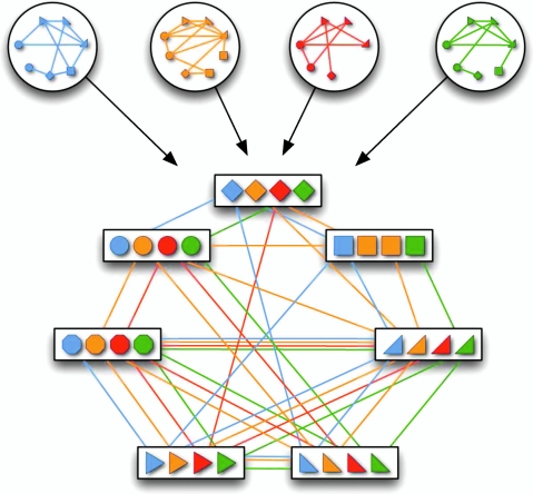
A multiple network alignment is an equivalence relation a over the nodes . An equivalence relation is transitive and partitions V into a set of disjoint equivalence classes (Flannick et al., 2006). A local alignment is a relation over a subset of the nodes in V; a global alignment (Singh et al., 2007) is a relation over all nodes in V. Figure 1 shows an example of an alignment of four protein interaction networks.

FIG. 1.

A network alignment is an equivalence relation. In this example, four protein interaction networks are inputs to multiple network alignment. A network alignment partitions proteins into equivalence classes (indicated by boxes).

Network alignments have a biological interpretation (Flannick et al., 2006). Nodes in the same equivalence class are functionally orthologous (Remm et al., 2001). The subset of nodes in a local alignment represents a conserved module (Hartwell et al., 1999) or pathway.

A scoring function for network alignment is a map , where is the set of potential network alignments of . The global network alignment problem is to find the highest-scoring global network alignment. The traditional local network alignment problem is to find a set of maximally scoring local network alignments. We define a different local network alignment problem: to find the highest-scoring overall set of local network alignments.

2.2. Outline of approach

Græmlin 2.0 searches for local alignments of the input networks in three stages:

Stage 1: Global alignment

Græmlin 2.0 globally aligns the networks—this groups nodes into equivalence classes. The global alignment scoring function computes evolutionary events and is trained on a set of known global network alignments.

Stage 2: Disjoint local alignment

Græmlin 2.0 segments the global alignment into a set of disjoint local alignments—this groups equivalence classes into local alignments. The local alignment scoring function measures local alignment connectivity and is trained on a set of known local network alignments.

Stage 3: Probabilistic assignment

Græmlin 2.0 assigns each node a probabilistic membership in each local alignment—this allows equivalence classes to belong to multiple local alignments. Græmlin 2.0 casts this stage as a supervised learning problem and uses a non-parametric Bayesian classifier.

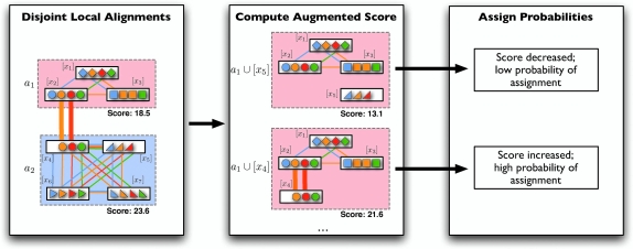
Græmlin 2.0's approach, illustrated in Figure 2, addresses several weaknesses of current local alignment algorithms. First, Græmlin 2.0 performs each alignment stage separately; each stage is simpler to solve than the entire local alignment problem at once.

FIG. 2.

Græmlin 2.0 performs local network alignment in three stages. In stage 1, Græmlin 2.0 globally aligns the input set of networks. In stage 2, it segments the global alignment into a set of disjoint local alignments. In stage 3, it assigns each node a probabilistic membership in each local alignment. Græmlin 2.0 learns scoring functions for the global alignment phase and the disjoint local alignment phase from a training set of known alignments.

Second, Græmlin 2.0 uses feature-based scoring functions that can use arbitrary features of a network alignment. The global alignment scoring function computes evolutionary features that apply to multiple alignment as well as pairwise alignment.

Third, and finally, Græmlin 2.0 learns parameters for its scoring functions from a set of known network alignments. These parameters produce more accurate alignments than manually tuned scoring functions common in current algorithms. Græmlin 2.0 can automatically learn parameters to align any set of networks when given a suitable training set.

Because it searches for alignments in three separate stages, Græmlin 2.0 assumes that it can group nodes into equivalence classes without regard to how it later groups the equivalence classes into local alignments. Græmlin 2.0 therefore assigns two scores to each local alignment: the sum of equivalence class scores determined in the global alignment stage, which measures conservation, and the local alignment score determined in the local alignment stage, which measures connectivity of the nodes in the local alignment. Existing local alignment algorithms produce only one score for each local alignment, which cannot distinguish highly conserved alignments from highly connected alignments.

2.3. Stage 1: Global alignment

The input to the global alignment stage is d networks. The output is a global alignment , where is the set of potential global alignments of the networks and s_g is a scoring function for global network alignment. The global alignment stage therefore groups nodes into equivalence classes.

Græmlin 2.0 hypothesizes that a node will not align to different nodes in different local alignments. It can therefore determine the grouping of nodes into equivalence classes (Stage 1) before it determines the grouping of equivalence classes into local alignments (Stage 2).

2.3.1. Scoring function

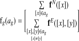
The global alignment scoring function computes “features” (Do et al., 2006a,b) of a global network alignment. Formally, we define a vector-valued global alignment feature function , which maps a global alignment to a numerical feature vector. More specifically, we define a node feature function f^N that maps equivalence classes to a feature vector and an edge feature function f^E that maps pairs of equivalence classes to a feature vector. We then define

(1)

with the first sum over all equivalence classes in the alignment a_g and the second sum over all pairs of equivalence classes in a_g.

Given a numerical parameter vector w_g, the score of a global alignment a_g is s_g(a_g) = w_g · f_g (a_g). The global alignment parameter learning problem is to find w_g. We discuss Græmlin 2.0's parameter learning algorithm below.

The feature function isolates the biological meaning of network alignment. Græmlin 2.0's learning and alignment algorithms make no further biological assumptions. Furthermore, one can define a feature function for any kind of network. Græmlin 2.0's scoring function therefore applies to any set of networks, regardless of the meaning of nodes and edges.

Implementation for protein interaction networks

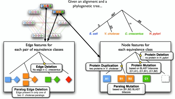
Græmlin 2.0 uses a global alignment feature function that computes evolutionary events. We first describe the feature function for the special case of pairwise global network alignment (the alignment of two networks), and we then generalize the feature function to multiple global network alignment. Figure 3 illustrates the evolutionary events that the feature function computes.

FIG. 3.

Græmlin 2.0's global alignment feature function computes evolutionary events. This figure shows the set of evolutionary events that the node and edge feature functions compute. Græmlin 2.0 uses a phylogenetic tree with branch lengths to determine the events. It first constructs species weight vectors at each internal node of the tree; the weight vector represents the similarity of each extant species to the internal node. It then uses these weight vectors to compute the likely evolutionary events (shown as black boxes) that occur; the Appendix gives precise definitions of these events. Græmlin 2.0 combines the values of the events into a feature vector, and the score of the global alignment is the dot product of a numeric weight vector with the feature vector.

The pairwise node feature function computes the occurrence of four evolutionary events between the species in an equivalence class:

1. Protein deletion: the loss of a protein in one of the two species

2. Protein duplication: the duplication of a protein in one of the two species

3. Protein mutation: the divergence in sequence of two proteins in different species

4. Paralog mutation: the divergence in sequence of two proteins in the same species

The pairwise edge feature function computes the occurrence of two evolutionary events between the species in a pair of equivalence classes:

1. Edge deletion: the loss of an interaction between two pairs of proteins in different species

2. Paralog edge deletion: the loss of an interaction between two pairs of proteins in the same species

The value of each event is one if the event occurs and zero if it does not. The entries in the feature vector are the values of the events.

We take two steps to generalize these pairwise feature functions to multiple network alignment. First, we use a phylogenetic tree to relate species and then sum pairwise feature functions over pairs of species adjacent in the tree, including ancestral species. Second, we modify the feature functions to include evolutionary distance.

These pairwise feature functions generalize to ancestral species pairs. Græmlin 2.0 first computes species weight vectors (Felsenstein, 1973) for each ancestral species. Each species weight vector contains numerical weights that represent the similarity of each extant species to the ancestral species. Græmlin 2.0 uses these species weight vectors, together with the proteins in the equivalence class, to approximate the ancestral proteins in the equivalence class. It then computes pairwise feature functions between the approximate ancestral proteins. The Appendix describes the exact procedure.

In addition, the pairwise feature functions generalize to include evolutionary distance. We augment the feature function by introducing a new feature , where b is the distance between the species pair, for each original feature f_i. Effectively, this transformation allows features to have linear dependencies on b. Additional terms such as have more complex dependencies on b.

The Appendix contains precise definitions of Græmlin 2.0's global alignment feature function as well as precise definitions of all evolutionary events.

2.3.2. Parameter learning algorithm

Inputs

Græmlin 2.0's algorithm to find w_g requires a training set of known global alignments. The training set is a collection of m training examples; each training example specifies a set of networks and their correct alignment .

The parameter learning algorithm requires a loss function . By definition, must be 0 when and positive when (Ratliff et al., 2007). Intuitively, measures the distance of an alignment a_g from the training alignment ; the learned parameter vector should therefore assign higher scores to alignments with smaller loss function values.

To train parameters for the global alignment feature function, we used a training set of KEGG Ortholog (KO) groups (Kanehisa and Goto, 2000). Each training example contained the networks from a set of species, with nodes removed that did not have a KO group. The correct global alignment contained an equivalence class for each KO group.

We also defined a loss function that grows as alignments diverge from the correct alignment . More specifically, let denote the equivalence class of denote the equivalence class of x in a_g. We define , where A \ B denotes the set difference between A and B. This loss function is proportional to the number of nodes aligned in a_g that are not aligned in the correct alignment .

We experimented with the natural opposite of this loss function—the number of nodes aligned in the correct global alignment that are not aligned in a_g. As expected, this alternate loss function resulted in a scoring function that aligned more nodes. We found empirically, however, that the original loss function was more accurate.

Theory

We pose parameter learning as a maximum margin structured learning problem. We find a parameter vector that solves the following convex program (Ratliff et al., 2007):

The constraints in this convex program encourage the learned w_g to satisfy a set of conditions: each training alignment should score higher than all other global alignments a_g by at least . The slack variables ξ_i are penalties for each unsatisfied condition. The objective function is the sum of the penalties with a regularization term that prevents overfitting. Given the low risk of overfitting the few free parameters in our model, we set λ = 0 for convenience. In more complex models with richer feature sets, overfitting can be substantially more severe when the amount of training data is limited; employing effective regularization techniques in such cases is a topic for future research.

We can show (Ratliff et al., 2007) that this constrained convex program is equivalent to the unconstrained minimization problem

(2)

where .

This objective function is convex but nondifferentiable (Ratliff et al., 2007). We can therefore minimize it with subgradient descent (Shor et al., 1985), an extension of gradient descent to nondifferentiable objective functions.

A subgradient of equation (2) is as follows (Ratliff et al., 2007):

where is the optimal global alignment, determined by the loss function and current w_g, of G⁽ⁱ⁾.

Algorithm

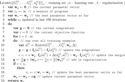
Based on these ideas, the parameter learning algorithm performs subgradient descent. It starts with w_g = 0. Then, it iteratively computes the subgradient g of equation (2) at the current parameter vector w_g and updates w_g ← w_g −αg, where α is the learning rate. The algorithm stops when it performs 100 iterations that do not reduce the objective function. We set the learning rate to a small constant (α = 0.05).

The algorithm for finding is the global alignment inference algorithm. It is a global alignment search algorithm with a scoring function augmented by Δ. Below we present an efficient approximate search algorithm that Græmlin 2.0 uses as an approximate inference algorithm.

The parameter learning algorithm has an intuitive interpretation. At each iteration, it uses the loss function Δ and the current w_g to compute the optimal global alignment. It then decreases the score of features with higher values in the optimal alignment than in the training example and increases the score of features with lower values in the optimal alignment than in the training example. Figure 4 shows the parameter learning algorithm.

FIG. 4.

Græmlin 2.0's parameter learning algorithm.

This parameter learning algorithm has performance guarantees. If the inference algorithm is exact, and if the learning rate is constant, the learning algorithm converges at a linear rate to a small region surrounding the optimal w_g (Nedic and Bertsekas, 2000; Ratliff et al., 2007). A bound on convergence with an approximate inference algorithm is a topic for further research.

2.4. Global alignment search algorithm

Græmlin 2.0's global alignment search algorithm produces a global alignment a_g of a set of input networks. Its goal is to maximize s_g(a_g).

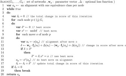
The search algorithm (Fig. 5) serves two roles. It finds the highest scoring global alignment given an optimal learned parameter vector, and it performs inference as part of the parameter learning algorithm.

FIG. 5.

Græmlin 2.0's global alignment search algorithm.

The search algorithm is a local hillclimbing algorithm (Russell and Norvig, 2003). The algorithm is approximate but efficient in practice. It requires that the global alignment feature function decompose into node and edge feature functions as in equation (1).

The search algorithm iteratively performs updates of a current alignment. The initial alignment contains every node in a separate equivalence class. The algorithm then proceeds in a series of iterations. During each iteration, it processes each node and evaluates a series of moves for each node:

• Maintain the node in its current equivalence class.

• Create a new equivalence class with only the node.

• Move the node to another equivalence class.

• Merge the entire equivalence class of the node with another equivalence class.

For each move, Græmlin 2.0 computes the alignment score before and after the move and performs the move that increases the score the most. Once it has processed each node, the algorithm begins a new iteration. It stops when an iteration does not increase the alignment score.

The global alignment search algorithm also performs inference for the parameter learning algorithm. It can use any scoring function that decomposes as in equation (1). Therefore, to perform inference, we need only augment the scoring function with a loss function Δ that also decomposes into node and edge feature functions. The loss function presented above has this property.

The performance of the search algorithm depends on the set of candidate equivalence classes to which processed nodes can move. As a heuristic, it considers as candidates only equivalence classes with a node that has homology (BLAST [Altschul et al., 1997] e-value < 10⁻⁵) to the processed node.

The performance of the search algorithm also depends on the order in which it processes nodes. As a heuristic, it uses node scores—the scoring function with the edge feature function set to zero—to order nodes. For each node, Græmlin 2.0 computes the node score change when it moves the node to each candidate equivalence class. It saves the maximum node score change for each node and then considers nodes in order of decreasing maximum node score change.

In practice, the global alignment search algorithm runs in linear time. To align networks with n total nodes and m total edges, it performs b₁ iterations that each process n nodes. For each node, Græmlin 2.0 computes the change in score when it moves the node to, on average, C candidate classes. Because the global alignment feature function decomposes as in equation (1), to perform each score computation Græmlin 2.0 needs only to examine the candidate class, the node's old class, and the two classes' neighbors. The running time of the search algorithm is therefore O(b₁C(n + m)). Empirically, b₁ is usually a small constant (less than 10). While C can be large, the algorithm runs faster if it only considers candidate classes with high homology to the processed node (BLAST e-value ≪ 10⁻⁵.)

2.5. Stage 2: Disjoint local alignment

The input to Græmlin 2.0's disjoint local alignment stage is a global alignment . The output is a set of disjoint local alignments ; here, is the set of possible partitions of 's equivalence classes into disjoint local alignments, and S_ℓ is a scoring function for a set of local alignments. To allow for nodes that do not belong to any local alignments, Græmlin 2.0 allows local alignments to consist of only one equivalence class. The disjoint local alignment stage therefore groups equivalence classes, which are determined in the global alignment stage, into local alignments.

Græmlin 2.0 searches for the set of local alignments of maximum total score. This search contrasts with the traditional search for a set of maximally scoring alignments, or , where s_ℓ is a scoring function for a single local alignment.

Because it maximizes the total score of all local alignments, Græmlin 2.0 can consider properties of the entire collection of local alignments. For example, it can measure the degree of overlap between local alignments and therefore avoid the heavily overlapping alignments that traditional local aligners produce. In addition, Græmlin 2.0 can add a node to a local alignment even if the node is weakly connected to the local alignment, provided that the node clearly does not belong to any other local alignment.

The disjoint local alignment stage is similar to the traditional clustering problem (Hastie et al., 2001). Græmlin 2.0 can in fact use any clustering algorithm in its disjoint local alignment stage. However, while clustering algorithms can use simple distance metrics for pairwise alignment of networks with single node and edge types, it becomes hard to define robust distance metrics for complex networks with multiple node or edge types (Srinivasan et al., 2007; Kuhn et al., 2007; Sahoo et al., 2007). Below, we present an algorithm that can use arbitrary features of a set of local alignments and generalizes to align complex networks.

2.5.1. Scoring function

Græmlin 2.0's local alignment scoring function uses the same principles as its global alignment scoring function. We therefore outline only the main differences between the global and local alignment scoring functions.

A local alignment feature function f_ℓ maps a local alignment to a numerical feature vector. Given a numerical parameter vector w_ℓ, the score of a local alignment a_ℓ is s_ℓ(a_ℓ) = w_ℓ · f_ℓ(a_ℓ).

The score of a set of local alignments A_ℓ is then , where F_ℓ(A_ℓ) is the sum of the feature vectors of the local alignments in A_ℓ.

Implementation for protein interaction networks

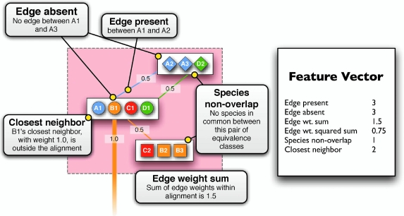
Græmlin 2.0 uses a local alignment feature function that computes the degree of connectivity between equivalence classes in a local alignment. It computes six features, illustrated in Figure 6:

1. Edge present: the number of edges between nodes

2. Edge absent: the number of missing edges between nodes

3. Edge weight sum: the sum of the weights of edges between nodes

4. Edge weight squared sum: the sum of the squared weights of edges between nodes

5. Closest neighbor: the number of nodes in the alignment with a nearest neighbor (the neighbor in the network of maximum edge weight) also in the alignment

6. Species non-overlap: the number of equivalence class pairs that do not have a species in common

FIG. 6.

Græmlin 2.0's local alignment feature function computes features of a local alignment. This figure shows the features that the local alignment feature function computes as well as values of the features for a sample alignment. Græmlin 2.0 combines the values of the features into a feature vector, and the score of the local alignment is the dot product of a numeric weight vector with the feature vector.

These features measure three types of local alignment connectivity. The first four features measure the average edge weight between nodes in the alignment. The fifth feature allows the scoring function to tolerate weakly connected alignments if many nodes are paired with their nearest neighbors. The final feature accounts for equivalence class pairs that the first five features ignore—equivalence class pairs with disjoint sets of species lack the potential to interact and are distinct from pairs that have the potential to interact but do not.

We chose these features after examining local alignments in our training set that existing aligners do not find. We experimented with other features that did not depend on network edges, including the size of the alignment and amount of synteny present in the alignment, but found that the edge-based features played by far the largest role in the scoring function. As networks incorporate multiple data types and become more accurate, other features will likely become more important.

2.5.2. Parameter learning algorithm

The parameter learning algorithm in Figure 4 applies to both the global and local alignment scoring functions. The only differences between the global and local alignment parameter learning algorithms are the form of the training set, the definition of the loss function, and the definition of the inference algorithm.

To train parameters for the local alignment feature function, we used a training set of KEGG pathways. Each training example contained the networks from a set of species and a correct global alignment with an equivalence class for each KO group. The correct set of local alignments contained a local alignment for each KEGG pathway.

In addition, we set the loss function to a constant value. We experimented with a loss function analogous to that used in the global alignment parameter learning algorithm, but we found such a loss function computationally prohibitive.

The local alignment inference algorithm is a local alignment search algorithm with a scoring function augmented by the loss function. Below we present an approximate local alignment search algorithm that Græmlin 2.0 uses as an approximate inference algorithm.

2.5.3. Disjoint local alignment search algorithm

Græmlin 2.0's disjoint local alignment search algorithm segments the equivalence classes in a global alignment a_g into a disjoint set of local alignments A_ℓ. Its goal is to maximize the total score S_ℓ(A_ℓ).

As it does for global alignment, Græmlin 2.0 uses a local hillclimbing method for disjoint local alignment. The algorithm begins with an initial set of alignments in which every equivalence class is in a separate local alignment. Then, it performs a series of iterations, each of which processes each equivalence class in turn. Græmlin 2.0 computes the change in score resulting from moving the equivalence class to any other local alignment, and performs the move that increases the score the most. It stops when it performs a iteration that does not increase the score.

In practice, the local alignment search algorithm runs in linear time. To segment a global alignment of networks with n total nodes and m total edges, it performs b₂ iterations, each of which processes at most n equivalence classes. With suitable caching (technical details omitted), Græmlin 2.0 must only examine the edges incident to an equivalence class to compute the change in score resulting from moving the equivalence class to each alignment. The total running time of the algorithm is therefore O(b₂ × (n + m)); because b₂ is usually a small constant (less than 10), it is efficient in practice.

The local alignment algorithm is relatively simple compared to other existing local alignment algorithms. However, we show in the Results (Section 3) that Græmlin 2.0 produces accurate local alignments, mainly because it uses an accurate scoring function.

2.6. Stage 3: Probabilistic assignment

The input to Græmlin 2.0's probabilistic assignment stage is a set of disjoint local alignments . The output, for each local alignment a_ℓ and each equivalence class [x] in the global alignment, is the probability that [x] belongs to a_ℓ.

Græmlin 2.0 uses these probabilities to obtain the final set of local alignments. To each local alignment a_ℓ in , it adds all equivalence classes that belong a_ℓ with probability greater than a user-specified threshold. Lower thresholds yield larger but less accurate local alignments.

Græmlin 2.0 uses a supervised learning algorithm to compute probabilities, with the set of disjoint local alignments as a training set. It bases the probability that an equivalence class [x] belongs to a local alignment a_ℓ on , the difference between the score of a_ℓ with [x] and the score of a_ℓ without [x]. Figure 7 illustrates the idea.

FIG. 7.

Græmlin 2.0 assigns probabilistic membership in local alignments. For each equivalence class [x] and each local alignment a_ℓ, Græmlin 2.0 computes the change in score that results when it adds [x] to a_ℓ. Intuitively, the probability that [x] belongs to a_ℓ is high if the change in score when Græmlin 2.0 adds [x] to a_ℓ is high relative to the change in score when it adds other nodes to a_ℓ.

In detail, the algorithm first builds a separate Bayesian classifier for each disjoint local alignment. It computes three statistics for each equivalence class [x] and each local alignment a_ℓ:

• Pr([x]∈a_ℓ), the prior probability that [x] is in a_ℓ

• , the conditional distribution of given that [x] is in a_ℓ

• , the conditional distribution of given that [x] is not in a_ℓ

The algorithm then uses Bayes's rule to assign [x] to a_ℓ with probability

(3)

where

Græmlin 2.0 estimates Pr([x]∈a_ℓ) as the ratio of the number of equivalence classes in a_ℓ to the total number of equivalence classes in all local alignments.

Græmlin 2.0 estimates the two conditional distributions using kernel density estimation (Duda et al., 2000). For samples from , it uses the values for the equivalence classes already in a_ℓ. For samples from , it uses the values for the equivalence classes not already in a_ℓ. For each estimation, it uses a Gaussian kernel, with bandwidth chosen by Silverman's “rule of thumb” (Silverman, 1986).

3. Results

3.1. Accuracy benchmarks

We performed two sets of benchmarks. The first measured the accuracy of the equivalence class groupings found in the global alignment stage. The second measured the overall accuracy of Græmlin 2.0's local alignments.

3.1.1. Equivalence class accuracy comparisons

Experimental setup

We tested equivalence class accuracy on three different network datasets: IntAct (Kerrien et al., 2007), DIP (Xenarios et al., 2002), and the Stanford Network Database (Srinivasan et al., 2006) (SNDB). We ran pairwise alignments of the human and mouse IntAct networks, yeast and fly DIP networks, Escherichia coli K12 and Salmonella typhimurium LT2 SNDB networks, and E. coli and Caulobacter crescentus SNDB networks. We also ran a three-way alignment of the yeast, worm, and fly DIP networks, and a six-way alignment of E. coli, S. typhimurium, Vibrio cholerae, Campylobacter jejuni NCTC 11168, Helicobacter pylori 26695, and C. crescentus SNDB networks.

We used KO groups (Kanehisa and Goto, 2000) for our equivalence class comparison metrics. To compute each metric, we first removed all nodes in the alignment without a KO group, and we then removed all equivalence classes with only one node. We then defined an equivalence class as correct if every node in it had the same KO group.

To measure specificity, we computed two metrics:

1. the fraction of equivalence classes that were correct (C_eq)

2. the fraction of nodes that were in correct equivalence classes (C_node)

To measure sensitivity, we computed two metrics:

1. the total number of nodes that were in correct equivalence classes (Cor)

2. the total number of equivalence classes that contained k species, for

We used cross-validation to test Græmlin 2.0. For each set of networks, we partitioned the KO groups into ten equal sized test sets. For each test set, we trained Græmlin 2.0 on the KO groups not in the test set as described in the Methods section. We then aligned the networks and computed our metrics on only the KO groups in the test set. Our final numbers for a set of networks were the average of our metrics over the ten test sets.

To limit biases from the averaging process we used cross validation to test all aligners. For aligners other than Græmlin 2.0, we aligned the networks only one time. However, we did not compute our metrics on all KO groups at once; instead, we computed our metrics separately for each test set and then averaged the numbers.

As a final check that our test and training sets were independent, we computed similar metrics using Gene Ontology (GO) categories (Ashburner et al., 2000; Sharan et al., 2005b) instead of KO groups. We do not report the results of these tests because they are similar to the results of our tests on KO groups.

We compared Græmlin 2.0 to the local aligners NetworkBLAST (Sharan et al., 2005b), MaWISh (Koyuturk et al., 2006), and Græmlin (Flannick et al., 2006), as well as the global aligner IsoRank (Singh et al., 2007) and a global aligner (Græmlin-global) that used Græmlin 2.0's global alignment search algorithm with Græmlin's scoring function.

While we simultaneously compared Græmlin 2.0 to IsoRank and Græmlin-global, we compared Græmlin 2.0 to each local aligner separately. According to our definitions, local aligners may have lower sensitivity than global aligners simply because local aligners only align nodes that belong to conserved modules while global aligners align all nodes. Therefore, for each comparison to a local aligner, we removed all equivalence classes in Græmlin 2.0's output that did not contain a node in the local aligner's output.

Performance comparisons

Table 1 shows that, with respect to the alignment of proteins, Græmlin 2.0 is the most specific aligner. Across all datasets, it produces both the highest fraction of correct equivalence classes as well as the highest fraction of nodes in correct equivalence classes.

Table 1.

Græmlin 2.0 Aligns Nodes with Higher Specificity

	Average equivalence class consistency
	SNDB						IntAct		DIP
	eco/stm		eco/cce		6-way		hsa/mmu		sce/dme		3-way
	Ceq	Cnode	Ceq	Cnode	Ceq	Cnode	Ceq	Cnode	Ceq	Cnode	Ceq	Cnode
Local aligner comparisons
NB	0.77	0.45	0.78	0.50	—	—	0.33	0.06	0.39	0.14	—	—
Gr2.0	0.95	0.94	0.79	0.78	—	—	0.83	0.81	0.58	0.58	—	—
MW	0.84	0.64	0.77	0.54	—	—	0.59	0.36	0.45	0.37	—	—
Gr2.0	0.97	0.96	0.77	0.76	—	—	0.88	0.86	0.90	0.91	—	—
Gr	0.80	0.77	0.69	0.64	0.76	0.67	0.59	0.53	0.33	0.29	0.23	0.15
Gr2.0	0.96	0.95	0.82	0.81	0.86	0.85	0.86	0.84	0.61	0.61	0.57	0.57
Global aligner comparisons
GrG	0.86	0.86	0.72	0.72	0.80	0.81	0.64	0.64	0.68	0.68	0.71	0.71
Iso	0.91	0.91	0.65	0.65	—	—	0.62	0.62	0.63	0.63	—	—
Gr2.0	0.96	0.96	0.78	0.78	0.87	0.87	0.81	0.80	0.73	0.73	0.76	0.76

We measured the fraction of correct equivalence classes (C_eq) and the fraction of nodes in correct equivalence classes (C_node), as described in the text. We compared Græmlin 2.0 (Gr2.0) to NetworkBLAST (NB), MaWISh (MW), Græmlin (Gr), IsoRank (Iso), and a global aligner that used Græmlin 2.0's alignment search algorithm with Græmlin's scoring function (GrG). As described in the text, we ran four pairwise alignments, a three-way alignment, and a six-way alignment. For each comparison between Græmlin 2.0 and a local aligner, we removed equivalence classes from Græmlin 2.0's output that did not contain a node in the local aligner's output; Table 2 shows the number of remaining nodes for each aligner. MaWISh and IsoRank are not multiple aligners; NetworkBLAST can align only up to three species and aborted on the three-way alignment.

eco, E. coli; stm, S. typhimurium; cce, C. crescentus; hsa, human; mmu, mouse; sce, yeast; dme, fly.

Table 2 shows that, with respect to the alignment of proteins, Græmlin 2.0 is also the most sensitive aligner. In the SNDB pairwise alignments, Græmlin 2.0 and IsoRank produce the most number of nodes in correct equivalence classes. In the other tests, Græmlin 2.0 produces the most number of nodes in correct equivalence classes.

Table 2.

Græmlin 2.0 Aligns Nodes with Higher Sensitivity

	Number of nodes in correct equivalence classes
	SNDB						IntAct		DIP
	eco/stm		eco/cce		6-way		hsa/mmu		sce/dme		3- way
	Cor	Tot	Cor	Tot	Cor	Tot	Cor	Tot	Cor	Tot	Cor	Tot
Local aligner comparisons
NB	457	1016	346	697	—	—	65	1010	43	306	—	—
Gr2.0	627		447		—		258		155		—
MW	1309	2050	458	841	—	—	87	241	10	27	—	—
Gr2.0	1611		553		—		181		20		—
Gr	985	1286	546	847	1524	2287	108	203	35	122	27	180
Gr2.0	1157		608		2216		151		75		86
Global aligner comparisons
GrG	1496		720		2388		268		384		546
Iso	2026	—	1014	—	—	—	306	—	534	—	—	—
Gr2.0	2024		1012		3578		350		637		827

We measured the number of nodes in correct equivalence classes (Cor), as described in the text. To show the number of nodes considered in each local aligner comparison, we also measured the number of nodes aligned by each local aligner (Tot). Methodology and abbreviations are the same as in Table 1.

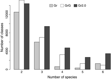
Figure 8 shows that Græmlin 2.0 also finds more cross-species conservation than Græmlin and Græmlin-global. Relative to Græmlin and Græmlin-global, Græmlin 2.0 produces two to five times as many equivalence classes with four, five, and six species.

FIG. 8.

Græmlin 2.0 finds more cross-species conservation. We counted the number of equivalence classes that contained k species for k = 2, 3, 4, 5, 6 as described in the text. We compared Græmlin 2.0 (Gr2.0) to Græmlin (Gr) and a global aligner (GrG) that used Græmlin 2.0's alignment search algorithm with Græmlin's scoring function. We ran the six-way alignment described in the text.

We performed our tests on a 2.2-GHz machine with 4 GB of RAM. For each pairwise alignment, Græmlin 2.0, MaWISh, Græmlin, and Græmlin-global ran in less than a minute, while IsoRank and NetworkBLAST each ran for over an hour. For each pairwise alignment training run, Græmlin 2.0 ran for under 10 minutes. On the six-way alignment, Græmlin 2.0, Græmlin, and Græmlin-global each ran for under 3 minutes, and Græmlin 2.0 trained in under 45 minutes.

3.1.2. Local alignment accuracy comparisons

Experimental setup

We tested local alignment accuracy on DIP and SNDB (the IntAct networks produced local alignments too small for meaningful comparisons). We ran pairwise alignments of the yeast and fly DIP networks and the E. coli and C. crescentus SNDB networks, and we ran a six-way alignment of the E. coli, S. typhimurium, V. cholerae, C. jejuni, H. pylori, and C. crescentus SNDB networks.

We used KEGG pathways (Kanehisa and Goto, 2000) for our local alignment comparison metrics. To compute each metric, we first removed all nodes in the alignment not assigned to a KEGG pathway, and we then removed all local alignments with only one equivalence class. For each local alignment, we defined the closest KEGG as the KEGG pathway that overlapped the local alignment the most. For each KEGG pathway, we defined the closest alignment as the local alignment that overlapped the KEGG pathway the most.

To measure specificity and sensitivity, we computed two metrics:

1. the average, over all local alignments, of the fraction of nodes in the alignment that were also in the closest KEGG (Spec)

2. the average, over all KEGG pathways, of the fraction of nodes in the KEGG pathway that were also in the closest alignment (Sens)

Intuitively, the closest KEGG and closest alignment concepts attempt to find the best match between KEGG pathways and local alignments. Our specificity metric (Spec) measures the degree to which each local alignment contains only nodes that belong to a single KEGG pathway, and our sensitivity metric (Sens) measures the degree to which each KEGG pathway appears in a single local alignment.

We also computed benchmarks for local alignment accuracy used in the past (Flannick et al., 2006), which count the number of KEGG pathways overlapped by a local alignment. However, Græmlin 2.0 by nature will produce alignments that overlap more KEGG pathways because it includes every node in its set of local alignments while the other local aligners include only some nodes in their sets of local alignments. We found that our sensitivity metric was less biased in favor of Græmlin 2.0.

As we did with the tests of equivalence class accuracy, we used cross-validation to test Græmlin 2.0. For each set of networks, we partitioned the KEGG pathways into ten equal sized test sets. For each test set, we trained Græmlin 2.0 on the KEGG pathways not in the test set. We then aligned the networks and computed our metrics on only the KEGG pathways groups in the test set. Our final numbers for a set of networks were the average of our metrics over the ten test sets. We applied this procedure to all tested aligners to limit biases arising from the averaging process.

We also ran tests using various levels of the GO hierarchy in place of KEGG pathways. We omit the results for brevity, because they were very similar to those we obtained with KEGG pathways.

We compared Græmlin 2.0 to NetworkBLAST (Sharan et al., 2005b), MaWISh (Koyuturk et al., 2006), and Græmlin (Flannick et al., 2006). We used a threshold of 0.9 to obtain Græmlin 2.0's final set of local alignments from the results of its probabilistic assignment stage. Lower thresholds yielded a sensitivity/specificity trade-off as expected, but we found the loss in specificity to outweigh the increase in sensitivity.

Performance comparisons

Table 3 shows that, with respect to the grouping of proteins into modules, Græmlin 2.0 is significantly more sensitive than existing aligners and still maintains high specificity. Græmlin 2.0's sensitivity increase is due in part to its ability to find weakly conserved and sparsely connected modules, two of which we discuss below.

Table 3.

Græmlin 2.0 Groups Nodes into Modules with Higher Accuracy

Accuracy of local alignments
	SNDB				DIP
	eco/cce		6-way		sce/dme
	Sens	Spec	Sens	Spec	Sens	Spec
NetworkBLAST	0.33	0.64	—	—	0.14	0.52
Ma WISh	0.22	0.80	—	—	0.12	0.71
Græmlin	0.26	0.79	0.17	0.73	0.13	0.65
Græmlin 2.0	0.33	0.78	0.32	0.71	0.21	0.72

As described in the text, we measured the sensitivity (Sens) and specificity (Spec) of local alignments produced by Græmlin 2.0, NetworkBLAST, MaWISh, and Græmlin on the DIP and the Stanford Network Database network datasets. Abbreviations are the same as in Table 1.

All local aligners ran in under 10 minutes, except for NetworkBLAST, which ran in a few hours. Training runs for Græmlin 2.0 took less than 5 hours, although parameters nearly reached their final values within the first hour.

3.2. Sample alignments

In this section, we give examples of conserved modules that Græmlin 2.0 finds but existing aligners miss. We focus on these weakly conserved modules to illustrate Græmlin 2.0's performance advantages; all aligners find highly conserved modules. In addition, we give examples of the multiple alignment memberships that Græmlin 2.0's probabilistic assignment stage produces.

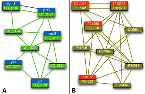
Figure 9A shows an alignment of part of the module for glutathione metabolism in E. coli and C. crescentus. The alignment is weakly connected and edges are weakly conserved, which causes aligners like MaWISh and Græmlin that search for only very highly conserved protein complexes to miss it. Græmlin 2.0 finds this module because it learns from examples in its training set that many modules are weakly conserved and weakly connected. Furthermore, because it searches for the entire set of local alignments at once, Græmlin 2.0 adds the weakly connected nodes to the alignment when it determines that they belong to no other high scoring alignments.

FIG. 9.

Græmlin 2.0 finds more complete functional modules. This figure shows two local alignments that Græmlin 2.0 finds. Græmlin 2.0 is more sensitive than existing network aligners, in part because it learns parameters on a training set with weakly conserved and sparsely connected modules. (A) Græmlin 2.0 tolerates weak connectivity in a local alignment of nodes involved in glutathione metabolism (blue, E. coli; green, C. crescentus). (B) Græmlin 2.0 finds a weakly conserved but highly connected local alignment of part of the RNA polymerase complex (red, yeast; gold, fly).

Figure 9B shows an alignment of a portion of RNA polymerase in yeast and fly. While the module has stronger connectivity than that in Figure 9A, edge conservation is still weak, with edges present predominantly in yeast and all but absent in fly. In addition, several fly nodes are missing from the alignment (orthologs of P34087 and P41896) or from the network entirely (orthologs of Q06834, P27999, and P20434). Græmlin 2.0 recognizes the alignment as weakly conserved but highly connected because it uses separate scoring functions for global and local alignment.

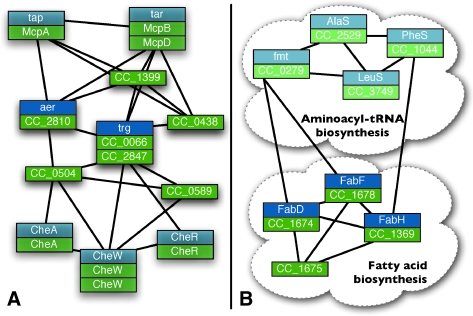
Græmlin 2.0's probabilistic assignment algorithm reveals additional members of conserved modules and also finds clear connections between separate modules. Figure 10A shows an alignment of part of the chemotaxis module in C. crescentus and E. coli. In the set of disjoint alignments, half of the module is included in an alignment of the flagellum module instead. When Græmlin 2.0 assigns each node multiple probabilistic memberships, it places the remaining chemotaxis nodes into the alignment of the chemotaxis module. However, the chemotaxis nodes originally included in the flagellum alignment receive a relatively low probability of membership in the chemotaxis alignment, indicating their relatively strong connection to the flagellum module.

FIG. 10.

Probabilistic assignment expands and clarifies functional modules. This figures shows two alignments augmented by Græmlin 2.0's probabilistic assignment. Nodes with lower membership probabilities are shaded with fainter colors; black lines show the presence of one or more edges between a pair of equivalence classes. (A) Græmlin 2.0 identifies proteins in the chemotaxis module, but which are more strongly connected to the flagellum module, as members of both modules during the probabilistic assignment stage. (B) Græmlin 2.0 identifies two connected but distinct pathways for aminoacyl-tRNA biosynthesis and fatty acid biosynthesis during the probabilistic assignment stage.

Figure 10B shows parts of the modules for aminoacyl-tRNA biosynthesis and fatty acid biosynthesis. In the original set of disjoint alignments, Græmlin 2.0 places nodes from the two modules into separate alignments. However, the probabilistic assignment stage combines the two modules into one alignment. The nodes in the aminoacyl-tRNA biosynthesis module have a relatively low probability of membership in the fatty acid biosynthesis alignment, which indicates that the modules are distinct.

4. Discussion

In this article, we presented Græmlin 2.0, a multiple network aligner with a multi-stage approach to local network alignment, new feature-based scoring functions for global and local network alignment, an algorithm that automatically learns parameters for the scoring functions, and algorithms that use the scoring functions to approximately align multiple networks in linear time. We implemented Græmlin 2.0 for protein interaction network alignment and showed that it has higher accuracy than existing network alignment algorithms across multiple network datasets.

Græmlin 2.0 allows users to easily apply network alignment to their network dataset. Its learning algorithm automatically learns parameters specific to any set of networks. In contrast, existing alignment algorithms require manual recalibration to adjust parameters to different datasets.

In particular, Græmlin 2.0 can in principle learn parameters that account for noisy networks. More false positive or false negative interactions in a network will lead to a training set with fewer conserved edges and fewer edges between functionally linked proteins. In such networks, Græmlin 2.0 will learn lower weights for its edge features relative to its node features. For example, as expected in light of recent doubts about the accuracy of literature-curated and experimentally derived networks (Srinivasan et al., 2006; Cusick et al., 2009), Græmlin 2.0 assigns a relatively low weight to the edge deletion feature when trained on networks in DIP and IntAct. In contrast, it assigns a higher weight to the edge deletion feature when trained on networks in the Stanford Network Database, which past studies have shown to more accurately recapitulate known functional linkages (Srinivasan et al., 2006). A complete study of the performance of Græmlin 2.0 on networks with different noise levels, as well as the inclusion into its feature function of features that more explicitly measure network noise, is a topic for further research.

Græmlin 2.0 also extends in principle beyond protein interaction network alignment. As more experimental data gathers and network integration algorithms improve, network datasets with multiple data types will appear (Srinivasan et al., 2007), such as networks with interactions between proteins and DNA (Zhang et al., 2005; Tan et al., 2007), networks with physical as well as genetic interactions (Kelley and Ideker, 2005; Ulitsky et al., 2008), expression networks with boolean edges (Sahoo et al., 2007), and metabolic networks with chemical compounds (Kuhn et al., 2007). With future work to redefine Græmlin 2.0's feature functions, its scoring function and parameter learning algorithm will apply to these kinds of networks.

Several future research directions might further improve the performance of Græmlin 2.0. While its scoring function for global alignment models node and edge evolution (Flannick et al., 2008), its scoring function for disjoint local alignment does not model module evolution. Features such as module “cohesion” (Campillos et al., 2006) may improve the local alignment scoring function. In addition, future work might combine the ideas behind some of the more sophisticated search algorithms proposed recently (Singh et al., 2007; Zhenping et al., 2007) with Græmlin 2.0's accurate scoring function.

5. Appendix

A. Global alignment feature function definition

This section presents precise definitions of Græmlin 2.0's global alignment feature function and the evolutionary events that the feature function computes. The feature function for local alignment uses the same principles.

We define evolutionary events for possibly ancestral species. We assume that we have n extant species and m ancestral species ,¹ all related by a phylogenetic tree.

Each species i∈[1: n + m] is represented by a species weight vector represents the similarity of species j∈[1: n] to species i. We can use a phylogenetic tree to compute the weight vectors efficiently (Felsenstein, 1973; Altschul et al., 1989). Each extant species j∈[1: n] has a species weight vector .

We denote an equivalence class [x] as a set of proteins is the projection of [x] to species i.

A.1. Node feature function

We compute the node feature function f^N for an equivalence class [x] as follows. First, we compute events for species r, the species at the phylogenetic tree root.

Protein present

We define as p_i = 1 if and 0 otherwise.

• is the probability that species r has a protein in [x].

• is the probability that species r does not have a protein in [x].

Protein count

We define , as , the number of proteins that species i has in [x].

• is the expected number of proteins species r has in [x], given that r has a protein.

• 

The protein present and protein count features describe the most recent common ancestor of the extant species in the equivalence class. The protein present feature estimates the probability that the ancestor had a protein homologous to those in the equivalence class, and the protein count feature estimates the expected number of ancestral proteins homologous to those in the equivalence class.

Next, we compute events for all pairs of species i, j∈[1: n + m], i ≠ j adjacent in the tree.

Protein deletion

We define p(k) = s^k · p as the probability that species k has a protein in [x].

• is the probability a protein deletion occurs between species i and j.

• is the probability a protein deletion does not occur between species i and j.

Protein duplication

We define as the expected numbers of proteins that species k has in [x].

• is the expected number of proteins gained between species i and j.

If either species i or j have no proteins in [x], then has value 0.

Protein mutation

We define a species pair weight matrix . We define as

where b(p,q) is the BLAST bitscore (Altschul et al., 1997) of proteins p and q. B_kl is the average bitscore among the proteins in species k and l. B_kl equals 0 if either species k or l has no proteins in [x].

• , the sum of entry-wise products, is the expected bitscore between the proteins in species i and j.

• 

• 

• 

Features 1 allow Græmlin 2.0's scoring function to include nonlinear dependencies on the BLAST bitscore of the proteins.

Finally, we compute events for all extant species i ∈ [1 : n].

Paralog mutation

• is the expected average bitscore between a protein in species i and its paralogs.

• 

• 

• 

A.2. Edge feature function

We compute the edge feature function f^E for equivalence classes [x] and [y] as follows. First, we compute events for all pairs of species i, j∈[1: n + m], i ≠ j adjacent in the tree.

Edge deletion

For , we define e(k, p, q) = 1 if there is an edge between p and q and 0 otherwise. We then define as

which represents the average probability that species k has an edge. We define e_k as null if is empty. We define

which represent the probabilities that species i and j have edges.

• is the probability that an edge is lost between species i and j.

• is the probability that an edge is not lost between i and j.

Next, we compute events for all extant species i∈[1 : n].

Paralog edge deletion

We define as

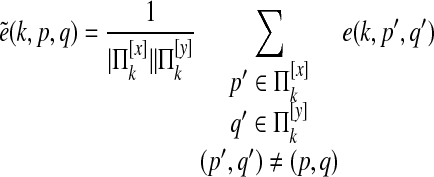which represents the probability, ignoring p and q, that species k has an edge.

• is the average probability an edge is lost between a pair of proteins in species i and all other pairs of proteins in species i.

• is the average probability an edge is not lost between a pair of proteins in species i and all other pairs of proteins in species i.

For pairwise alignment of two species s and t, the final node feature function is

and the final edge feature function is

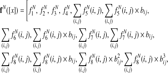
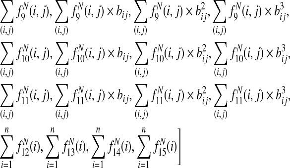
For multiple alignment, the final node feature function is

and the final edge feature function is

where b_ij is the branch length between species i and j, the sums over (i,j) are taken over branches of the phylogenetic tree, and the sums i are taken over the leaves of the tree.

Acknowledgments

J.F. was supported in part by a Stanford Graduate Fellowship. A.N. was supported by the NLM (training grant LM-07033) and the NIH (grant UHG003162). C.B.D. was funded by an NSF Fellowship. B.S.S. was funded by an NSF VIGRE postdoctoral fellowship (NSF grant EMSW21-VIGRE 0502385). This work was supported in part by NSF grant OBI-0640211-001.

Disclosure Statement

No competing financial interests exist.

References

- Altschul S.F. Carroll R.J. Lipman D.J. Weights for data related by a tree. J. Mol. Biol. 1989;207:647–653. doi: 10.1016/0022-2836(89)90234-9. [DOI] [PubMed] [Google Scholar]
- Altschul S.F. Madden T.L. Schaffer A.A., et al. Gapped BLAST and PSI-BLAST: a new generation of protein database search programs. Nucleic Acids Res. 1997;25:3389–3402. doi: 10.1093/nar/25.17.3389. [DOI] [PMC free article] [PubMed] [Google Scholar]
- Ashburner M. Ball C.A. Blake J. A., et al. Gene ontology: tool for the unification of biology. The Gene Ontology Consortium. Nat. Genet. 2000;25:25–29. doi: 10.1038/75556. [DOI] [PMC free article] [PubMed] [Google Scholar]
- Berg J. Lssig M. Local graph alignment and motif search in biological networks. Proc. Natl. Acad. Sci. USA. 2004;101:14689–14694. doi: 10.1073/pnas.0305199101. [DOI] [PMC free article] [PubMed] [Google Scholar]
- Berg J. Lassig M. Cross-species analysis of biological networks by Bayesian alignment. Proc. Natl. Acad. Sci. USA. 2006;103:10967–10972. doi: 10.1073/pnas.0602294103. [DOI] [PMC free article] [PubMed] [Google Scholar]
- Campillos M. von Mering C. Jensen L.J., et al. Identification and analysis of evolutionarily cohesive functional modules in protein networks. Genome Res. 2006;16:374–382. doi: 10.1101/gr.4336406. [DOI] [PMC free article] [PubMed] [Google Scholar]
- Cusick M.E. Klitgord N., et al. Interactome: gateway into systems biology. Hum. Mol. Genet. 2005;14:171–181. doi: 10.1093/hmg/ddi335. [DOI] [PubMed] [Google Scholar]
- Cusick M.E. Yu H. Smolyar A., et al. Literature-curated protein interaction datasets. Nat. Methods. 2009;6:39–46. doi: 10.1038/nmeth.1284. [DOI] [PMC free article] [PubMed] [Google Scholar]
- Do C.B. Gross S.S. Batzoglou S. Contralign: discriminative training for protein sequence alignment. Proc. RECOMB 2006. 2006a:160–174. [Google Scholar]
- Do C.B. Woods D.A. Batzoglou S. CONTRAfold: RNA secondary structure prediction without physics-based models. Bioinformatics. 2006b;22:90–98. doi: 10.1093/bioinformatics/btl246. [DOI] [PubMed] [Google Scholar]
- Dost B. Shlomi T. Ruppin E., et al. Qnet: a tool for querying protein interaction networks. Proc. RECOMB 2007. 2007:1–15. doi: 10.1089/cmb.2007.0172. [DOI] [PubMed] [Google Scholar]
- Duda R.O. Hart P.E. Stork D.G. Pattern Classification. Wiley-Interscience Publication; New York: 2000. [Google Scholar]
- Dutkowski J. Tiuryn J. Identification of functional modules from conserved ancestral protein-protein interactions. Bioinformatics. 2007;23:i149–i158. doi: 10.1093/bioinformatics/btm194. [DOI] [PubMed] [Google Scholar]
- Felsenstein J. Maximum-likelihood estimation of evolutionary trees from continuous characters. Am. J. Hum. Genet. 1973;25:471–492. [PMC free article] [PubMed] [Google Scholar]
- Flannick J. Novak A. Srinivasan B.S., et al. Graemlin: general and robust alignment of multiple large interaction networks. Genome Res. 2006;16:1169–1181. doi: 10.1101/gr.5235706. [DOI] [PMC free article] [PubMed] [Google Scholar]
- Flannick J. Novak A. Do C.B., et al. Automatic parameter learning for multiple network alignment. Proc. RECOMB 2008. 2008:214–231. doi: 10.1089/cmb.2009.0099. [DOI] [PMC free article] [PubMed] [Google Scholar]
- Hartwell L.H. Hopfield J.J. Leibler S., et al. From molecular to modular cell biology. Nature. 1999;402:47–52. doi: 10.1038/35011540. [DOI] [PubMed] [Google Scholar]
- Hastie T. Tibshirani R. Friedman J.H. The Elements of Statistical Learning. Springer; New York: 2001. [Google Scholar]
- Hirsh E. Sharan R. Identification of conserved protein complexes based on a model of protein network evolution. Bioinformatics. 2007;23:170–176. doi: 10.1093/bioinformatics/btl295. [DOI] [PubMed] [Google Scholar]
- Kalaev M. Bafna V. Sharan R. Fast and accurate alignment of multiple protein networks. Proc. RECOMB 2008. 2008:246–256. doi: 10.1089/cmb.2009.0136. [DOI] [PubMed] [Google Scholar]
- Kanehisa M. Goto S. KEGG: Kyoto Encyclopedia of Genes and Genomes. Nucleic Acids Res. 2000;28:27–30. doi: 10.1093/nar/28.1.27. [DOI] [PMC free article] [PubMed] [Google Scholar]
- Kelley R. Ideker T. Systematic interpretation of genetic interactions using protein networks. Nat. Biotechnol. 2005;23:561–566. doi: 10.1038/nbt1096. [DOI] [PMC free article] [PubMed] [Google Scholar]
- Kelley B.P. Sharan R. Karp R.M., et al. Conserved pathways within bacteria and yeast as revealed by global protein network alignment. Proc. Natl. Acad. Sci. USA. 2003;100:11394–11399. doi: 10.1073/pnas.1534710100. [DOI] [PMC free article] [PubMed] [Google Scholar]
- Kerrien S. Alam-Faruque Y. Aranda B., et al. IntAct–open source resource for molecular interaction data. Nucleic Acids Res. 2007;35:561–565. doi: 10.1093/nar/gkl958. [DOI] [PMC free article] [PubMed] [Google Scholar]
- Koyuturk M. Kim Y. Topkara U., et al. Pairwise alignment of protein interaction networks. J. Comput. Biol. 2006;13:182–199. doi: 10.1089/cmb.2006.13.182. [DOI] [PubMed] [Google Scholar]
- Kuhn M. von Mering C. Campillos M., et al. STITCH: interaction networks of chemicals and proteins. Nucleic Acids Res. 2007:D684–688. doi: 10.1093/nar/gkm795. [DOI] [PMC free article] [PubMed] [Google Scholar]
- Nedic A. Bertsekas D. Convergence rate of incremental subgradient algorithms. 2000. www.citeseer.ist.psu.edu/nedic00convergence.html. [Jun 29;2009 ]. www.citeseer.ist.psu.edu/nedic00convergence.html
- Pereira-Leal J.B. Levy E.D. Teichmann S.A. The origins and evolution of functional modules: lessons from protein complexes. Philos. Trans. R. Soc. Lond. B Biol. Sci. 2006;361:507–517. doi: 10.1098/rstb.2005.1807. [DOI] [PMC free article] [PubMed] [Google Scholar]
- Pinter R.Y. Rokhlenko O. Yeger-Lotem E., et al. Alignment of metabolic pathways. Bioinformatics. 2005;21:3401–3408. doi: 10.1093/bioinformatics/bti554. [DOI] [PubMed] [Google Scholar]
- Ratliff N. Bagnell J. Zinkevich M. (Online) subgradient methods for structured prediction. 11th Int. Conf. AIStats..2007. [Google Scholar]
- Remm M. Storm C.E. Sonnhammer E.L. Automatic clustering of orthologs and in-paralogs from pairwise species comparisons. J. Mol. Biol. 2001;314:1041–1052. doi: 10.1006/jmbi.2000.5197. [DOI] [PubMed] [Google Scholar]
- Russell S. Norvig P. Artificial Intelligence: A Modern Approach. 2nd. Prentice-Hall; Englewood Cliffs, NJ: 2003. [Google Scholar]
- Sahoo D. Dill D. Gentles A., et al. Bodean implication networks derived from large-scale, whole genome microarray datasets. Genome Biol. 2008 Oct;9:R157. doi: 10.1186/gb-2008-9-10-r157. [DOI] [PMC free article] [PubMed] [Google Scholar]
- Sharan R. Ideker T. Modeling cellular machinery through biological network comparison. Nat. Biotechnol. 2006;24:427–433. doi: 10.1038/nbt1196. [DOI] [PubMed] [Google Scholar]
- Sharan R. Ideker T. Kelley B., et al. Identification of protein complexes by comparative analysis of yeast and bacterial protein interaction data. J. Comput. Biol. 2005a;12:835–846. doi: 10.1089/cmb.2005.12.835. [DOI] [PubMed] [Google Scholar]
- Sharan R. Suthram S. Kelley R.M., et al. Conserved patterns of protein interaction in multiple species. Proc. Natl. Acad. Sci. USA. 2005b;102:1974–1979. doi: 10.1073/pnas.0409522102. [DOI] [PMC free article] [PubMed] [Google Scholar]
- Shor N.Z. Kiwiel K.C. Ruszcayǹski A. Minimization Methods for Non-Differentiable Functions. Springer-Verlag; New York: 1985. [Google Scholar]
- Silverman R.W. Density Estimation. Chapman and Hall; New York: 1986. [Google Scholar]
- Singh R. Xu J. Berger B. Pairwise global alignment of protein interaction networks by matching neighborhood topology. Proc. RECOMB 2007. 2007:16–31. [Google Scholar]
- Srinivasan B.S. Novak A.F. Flannick J.A., et al. Integrated protein interaction networks for 11 microbes. Proc. RECOMB 2006. 2006:1–14. [Google Scholar]
- Srinivasan B. Shah N. Flannick J., et al. Current progress in network research: toward reference networks for key model organisms. Brief Bioinform. 2007;8:318–332. doi: 10.1093/bib/bbm038. [DOI] [PubMed] [Google Scholar]
- Tan K. Shlomi T. Feizi H., et al. Transcriptional regulation of protein complexes within and across species. Proc. Natl. Acad. Sci. USA. 2007;104:1283–1288. doi: 10.1073/pnas.0606914104. [DOI] [PMC free article] [PubMed] [Google Scholar]
- Uetz P. Finley R.L.J. From protein networks to biological systems. FEBS Lett. 2005;579:1821–1827. doi: 10.1016/j.febslet.2005.02.001. [DOI] [PubMed] [Google Scholar]
- Ulitsky I. Shlomi T. Kupiec M., et al. From E-MAPs to module maps: dissecting quantitative genetic interactions using physical interactions. Mol. Syst. Biol. 2008;4:209. doi: 10.1038/msb.2008.42. [DOI] [PMC free article] [PubMed] [Google Scholar]
- Xenarios I. Salwinski L. Duan X.J., et al. DIP, the Database of Interacting Proteins: a research tool for studying cellular networks of protein interactions. Nucleic Acids Res. 2002;30:303–305. doi: 10.1093/nar/30.1.303. [DOI] [PMC free article] [PubMed] [Google Scholar]
- Zhang L.V. King O.D. Wong S.L., et al. Motifs, themes and thematic maps of an integrated Saccharomyces cerevisiae interaction network. J. Biol. 2005;4:6. doi: 10.1186/jbiol23. [DOI] [PMC free article] [PubMed] [Google Scholar]
- Zhenping L. Zhang S. Wang Y., et al. Alignment of molecular networks by integer quadratic programming. Bioinformatics. 2007;23:1631–1639. doi: 10.1093/bioinformatics/btm156. [DOI] [PubMed] [Google Scholar]