Anatomical Volume Visualization with Weighted Distance Fields

Abstract

We describe the use of the weighted distance transform (WDT) to enhance applications designed for volume visualization of segmented anatomical datasets. The WDT is presented as a general technique to generate a derived characteristic of a scalar field that can be used in multiple ways during rendering. We obtain real-time interaction with the volume by calculating the WDT on the graphics card. Several examples of this technique as it applies to an application for teaching anatomical structures are detailed, including rendering embedded structures, fuzzy boundaries, outlining, and indirect lighting estimation.

1 Introduction

An important and basic knowledge for modern medical practice is that of regional anatomy. Medical students must learn the names and locations of structures very early in their course of study. This knowledge is required to communicate issues regarding injuries, illness and treatment. Similarly, veterinary students must learn the differences and similarities in anatomical structures in various species and breeds to properly diagnose and treat their patients.

A key area of anatomical visualization is the optimal display of pre-segmented data. While there has been a large body of research on automatic and semi-automatic segmentation interfaces and the use of transfer functions to display data partitions existent in the raw data, only a small amount of research has focused on the visualization of manually segmented data. In the case of medical data, segments are often anatomical logical boundaries that can not be determined strictly from data analysis (barring machine learning approaches through predefined atlases). In an anatomical volume visualization application, the ability of the user to ascertain the spatial relationships of various structures is critical to the success of the application.

In anatomical rendering, there are various structures that need to be shown along with the local neighborhood in a clear and meaningful way. In order to do this in a way that allows the user to control the quality (e.g. opacity dropoff, color) of this context rendering, we use a transfer function based on the weighted distance transform of the selected structure. The distance transform is currently employed in many image processing applications. By using a distance modified by the local value of the scalar field, we can produce distance fields that reflect the opacity of the volume. This can be executed quickly by using current generation GPUs for calculation.

In this article, we demonstrate how using a weighted distance transform (WDT) in volume rendering can show context in several ways appropriate for an application that aids students in learning regional anatomy. By using different rendering equations and transfer functions, this technique can be used in a variety of ways to facilitate the rendering of anatomical structures. We describe an application that has been built for this purpose and discuss the results of a user study. The contribution of this paper is the novel use of the WDT in anatomical rendering to automatically render context around structures and to perform illumination. Our technique can automatically determine meaningful context based on the scanned intensity values.

In our previous work with developing a surgical simulation we have found that understanding the relationships between different anatomical structures is key to completing surgical procedures successfully. To facilitate faster learning in the simulation, we have developed an interactive anatomical tutor application. Our target surgery for the simulation system is mastoidectomy which uses human skull datasets as input. Our datasets have been hand-segmented by experts using a 3D segmentation system similar to that of Bürger et al. [BKW08], but developed independently.

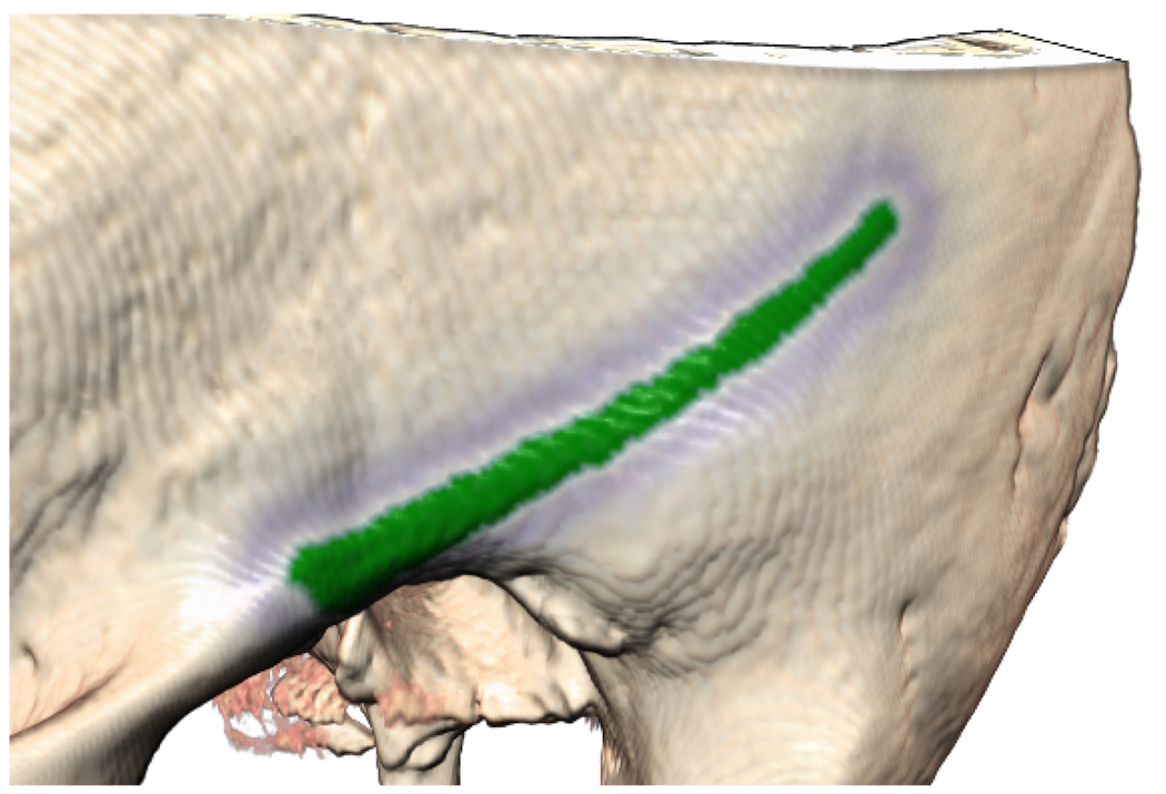
Since representation plays such a critical role in how well an individual perceives the form, structure, and organization of anatomical relationships, we allow expert users to highlight anatomical regions in different ways. The representations can be selected to accentuate a structure’s shape, border, edges, etc. to emphasize the structure or arrangement at issue. Specific areas on surfaces may have functional interest, meaning they delineate an area to commence surgical technique. For example, the temporal line (Fig. 6) is an important external landmark in determining where to start drilling in a basic mastoidectomy procedure. Structures embedded inside other structures can be more difficult to learn. Here volume visualization methods provide clarity through sectioning planes and transparency. A student must be able to mentally “visualize” what to expect while following a surgical trajectory through layers of tissue, considering what structures will be encountered along the way and in what order. For example, the lateral semicircular canal is a deep landmark that identifies the edge of the vestibular system. This structure is very important to locate and avoid during the surgery. Our application uses the WDT to provide sophisticated images to those learning the locations of these and other critical structures. We describe the distance transform in Sec. 3 and the visualization techniques using the weighted and unweighted versions of the transform in Sec. 4.

Figure 6.

The temporal line is highlighted in green and outlined in blue.

2 Related Work

Altering the color and opacity of data points with transfer functions is a powerful tool in the field of scientific visualization and it has an important place in the toolbox of volume visualization. There are many examples of using quantities derived from the primary scalar field in a dataset in order to render more complex and informative images, such as those demonstrated by Kniss et al. [KKH02]. It is now common to use two-dimensional transfer functions to explore derived quantities using visualization tools. Simple quantities such as gradient magnitude and curl have been joined by more complex ones, such as a local size property, as shown by Correa and Ma [CM08] and textural features, as shown by Caban and Rheingans [CR08]. Our system takes a similar approach: defining a distance property and using multiple rendering equations and transfer functions based on that property to present informative images. However, these two articles focus on finding new features with exploratory visualization techniques, either looking at objects at a certain scale or with certain statistical features. Our work focuses on viewing segments that have already been determined and creating descriptive visualizations for them.

Our work shares goals with other importance-driven volume visualization systems, such as those of Burns et al. [BHW*07], Viola [Vio05], and Bruckner et al. [BGKG06]. These systems use a function on the data to determine an importance value. They then use this importance value for the manipulation of opacity through transfer function editing and clipping. This approach provides the capacity to more easily visualize anatomical structures inside opaque datasets. Their technique changes the opacity values depending on the viewpoint. This can be a good thing, but it trades off continuity of the image while viewing. Similarly, systems like those described by Svakhine et al. [SES05] have shown the power of location-based transfer functions to produce illustrative renderings. However, in that system, locations were defined by the user independently of the data: there was no way to automatically determine complex regions of interest. Our method uses segmented data to automatically generate regions of interest by allowing the user to choose a segment to produce more focused results.

Tapenbeck et al. [TPD06], Zhou et al. [ZDT04], and Shinobu et al. [MiKM01] all used the concept of distance fields in volume rendering. This paper expands their work with multiple techniques using the more generalized concept of a weighted distance field. Tappenbek et al. used distance fields with two-dimensional transfer functions to minimize occlusion in medical volume rendering. However, the context for a particular rendering has to be defined manually. By using the weighted distance field, multiple levels of context can be defined automatically based on the anatomical data. Chen et al. [CLE07] use a uniform distance field of a volume segment to create exaggerated shapes for illustrative rendering. Felzenszwalb and Huttenlocher [FH04] have given a generalization to the distance field. In their formulation, instead of a binary input image, they use a scalar field to determine the degree of membership in the set to which the distance transform is applied. This corresponds to a modification of Eq. 2 in this article. To improve performance, Maurer et al. [MQR03] presented an algorithm to calculate the exact Euclidean distance transform in linear time. In work by Ikonen and Toivanen [IT07], the authors have provided an algorithm for a gray-level WDT that uses a priority queue. See Fabbri et al. [FCTB08] for a survey of Euclidean distance transform algorithms.

3 Distance Transform

The distance transform provides us with a convenient mathematical definition for determining the spatial relationships between a subset of a volume and every other voxel in the volume. In our case, the user chooses an anatomical structure by name and indicates the visual effect that should be applied. The name corresponds to a particular segment mask W that defines the voxels determined to be in that structure. The standard distance transform assigns every point g in space a real value equal to the minimum distance from g to a subset W of that space. Although the distance function is commonly defined on a ℝⁿ space, we present the discretized version here, since we are only concerned with voxel grids. Given a distance function d : ℤⁿ × ℤⁿ → ℝ, and a set W ⊂ ℝⁿ we can define a function D:

$$D:\{\begin{array}{cc}{\mathrm{\mathbb{Z}}}^n\hfill & \to \mathrm{ℝ}\hfill \\ \mathbf{g}\hfill & \mapsto {\text{min}}_{h\in W}(d(\mathbf{g},\mathbf{h})+c(\mathbf{h},W))\hfill \end{array}$$ (1)

When D is applied to a scalar field, each location g in the field is assigned the minimum cost from g to h, where h has a base cost determined by the function c. The c(h, W) value is needed to determine a base cost for the voxels not in the set, otherwise the transformation would be undefined for voxels that can’t reach set W. This c is usually defined as a binary choice based on set ownership:

$$c(\mathbf{x},W)=\{\begin{array}{cc}0\hfill & \text{if}\mathbf{x}\in W\hfill \\ \infty \hfill & \text{otherwise}\hfill \end{array}$$ (2)

3.1 The Weighted Distance Transform

The distance transform is normally computed using a common distance function for d. This function is often defined as a metric, such as Euclidean or Manhattan distance. For a WDT, the cost for moving one voxel in the space is defined by a separate scalar field. In the standard case, d is not only a metric but also monotonic, as defined by Maurer et al. [MQR03]. Monotonicity is property that the distance field resulting from a monotonic function will decrease and then increase over the course of a line parallel to an axis. This property allows more efficient computation of the distance field, and many optimizations in the literature assume monotonicity.

We use a weighted distance transform, where d is not a metric. Therefore, we can not use any optimizations that rely on the monotonic property. We use the scalar density field f of the original scan to determine the weighted distance between two voxels. We define d(g,h) to be the total weight of the shortest path between g and h. The cost of going from adjacent elements a to b could be computed variously as |f(a) − f(b)| or max(f(b) − f(a), 0). We use the weight f(b) in our algorithms to better approximate the distance field as an emanation from a source which is being impeded to a degree represented by the scalar field. This is analogous to traditional raycasting through a scalar field, where the field value represents the opacity to light. Different weight functions combined with specialized transfer functions can be used to create different effects on the final visualization.

4 Transfer Function Design

An important part of any anatomical visualization program is the ability to clearly show anatomical structures embedded in bone. As mentioned in Sec. 2, several approaches have been suggested previously, involving automatic clipping or defined areas of interest. With predefined structures, such as we have in professionally hand-segmented datasets, we can automatically generate interactive renderings of a selected structure along with the immediate context of nearby structures and far context of the rest of the dataset.

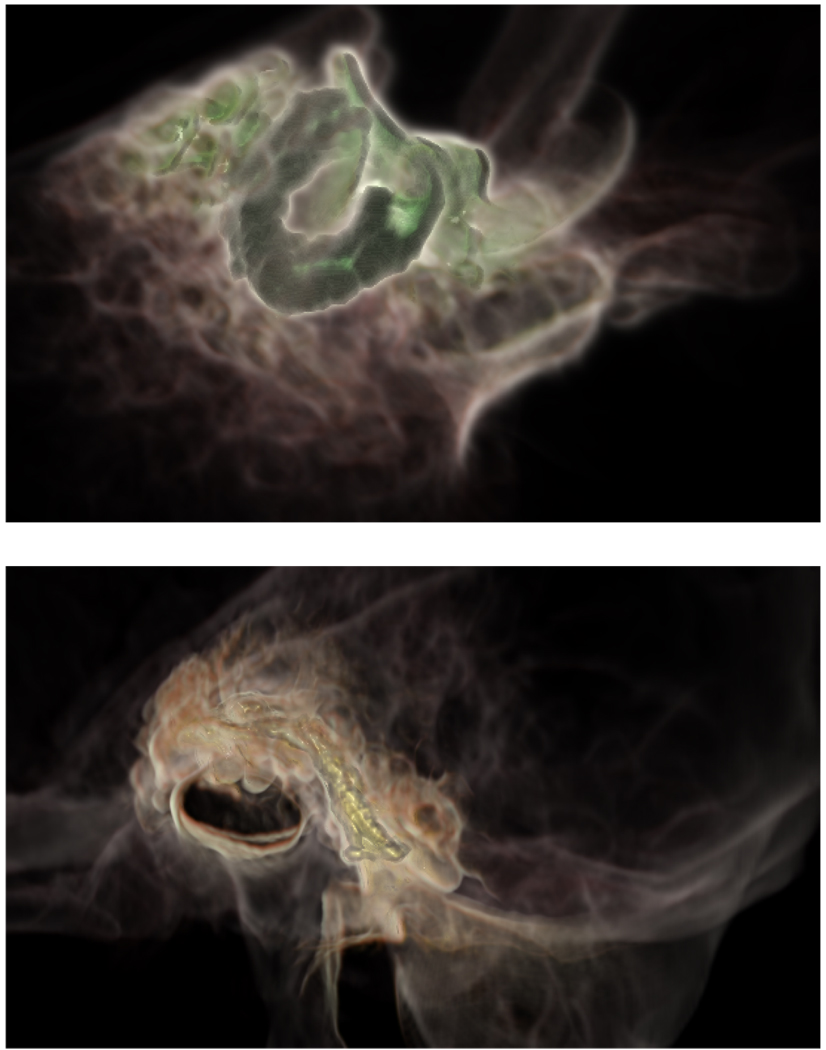
With a similar dataset and by manipulating the TF, we can use the WDT to easily show the relationship of embedded structures. Areas near the highlighted structure that are accessible without traveling through voxels that represent dense bone will have a higher value in the distance field than those that are behind thick bony masses. For example, in Fig. 2a, the posterior semicircular canal is highlighted. This structure, located in the skull and assisting with balance, is surrounded by bony structures and can be hard to visualize without selective transparency or a clipping plane. By using a distance-based TF, we can generate an image which shows the local bony structures and parts of the neighboring semicircular canals along with nearby air cells in the bone. Similarly, in Fig. 2b, and Fig. 1, segments are highlighted and a TF is used to create a semitransparent surface a certain distance away from the structure.

Figure 2.

The application highlights the chosen anatomical structures, fading out based on the density of bone. This allows the user to more easily see the bone structure near such embedded structures as the posterior semicircular canal (top) and the facial nerve (bottom).

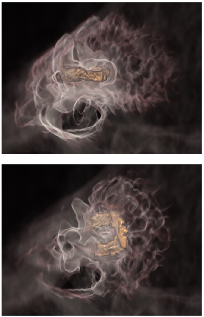
Figure 1.

Weighted distance field rendering for the lateral (top) and posterior (bottom) semicircular canals. The selected structures are rendered in high opacity orange, and nearby bony structures are rendered with a medium opacity white, fading opacity as the weighted distance from the structure increases.

Although a standard two-dimensional TF interface is certainly an option with this technique, we use a two-level interface with a higher dimensional TF constructed from two one-dimensional TFs. This interface consists of an expert level where the TFs are designed and a basic level where the TFs are loaded and used to view the data.

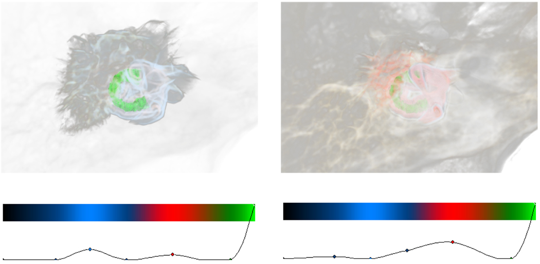
In the expert level interface, the user edits both the data and distance TFs using a spline based interface. The distance TF can be seen in Fig. 3, and the data transfer function is controlled the same way. After selecting a structure to view and setting these parameters, the expert user saves the parameters as a preset. In the basic level interface, the user loads a preset and uses a slider to blend between the data and the distance TF according to Alg. 1. The slider controls t, which goes from 0 to 1.

Algorithm 1.

Create 2D transfer function t f from 1D transfer functions dist and data using blend parameter t. LERP is linear interpolation with the interpolant as the last argument.

1: for all (i, j) do

2:   κ ← dist[j]A

3:   t f[i, j]RGB ← LERP(data[i]RGB, dist[j]RGB, dist[j]A)

4:   t f[i, j]A ← LERP(t * data[i]A, data[i]A * dist[j]A, κ)

5: end for

Figure 3.

By modifying the distance TF, the user can control the display of context both nearby and remote. The expert interface allows users to set opacities for distance values. Right clicking on a spline point allows color selection.

This 2D TF is then used to look up the final color value of each voxel based on the original data value and calculated distance field. To convert from a voxel-space distance field to a normalized value suitable for use in a texture lookup, we use an exponential function on each element of the field (x) with the user variable α controlling falloff:

$$f(x)=\frac{2}{1+{\alpha }^x}$$ (3)

4.1 Comparison with other methods

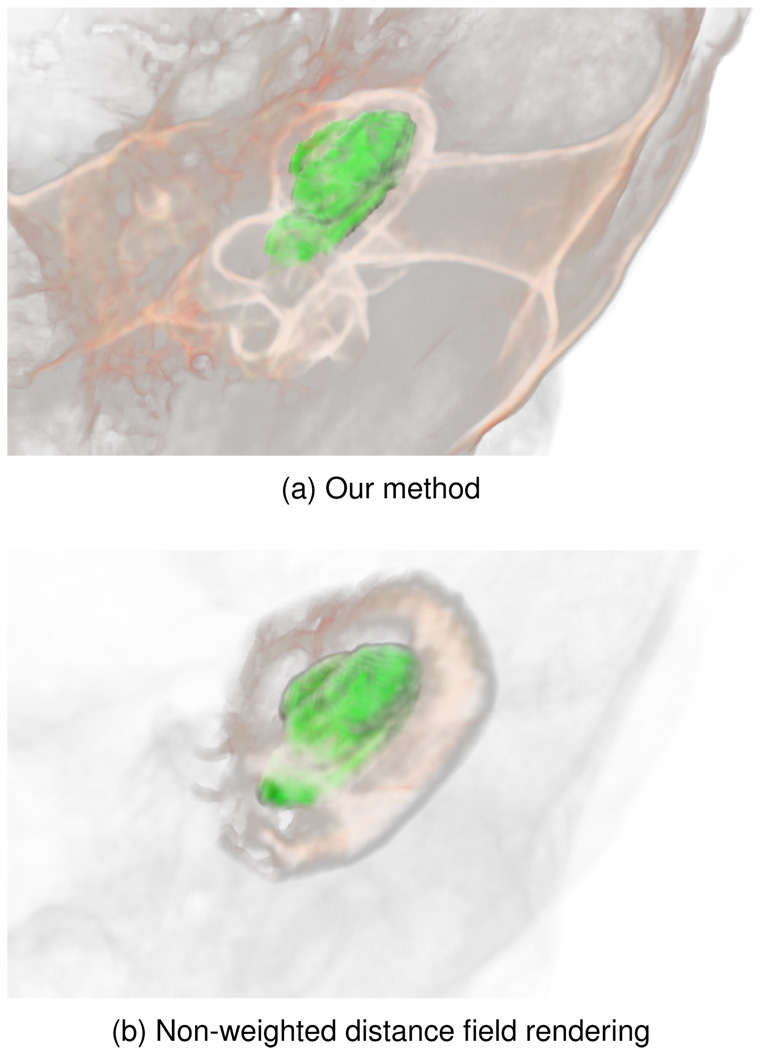
With a non-weighted distance transform, the resultant scalar field has no correlation to the original data, only to the segmented region. As can be seen in the lower image in Fig. 4, this can produce the effect of having clouds around the selected structure without providing any additional data to the viewer. By using a weight proportional to the opacity of the bone, we can show structures of the ear that are close to the cochlea. The upper image in Fig. 4 reflects the accessibility of voxels to the selected structure. This property leads to substantial benefits in final image quality when using a WDT rather than the non-weighted version. A transfer function based on distance from the centroid of a structure will give similar results to the non-weighted examples for compact structures, but for long, thin structures such as nerves and blood vessels, using a spherical effect will detract from visualizing the shape of the structure. Additionally, our method has an advantage over purely screen-space methods, as it can reflect the true 3D shape of the object in the visualization. Since the distance field is calculated per structure, no additional calculation is required per frame other than the transfer function application.

Figure 4.

The cochlea. Our technique highlights the nearby internal and external auditory canals. A non-weighted distance transform fails to emphasize any nearby structures.

4.2 Fuzzy edges

The boundaries of anatomical features often can not be determined directly by quantitative analysis of a data acquisition. In this type of situation, trained experts use their judgment aided by atlases to classify voxels as one structure or another. However, experts can disagree about the exact placement of the boundaries between structures. For example, a line dividing the hand and the arm could be placed differently by different medical professionals.

We can use the distance transform to generate images that accentuate the fuzzy nature of this type of boundaries. Using a simple transfer function to modify the color of the voxel based on the distance from the segment, we can give the segment soft boundaries that reflect the inherent lack of precision associated with the structure. These soft boundaries are generated per segment at run time and do not require a floating-point fuzzy segmentation by the anatomical expert. The amount of data required for storing fuzzy segments for a general segmentation approach can be quite large, although compression techniques like those described by Kniss et al. [KUS*05] can be used.

In this application of the distance field, we use a slightly modified lighting equation for each voxel:

$$C=K_d^{\prime }(n·l)+K_s{(r·v)}^s+K_a$$ (4)

$$K_d^{\prime }=K_d·(1-\mathit{\text{dist}})+K_h·\mathit{\text{dist}}$$ (5)

where K_h is the user specified highlight color and dist is a normalized distance factor between a voxel and the nearest selected structure voxel. The linear interpolation between colors is done in the XYZ color space in order to minimize known problems with RGB color arithmetic. In our system, K_h is determined by a real-time editable lookup table controlled by a 1D transfer function.

In our case, we employ CT acquisitions from skulls, both human and animal. The skull has many high level anatomical features that cannot be determined by analysis of the raw opacity values of the scan. For example, the boundary between the coronoid process and the rest of the ramus of the mandible is not a strict one: it has no grooves or suture lines to mark the division. The ramus is the vertical bony structure on the back of the mandible (jawbone), and the coronoid process is the upper part of the ramus.

Our technique is well suited to CT datasets, because the intensity values of the CT correspond naturally well to opacity values. We have tried MRI datasets and have not gotten results that were as easily interpreted by doctors and laypeople as from the CT. However, there is potential for a more complex transfer function to deliver informational imagues with our approach with different modalities.

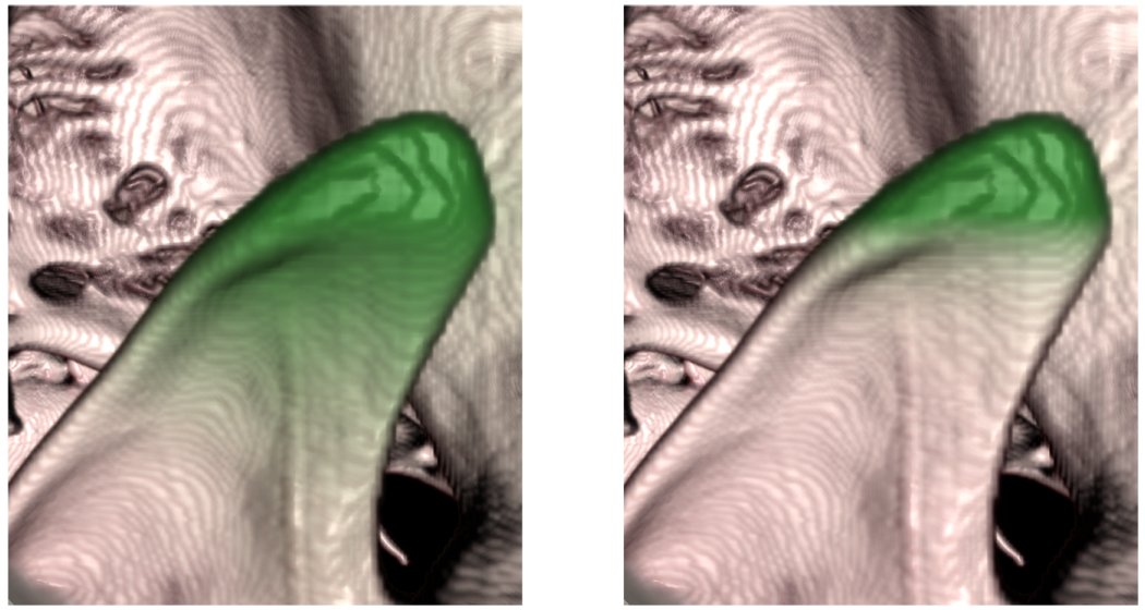
Fig. 5, shows the difference between using a simple binary mask for coloration of the segment and using a distance-based technique. With the addition of the distance field, the fuzzy boundary between the coronoid process and the lower ramus is more apparent. Using a different transfer function that peaks at a higher distance, we can create automatic outlining of structures. In Fig. 6, such a transfer function has been used to outline a segment on the side of the skull. A thin outline in this case represents an isosurface in the distance field and by setting different filters on the distance field, we can generate thin, thick, fuzzy or hard-edged outlines. By manipulating the transfer function, an illustrator could introduce differently styled lines for different purposes.

Figure 5.

The coronoid process is highlighted in green. In the left image, our technique shows a gradual change of color near the structure, emphasizing that the exact definition of the boundary line is subjective. The right image shows traditional hard-edged segment rendering.

This type of outline highlight can be useful in illustrative rendering when demonstrating a safety boundary in surgical applications. For example, since the density of bone is reflected in the boundary placement, the outline is further from the structure where the bone is less dense. This corresponds to a larger area of bone that a surgeon must be cautious about, since a bone drill penetrates lower density bone more quickly than dense bone.

4.3 Internal Volumetric Lighting Effects

The incorporation of global illumination techniques into volume rendering can improve image quality and give a better sense of shape and space to the objects represented in the rendering. Using a weighted distance field, we can approximate ambient occlusion effects for light sources inside of the volume. We can view the highlighted segment as a light source and the value of the distance field at each point as the amount of illumination that travels through that point. The contribution that the ambient light provides to the total illumination at each voxel is calculated by an inverse square law. The function used is shown in Eq. 6. D is the value of the distance field at a voxel while α and β are scaling factors that can be adjusted to account for the size of the dataset and the intensity of the light.

$$k_a=\frac{\beta }{{(\alpha D+1)}^2}$$ (6)

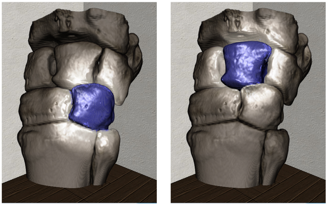
We can use this position dependent k_a factor instead of the normal constant k_a in the Phong rendering equation to render images with ambient lighting based on the length of the path from each voxel to the nearest light source. Since the WDT determines the weights from the density values of the voxels, the rendered image reflects light passing through translucent parts of the volume and structures that have been set to full transparency by a user transfer function. See Fig. 7 for an example of this technique. By computing the weighted distance field from voxels deemed to be light sources, we can compute an approximation of the ambient contribution of the light at every point in the volume.

Figure 7.

The hamate (right) and lunate (left) bones are highlighted using volumetric lighting. The distance field is used to calcuate an estimate for the amount of illumination going from the selected bone to the rest of the scene.

5 GPU calculation of the distance transform

Determining the distance transform can be expensive with large volumetric datasets. As mentioned in Sec. 2, there are many algorithms that provide good running times. However, many of these techniques are not applicable to the WDT, since they assume the distance metric used to be monotonic. To increase performance, we perform the calculation of the distance field in CUDA.

Since our applications require us to quickly update our distance field for the user during visualization, we compute an estimation of the weighted distance field using a multiaxis sweeping algorithm which propagates the field through the data. With a volume containing X³ voxels, each sweep has a O(X³ · p⁻¹) running time, where p is the number of processors on the GPU, assuming optimal hardware utilization. We perform six sweeps, one forward and one backward in each of the primary axes. We present the algorithm for sweeping forward along dimension X in Alg. 2. The algorithm for the Y and Z dimensions are similar.

We can perform additional sweeps to increase the accuracy of the field as needed. This algorithm eventually converges to the true Euclidean distance field, although this is not necessary for our purposes. With the application of only a couple sets of sweeps of the volume we obtain a distance field that is sufficient for our visualization requirements. The images in this article are all generated from distance fields produced by either six or twelve sweeps through the data.

Algorithm 2.

Sweep along dimension X

1: for all (y, z) in plane P perpendicular to X do

2:  x ← 0

3:  while x < length of volume in X do

4:    d ← ∞

5:    for all voxels v adjacent to voxel(x,y,z) do

6:      d ← min(d, dist(v, voxel(x,y,z))

7:    end for

8:    voxel(x,y,z) ← d

9:    x ← x + 1

10:  end while

11: end for

6 Performance and Results

While the focus of this work is not to present an improved algorithm for calculating the WDTs on a GPU, we present some timing information here to show that the system can generate new distance fields on user request rapidly enough to allow an interactive session with the software. Therefore, no preprocessing and storage of the distance fields is needed for the system: only the original CT data and the segmentations are needed. In Table 1, we give performance information for three datasets of various sizes. The time taken to regenerate the distance depends on the size of the volume. The tests were performed on a quad-core Core 2 Duo with 2GB of system memory with a NVIDIA GeForce GTX 280 with 1GB of graphics memory. In one application we have the user select the segment from a list and run the distance field algorithm as needed based on the user parameters. From our experience, a second or two is an acceptable amount of time in this situation and does not cause frustration on the part of the user. This is because the delay is only on selection of a new structure and does not impact rendering framerates.

Table 1.

Performance of the distance transform for various datasets. The number of passes refer to total runs of the algorithm: scanning through each dimension of the volume two times.

Dataset	Temporal Bone	Horse Knee	Cat Skull
Dimensions	256×256×256	332×291×354	384×288×528
Number of Voxels (in millions)	16.8	34.2	58.4
Average time calculating distance, 1 pass (in seconds)	0.30	0.48	0.9
Average time calculating distance, 2 passes (in seconds)	0.56	0.88	1.6
Average rendering FPS	20	19	17

However, a user interface design decision in a particular anatomy testing application was to have the user highlight segmented regions by moving the mouse over them. In this case, we found the half-second delay caused significant user frustration. To improve the speed, we ran the distance transform on a smaller sized volume. Using the down-sampled distance transform while keeping the full size for the original CT data in rendering proved useful. Reducing the size of the computed distance field by an eighth reduced the time needed to compute it by around an eighth as well, and this was sufficient for our users. As the accompanying video shows, the rendering is done in real-time with interactive framerates. A short pause is necessary to change structures, but after the distance field is computed, lighting parameters and transfer functions can be changed with their results immediately shown on the screen.

We asked 19 people to use the anatomical application and complete a survey. As discussed in Sec. 4, they did not manipulate the transfer function, but were given presets. There were thirteen seperate structures that each had two presets: one displayed a distance field rendering and another displayed the bare structure. They were asked try the different presets to visualize the structures, and then to answer a survey about the two different classes of presets. The survey included questions that asked the users if they thought the distance field rendering presets or the traditional bare structure rendering presets were better for various tasks. The results of the survey are shown in Table 2. All of the subjects found the preset and slider system straightforward to use and found the framerates sufficient. There were very few questions about the user interface after an initial explaination.

Table 2.

The chart plots the average user preference between two rendering techniques for three different applications and overall utility. A value of 1 was given for WDT rendering and a value of 5 was given for traditional segment rendering (TSR). A value of 3 indicates equal preference. The WDT technique was generally prefered except for showing the shape of the structure.

		Non-Medical users				Medical users
Showing shape	3.6	Prefer WDT		Prefer TSR	3.5	Prefer WDT		Prefer TSR
Showing context	1.5	Prefer WDT		Prefer TSR	2.0	Prefer WDT		Prefer TSR
Localizing structures	2.6	Prefer WDT		Prefer TSR	2.3	Prefer WDT		Prefer TSR
Overall utility	2.5	Prefer WDT		Prefer TSR	2.3	Prefer WDT		Prefer TSR

Fifteen subjects had little or no medical training, and represented people starting medical education. They found the WDT rendering superior to a bare structure rendering for showing the context of a structure and showing relationships between structure. However, they found the traditional rendering of a structure with no distance field better for showing the shape of the structure. From dialog with the participants and comments they gave us, we found that although most of them preferred the WDT rendering, they thought seeing the bare structure with no context was important for understanding the shape of that structure.

Four of the subjects have M.D. degrees. In general, their scores were similar with the results from the non-experts. One of the experts thought both the WDT rendering and the bare segment rendering were inferior to setting the opacity to full and using the clipping plane exclusively. However, all of the experts found that the system was better than other methods of learning that they have used previously.

7 Conclusion

This paper presents novel uses for the weighted distance transform in volume visualization. We have used the weighted distance transform to create an application that can have benefits in teaching students not only the position of structures but also their relationship to other parts of the body. In addition to displaying semi-transparent data, we can use the weighted distance transform for ambient lighting. Although the distance field is not as accurate as a photon mapping or more sophisticated system of ambient light calculation, it can be computed much more quickly than those systems. We have only used one function to define the distance field, but as shown in Sec. 3.1, there are many options for picking alternative functions.

In general, the weighted distance transform can be used for a wide number of effects to improve anatomical visualization. These effects are used in our application to show context and location of structures both in and on the skull and other body parts.

References

- [BGKG06].Bruckner S, Grimm S, Kanitsar A, Gröller ME. Illustrative context-preserving exploration of volume data. IEEE Transactions on Visualization and Computer Graphics. 2006 Nov;12(6):1559–1569. doi: 10.1109/TVCG.2006.96. [DOI] [PubMed] [Google Scholar]
- [BHW*07].Burns M, Haidacher M, Wein W, Viola I, Gröller E. Feature emphasis and contextual cutaways for multimodal medical visualization. Euro-Vis 2007. 2007 May;:275–282. [Google Scholar]
- [BKW08].Bürger K, Krüger J, Westermann R. Direct volume editing. IEEE Transactions on Visualization and Computer Graphics. 2008 November–December;14(6):1388–1395. doi: 10.1109/TVCG.2008.120. [DOI] [PubMed] [Google Scholar]
- [CLE07].Chen W, Lu A, Ebert DS. Shape-aware volume illustration. Comput. Graph. Forum. 2007;26(3):705–714. [Google Scholar]
- [CM08].Correa C, Ma K-L. Size-based transfer functions: A new volume exploration technique. IEEE Transactions on Visualization and Computer Graphics. 2008;14(6):1380–1387. doi: 10.1109/TVCG.2008.162. [DOI] [PubMed] [Google Scholar]
- [CR08].Caban JJ, Rheingans P. Texture-based transfer functions for direct volume rendering. IEEE Transactions on Visualization and Computer Graphics. 2008;14(6):1364–1371. doi: 10.1109/TVCG.2008.169. [DOI] [PubMed] [Google Scholar]
- [FCTB08].Fabbri R, Costa LDF, Torelli JC, Bruno OM. 2d euclidean distance transform algorithms: A comparative survey. ACM Comput. Surv. 2008;40(1):1–44. [Google Scholar]
- [FH04].Felzenszwalb PF, Huttenlocher DP. Distance Transforms of Sampled Functions. Tech. rep., Cornell Computing and Information Science. 2004 [Google Scholar]
- [IT07].Ikonen L, Toivanen P. Distance and nearest neighbor transforms on gray-level surfaces. Pattern Recognition Letters. 2007;28(5):604–612. [Google Scholar]
- [KKH02].Kniss J, Kindlmann G, Hansen C. Multidimensional transfer functions for interactive volume rendering. IEEE Transactions on Visualization and Computer Graphics. 2002;8(3):270–285. [Google Scholar]
- [KUS*05].Kniss JM, Uitert RV, Stephens A, Li G-S, Tasdizen T, Hansen C. Statistically quantitative volume visualization. IEEE Visualization. 2005;37 [Google Scholar]
- [MiKM01].Mizuta S, Ichi Kanda K, Matsuda T. Volume visualization using gradient-based distance among voxels. MICCAI. 2001:1197–1198. [Google Scholar]
- [MQR03].Maurer CRJ, Qi R, Raghavan V. A linear time algorithm for computing exact euclidean distance transforms of binary images in arbitrary dimensions. IEEE Transactions on Pattern Analysis and Machine Intelligence. 2003 Feb;25(2):265–270. [Google Scholar]
- [SES05].Svakhine N, Ebert DS, Stredney D. Illustration motifs for effective medical volume illustration. IEEE Computer Graphics and Applications. 2005;25(3):31–39. doi: 10.1109/mcg.2005.60. [DOI] [PubMed] [Google Scholar]
- [TPD06].Tappenbeck A, Preim B, Dicken V. Distance-based transfer function design: Specification methods and applications. SimVis. 2006:259–274. [Google Scholar]
- [Vio05].Viola I. PhD thesis. Institute of Computer Graphics and Algorithms, Vienna University of Technology; 2005. Jun, Importance-Driven Expressive Visualization. [Google Scholar]
- [ZDT04].Zhou J, Döring A, Tönnies KD. Distance based enhancement for focal region based volume rendering. Proceedings of Bildverarbeitung für die Medizin. 2004:199–203. [Google Scholar]