Field-portable lensfree tomographic microscope

Abstract

We present a field-portable lensfree tomographic microscope, which can achieve sectional imaging of a large volume (~20 mm³) on a chip with an axial resolution of <7 μm. In this compact tomographic imaging platform (weighing only ~110 grams), 24 light-emitting diodes (LEDs) that are each butt-coupled to a fibre-optic waveguide are controlled through a cost-effective micro-processor to sequentially illuminate the sample from different angles to record lensfree holograms of the sample that is placed on the top of a digital sensor array. In order to generate pixel super-resolved (SR) lensfree holograms and hence digitally improve the achievable lateral resolution, multiple sub-pixel shifted holograms are recorded at each illumination angle by electromagnetically actuating the fibre-optic waveguides using compact coils and magnets. These SR projection holograms obtained over an angular range of ~50° are rapidly reconstructed to yield projection images of the sample, which can then be back-projected to compute tomograms of the objects on the sensor-chip. The performance of this compact and light-weight lensfree tomographic microscope is validated by imaging micro-beads of different dimensions as well as a Hymenolepis nana egg, which is an infectious parasitic flatworm. Achieving a decent three-dimensional spatial resolution, this field-portable on-chip optical tomographic microscope might provide a useful toolset for telemedicine and high-throughput imaging applications in resource-poor settings.

Introduction

Light microscopy continues to serve scientists as a vital tool to visualize the structure of micro-objects such as cells and multicellular organisms. Much research has been devoted to date to extend the capabilities of conventional light microscopy to acquire more useful information regarding the objects under inspection. In particular, tomographic imaging modalities that can provide volumetric structural information of objects with high resolution have experienced a rapid development over the last few years.^1–12 For example, optical projection tomography (OPT),^1,2 optical diffraction tomography (ODT)^3–8 and light-sheet microscopy^9,10 are among these recently developed optical tomography modalities that can be used for three-dimensional (3D) bright-field and fluorescent imaging of objects ranging from sub-micron to centimetre scale in size. Nevertheless, the size, the cost and the complexity of these optical imaging platforms have also continuously increased, which in general limits their use to advanced laboratories. On the other hand, there is an increasing need for field-deployable microscopes,^13–19 whose requirements are much different than those designed for use in advanced settings. Toward this end, we have recently demonstrated that lensfree on-chip imaging that is based on partially coherent digital in-line holography^16–19 can achieve sub-micron resolution over a wide field-of-view (FOV) of e.g., ~24 mm² within a compact, lightweight and cost-effective imaging architecture, which is especially suitable for telemedicine applications in resource-poor environments. The axial resolution of these lensfree field-portable microscopes, however, is still significantly lower (e.g., >45–50 μm) owing to the inherently long depth-of-focus of digital in-line holography in general.^20,21 Although lensfree optical tomographic microscopy based on micro-mechanical scanners in a bench-top platform has recently been introduced to achieve sectional imaging over a large volume with <3 μm axial resolution,²² a field-portable and cost-effective tomographic tele-medicine microscope has yet to be demonstrated.

Toward this end, here we present a field-portable lensfree tomographic microscope that can achieve depth sectioning of objects on a chip. This compact lensfree optical tomographic microscope, weighing only ~110 grams, is based on partially coherent digital in-line holography^16–19 and can achieve an axial resolution of <7 μm over a large FOV of ~20 mm² and a depth-of-field (DOF) of ~1 mm, probing a large sample volume of ~20 mm³ on a chip. By extending the DOF to ~4 mm, the imaging volume can also be increased to ~80 mm³ at the cost of reduced spatial resolution.

In this field-portable lensfree tomographic platform, the major factors that enable a significantly enhanced 3D spatial resolution are: (i) to record multiple digital in-line holograms of objects with varying illumination angles for tomographic imaging; and (ii) to implement pixel super-resolution through electromagnetic actuation to significantly increase the lateral resolution of lensfree holograms at each viewing angle. For implementation of this tomographic on-chip microscope, we used 24 light-emitting diodes (LEDs—each with a cost of <0.3 USD) that are individually butt-coupled to an array of fibre-optic waveguides tiled along an arc as illustrated in Fig. 1. In this scheme, since the diameter of each fibre core is ~0.1 mm, there is no need for a focusing lens or any other light coupling tool, which makes butt-coupling of each LED to its corresponding fibre-end rather simple and mechanically robust. To increase the temporal coherence of our illumination source, we narrowed the spectrum of the LEDs down to ~10 nm (centred at ~640 nm) using interference based colour filters (<50 USD total cost, Edmund Optics) mounted on a piecewise arc that matches the geometry of the fibre-optic array (see Fig. 1). After this spectral filtering, the coherence length of the illuminating beam increases to ~30 μm, which permits obtaining holograms with a numerical aperture (NA) of ~0.3 to 0.4 up to an object height of ~1 mm from the sensor-chip surface.¹⁹

Fig. 1.

A photograph (left) and a schematic diagram (right) of the field-portable lensfree tomographic microscope (weighing ~110 grams) are shown. 24 LEDs are butt-coupled to individual optical fibres, which are mounted along an arc to provide multi-angle illumination within a range of ±50°. LEDs are sequentially turned on by a micro-controller to record projection holograms of the objects. At each angle, multiple sub-pixel shifted holograms are recorded to synthesize projection holograms with enhanced numerical aperture and resolution. These holograms are digitally processed to first obtain projection images, and then to compute tomograms with <7 μm axial resolution over a large sample volume of ~20 mm³ on a chip.

As illustrated in Fig. 1, the sample to be imaged can be placed on a standard cover-glass, which is positioned on the top of the sensor array using a sample tray inserted from one side of our portable tomographic microscope. Since the sample is much closer to the active area of the sensor-array (e.g., <4 mm) compared to its distance to the light source (~60 mm), lensfree holograms of objects can be recorded over a wide FOV of e.g., ~24 mm², which is >20 fold larger than the FOV of e.g., a typical 10× objective-lens. A low-cost micro-controller is then used to automatically and sequentially switch on the LEDs (one at a time) to record lensfree projection holograms of the sample within an angular range of ±50° (see Video S1^†).

In order to perform pixel super-resolution (SR)^19,23 for enhancing our spatial resolution at each illumination angle, the fibre-optic waveguide ends are mechanically displaced by small amounts (<500 μm) through electromagnetic actuation as demonstrated in Video S2^†. In this scheme, the fibres are connected to a common bridge (arc-shaped plastic piece shown in Fig. 1) with low-cost neodymium magnets (radius: 3.1 mm, length: 6.2 mm) attached on both ends. Compact circular electro-coils (radius: 5 mm, height: 5 mm) are mounted inside the plastic housing, which are used to electromagnetically actuate the magnets (see the Methods section), resulting in simultaneous shift of all the fibres along both the x and y directions (see e.g., Video S2^†, where the coils are overdriven to make the shifts more visible to the bare-eye). It is quite important to emphasize that the exact amounts of displacement for these fibre-ends do not need to be known beforehand or even be repeatable or accurately controlled. As a matter of fact, the individual displacement of each fibre-end can be digitally calculated using the acquired lensfree hologram sequence.^19,23 Once the fibres are shifted to a new position by driving the coils with a DC current, a new set of lensfree projection holograms are recorded, each of which is slightly shifted in 2D with respect to the sensor array. A maximum current of 80 mA is required for the largest fibre displacement (i.e., <500 μm), with ~4 volts of potential difference applied across the electro-coil (50 Ω). Standard alkaline batteries (with a capacity of e.g., 3000 mA h) could be used to actuate the fibres without the need for replacement for at least several days of continuous use of the tomographic microscope. With the above described set-up, 10–15 projection holograms are recorded at each illumination angle to digitally synthesize one SR hologram for a given illumination angle (see Fig. 2(b1)–(b3)). These lensfree SR holograms are digitally reconstructed to obtain projection images of the samples (see e.g., Fig. 2(c1)–(c3)), which can then be merged together using a filtered back-projection algorithm^22,24,25 to compute tomograms of the objects located on the sensor-chip (see the Methods section for further details).

Fig. 2.

(a1–a3) Our hologram recording geometry is illustrated for three different angles of θ = −44°, 0° and 44°. (b1–b3) Pixel super-resolved (SR) projection holograms for the corresponding angles are shown. These holograms are cropped from a much larger FOV of ~24 mm². (c1–c3) Projection images obtained by reconstructing the SR holograms shown in (b1–b3) are shown for the corresponding angles. These projections are aligned to each other with respect to the bead at the centre of the images.

To validate the performance of this field-portable lensfree tomographic telemedicine microscope, we imaged micro-beads of different dimensions as well as a Hymenolepis nana egg, which is an infectious parasitic flatworm. Without utilizing lenses, lasers or other costly opto-mechanical components, the presented lensfree tomographic microscope offers sectional imaging with an axial resolution of <7 μm, while also implementing pixel super-resolution that can increase the NA of each projection image up to ~0.3 to 0.4,¹⁹ over a large imaging volume of ~20 mm³. Furthermore, this volume can also be extended up to ~80 mm³ (corresponding to a DOF of ~4 mm) at the cost reduced spatial resolution. Offering a decent spatial resolution over such a large imaging volume, this compact, light-weight (~110 grams) and cost-effective lensfree tomographic microscope could provide a valuable tool for telemedicine and high-throughput imaging applications in remote locations. And finally, our platform can also be integrated with microfluidic systems towards building an opto-fluidic tomographic on-chip microscope by utilizing the controlled flow of the objects through micro-channels.

Results

Initially we investigated the improvements brought by the implementation of pixel super-resolution techniques in our portable lensfree tomographic microscope. Fig. 3(b) shows a digitally synthesized pixel super-resolved (SR) hologram of a 2 μm diameter micro-particle, where holographic fringes with much higher spatial frequencies can now be observed when compared to a raw lower-resolution (LR) hologram shown in Fig. 3(a). As a result of this increased numerical aperture (NA), the reconstructed images using SR holograms exhibit higher lateral resolution as revealed by the visual comparison of Fig. 3(a3) and (b3), where (with SR) the 2 μm bead is imaged much closer to its actual size. Further, the line profiles along the x and y directions in Fig. 4(b) and (c) show that the FWHM of the holographically reconstructed 2 μm bead image reduces from 3 μm down to 2.2 μm using pixel SR, demonstrating the enhancement of NA in SR holograms compared to raw LR holograms.

Fig. 3.

(a) A measured low-resolution (LR) vertical projection hologram for 2 μm diameter micro-particles. (b) The digitally synthesized pixel super-resolved (SR) hologram for the same region, where holographic fringes with much higher frequencies can be observed, that are normally undersampled in (a). (a1 and a2) The y–z and x–z cross-sections for a micro-particle obtained by reconstructing the LR hologram in (a). (a3) The reconstructed image of the same micro-particle in x–y plane using the LR hologram shown in (a). (b1 and b2) The y–z and x–z cross-sections for the same micro-particle obtained by reconstructing the SR hologram in (b). (b3) The reconstructed image of the micro-particle in x–y plane using SR hologram shown in (b). (c1–c3) The sectional images (tomograms) through the centre of the micro-particle in y–z, x–z and x–y planes, respectively.

Fig. 4.

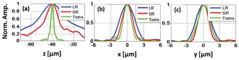
(a–c) Comparison of the line profiles along z, x and y, respectively, through the centre of a 2 μm diameter micro-particle image, obtained by reconstructing a single LR hologram (blue curves), an SR hologram (red curves) and by tomographic reconstruction (green curves).

Next we investigated the reconstructed depth (z) profiles corresponding to the LR and SR holograms shown in Fig. 3(a) and (b), respectively. By digitally reconstructing¹⁶ the LR lensfree hologram of Fig. 3(a) at several different depth (z) values, we can get the y–z and x–z profiles shown in Fig. 3(a1) and (a2) corresponding to the same 2 μm particle. In these results, the broadening along z illustrates the limitation of a single LR hologram toward depth sectioning. This limitation is partially improved using the SR lensfree hologram as illustrated in Fig. 3(b1) and (b2) and 4(a). On the other hand, despite the numerical aperture improvement with SR, it still does not permit sectional imaging of the objects with an axial resolution of e.g., ~45 μm or better. To mitigate this fundamental axial resolution limitation, we utilized lensfree SR holograms that are synthesized for ~20 illumination angles spanning a range of ±50° to create a tomogram of the same micro-particle as illustrated in Fig. 3(c1)–(c3) (refer to the Methods section for details). These results presented in Fig. 3 indicate that our field-portable lensfree tomographic microscope (Fig. 1) significantly improves the axial resolution, which can be observed by the shortened depth-of-focus of the bead image. According to Fig. 4(a), the full-width-at-half-maximum (FWHM) of the axial line profile for the same micro-particle is reduced from ~90 μm (for a single LR hologram) to ~45 μm by pixel super-resolution, which is then further reduced down to ~7.8 μm by our tomographic reconstruction. As a result, our field-portable tomographic microscope improves the axial resolution by a factor of >13× and ~6–7× compared to what is achievable with a single LR hologram and a single SR hologram, respectively.

Also note that the FWHM of the line profiles along the x and y directions for the computed tomograms, shown by Fig. 4(b) and (c), are 1.7 μm and 2.3 μm, respectively. The fact that the FWHM value along the x direction is smaller than the diameter of the particle is due to the well-known artefact in limited angle single-axis tomography,^26,27 where the main lobe of the point-spread-function (PSF) gets narrower along the direction of the source tilt. Similarly, the axial elongation of the PSF along the z direction is also partially due to the limited angular range of our illumination (i.e., ±50°), which degrades the axial resolution compared to the lateral. These artefacts can be minimized by using iterative back-projection algorithms²⁶ as well as by using a dual-axis tomography scheme where two sets of projection images are obtained by tilting the illumination along two orthogonal axes.^22,26

To further demonstrate the depth sectioning capability of our field-portable lensfree tomographic microscope, we imaged 5 μm diameter spherical micro-beads (refractive index ≈ 1.68, Corpuscular Inc.) that are randomly distributed within a ~50 μm thick chamber filled with an optical adhesive (refractive index ≈ 1.52, Norland NOA65). Fig. 5 shows the tomographic reconstruction results for a small region of interest that is digitally cropped from a much larger image area to match the FOV of a 40× objective lens (NA: 0.65) that is used for comparison purposes. These lensfree tomograms for the entire chamber depth were computed within <1 min using a Graphics Processing Unit (NVidia, Geforce GTX 480). Arrows in Fig. 5(b1)–(b5) indicate micro-beads that are in focus at the corresponding depth layer of the image, which can also be cross-validated using conventional microscope images that are acquired at the same depths as shown in Fig. 5(a1)–(a5). To further quantify our tomographic imaging performance, in Fig. 5(c) we show x and y line profiles for an arbitrary micro-bead located within the same FOV, where the full-width-at-half-maximum (FWHM) of the particle can be calculated as ~5 μm and ~5.5 μm along x and y directions, respectively, very well matching with its diameter (5 μm). The axial line-profile of the same bead tomogram (along the z direction) has a FWHM of ~12.9 μm as seen in Fig. 5(d) with the blue curve. It is important to note that, without the use of multi-angle illumination and tomographic digital reconstruction, using just a single SR hologram, the computed image of the same micro-particle would have an axial FWHM of >75 μm, which is expected for an in-line holographic imaging platform due to its long depth of focus. Following a similar approach as in ref. 3 and 4, by taking one-dimensional spatial derivative of the axial line-profile shown in Fig. 5(d) (i.e., the blue curve), the FWHM of the point-spread function of our tomographic microscope along the z direction can be estimated to be ~6 μm (refer to the red curve in Fig. 5(d)).

Fig. 5.

(a1–a5) The microscope images (40×, 0.65-NA) for different depth sections of a chamber filled with randomly distributed micro-beads with 5 μm diameter. (b1–b5) Our lensfree computed tomograms for the corresponding layers, which demonstrate successful depth sectioning with our tomographic microscope. The arrows in each image show the beads that are in-focus at a given depth. (c) A zoomed tomographic image through the centre of an arbitrary bead together with its line profiles along x and y. (d) The axial line profile and its derivative for the same bead as in (c), suggesting an axial resolution of ~6 μm. The inset in the figure, enclosed with the dashed rectangle, shows sectioning of two axially overlapping micro-beads, shown by the dashed circles in (a1) and (b5), both by lensfree tomography and conventional microscopy (40×, 0.65-NA). Notice that at z = 12 μm plane (shown at the centre of this inset) our lensfree tomographic image does not show anything since z = 12 μm refers to the depth layer that is between the two axially overlapping beads. This provides an independent validation for our significantly improved depth resolving capability. See Video S3^† for tomograms of other depth sections within the full FOV of the sensor-array.

Although Fig. 5 presents sectional images for a small region of interest, tomograms for the entire FOV can be computed without a significant change in the imaging performance. This is demonstrated in Movie S3^†, which shows tomograms for three different regions within a large FOV. Note that while all the recorded lensfree holograms have an effective FOV of ~24 mm², the reconstructed FOV for tomographic images reduces to ~20 mm² as the holograms of the objects that are close to edges of the active area of the sensor-array start to shift out of the chip area at large illumination angles.

Our lensfree hologram recording geometry shown in Fig. 1 has several advantages especially toward high-throughput imaging needs, achieving both a long depth-of-field (e.g., ~1 to 4 mm) and a wide field-of-view (e.g., ~20 mm²). In specific, lensfree holographic projections can be reconstructed at any depth of interest; and the tomograms can then be computed around that depth region without introducing spatial aberrations. This approach enables 3D imaging of any arbitrary region of interest within a long depth-of-field and hence a large imaging volume.

To specifically demonstrate this capability, we imaged a multilayer chamber (four layers stacked together with ~1 mm separation in between, i.e., a total thickness of ~3.5 mm) that is composed of 10 μm beads embedded in an optical adhesive. This thick object is placed at ~0.7 mm away from the active area of the sensor-chip with its furthest layer situated at z ≈ 4.2 mm from the sensor plane. Fig. 6(c1)–(c5) show the computed tomograms of different layers within this thick object, which demonstrate optical sectioning capability of our lensfree tomography approach within a long DOF. Tomograms of the entire DOF and the object volume can then be obtained by digitally merging such separate tomograms calculated at different layers. Lensfree holograms of the objects in the furthest layer (~4.2 mm away from the sensor) shift out of the sensor active area for illumination angles above 40° and below −40°, as a result of which our angular range was limited to ±40° only for the top layer (see Discussion section for details). We should also briefly note that the digital implementation of our pixel super-resolution scheme for tomographic imaging of thick or multilayer chambers requires additional signal processing since objects located at significantly different depths exhibit large variations in lateral shifts of their corresponding holograms at the sensor-plane as function of source shift. To handle this complication, we developed an iterative algorithm such that super-resolved holograms can be specifically calculated for a given depth layer (independent of the other layers) as illustrated in Fig. 6(b1)–(b3) (refer to the Methods section for further details).

Fig. 6.

The tomographic imaging performance for a multilayer chamber (mounted with 0.7 mm elevation above the sensor) of 10 μm beads, suspended over 4 layers with a total thickness of ~3.5 mm. (a) A recorded hologram of this multi-layer object, where the holograms of beads at different depths are visible (with varying sizes as a function of the distance from the sensor-chip). (b1–b3) Digitally cleaned holograms, which comprise the information of objects in only a selected layer, are shown (see the Methods section for details). (c1–c5) Computed tomograms for different depths are shown to demonstrate depth sectioning over a large DOF of ~4.2 mm.

And finally, in order to validate the performance of our field-portable lensfree tomographic microscope for potential applications in bio-medicine, we also imaged a Hymenolepis nana (H. nana) egg, which is an infectious parasitic flatworm of humans having an approximately spherical structure with ~40 μm diameter. Due to the long depth-of-focus of lensfree inline holography, optical sectioning of this egg is not possible by merely reconstructing its recorded hologram at any given illumination angle. However, as demonstrated in Fig. 7, separate depth sections of this parasite egg can be created using our tomographic handheld microscope (shown in Fig. 1), exhibiting distinct details/features at each depth layer.

Fig. 7.

(a1–a3) The computed tomograms for different depths of a H. nana egg, which can also be compared against 40× microscope images shown in (b1–b3). See Video S4^† for other depth sections of the same egg, which suggest a total thickness of ~40 μm, very well matching with its diameter.

Video S4^† further illustrates other sectional images of the computed tomogram for this object, from which the thickness of the parasite egg can also be deduced to be ~40 μm, providing a decent agreement to its diameter.

Discussion

Our field-portable lensfree tomographic telemedicine microscope achieves <7 μm axial resolution over a large imaging volume of ~20 mm³. The imaging volume can be extended up to ~80 mm³ at the cost of reduced spatial resolution at depths exceeding ~1 mm. Since the entire platform also lends itself to a compact and cost-effective architecture weighing only ~110 grams, our lensfree tomographic microscope can particularly be useful for telemedicine and high-throughput imaging needs for point-of-care or field use.

We should emphasize that the lensfree optical tomographic microscope presented here provides a unique approach for increasing spatial resolution without shrinking the field of view, which is a common trade-off in lens-based imaging systems. In our platform, bringing the sample close to the digital sensor array (<5 mm) while keeping the light source relatively distant (~60 mm) enables imaging a large FOV that is equal to the active area of the sensor chip (i.e., ~24 mm²). This unit fringe magnification scheme, however, poses a limitation for spatial resolution which is dictated by the pixel size.¹⁶ Nevertheless, pixel super-resolution techniques digitally enhance the lateral resolution of lensfree holographic on-chip imaging beyond this limitation¹⁹ up to an NA of ~0.4 to 0.5 over the same large imaging FOV. In addition to this, as demonstrated in this work, computed tomography with multi-angle illumination drastically improves the axial-resolution of field-portable lensfree microscopes^16–19 (from e.g. ~45 μm with SR down to <7 μm), without resulting in a significant reduction in the imaging FOV. Furthermore, our unit fringe magnification geometry also simplifies the illumination end of our portable tomographic microscope by permitting the use of a large aperture (e.g., an optical fibre with a core diameter of ~0.1 mm) such that without any coupling optics or sensitive alignment, a sufficiently large spatial coherence diameter can be created at the sensor plane. Consequently, projection holograms can easily be acquired using multiple light sources (i.e., cost-effective LEDs) located at different angles, as opposed to having to rotate the sample or the source mechanically, which could be quite expensive and challenging to practically achieve for a field-portable microscope.

The above described in-line holographic recording scheme with unit fringe magnification also relaxes the temporal coherence requirements at the source end. As a result, only a spectral bandwidth of ~5 to 10 nm is sufficient to reach a decent spatial resolution as demonstrated in this work and in our earlier results.¹⁹ Therefore, by choosing a sweet spot for both spatial and temporal coherence we significantly reduce the noise terms such as speckle and multiple-reflection based interference. Moreover, our limited coherence length also partially eliminates the undesired cross-interference among different depths of our imaging volume, which further reduces reconstruction artefacts since such cross-interference terms are entirely ignored in holographic reconstruction schemes.

It should also be noted that our tomogram FOV shrinks as the depth to be sectioned gets further away from the sensor chip. This is due to the fact that the holograms of the objects that are close to sensor edges do not fall onto the sensor chip at oblique illumination angles and shift out of the imaging FOV.²² Therefore, as the object is situated further away from the sensor, the FOV continues to get smaller resulting in a prismatic shape for the imaging volume that can be probed tomographically. For instance, if one wants to utilize the entire angular range of ±50°, the DOF would be limited to <3.5 mm, and the total imaging volume (corresponding to a triangular prism) would be ~42 mm³. In the multi-layer imaging experiment presented in Fig. 6, however, we utilized lensfree projections within ±40° of illumination angle for regions higher than ~3.5 mm from the sensor-chip, resulting in reduced axial resolution, and extended our DOF to ~4 mm, corresponding to an imaging volume of ~48 mm³.

In addition to the above discussed issue of angular range of illumination, at large object depths (e.g., z > 2–3 mm), the signal-to-noise ratio (SNR) of the recorded holograms will start to get lower (due to spatial spreading of the scattered fields), resulting in a reduced 3D resolution. Moreover, for such large object depths, the limited coherence length of our illumination (with a spectral bandwidth of e.g., ~10 nm) will also start to reduce the visibility of high frequency holographic fringes, limiting the achievable NA at each projection image.²² To mitigate this issue, an even narrower spectral filter (with e.g., 1–5 nm bandwidth) can be utilized to increase the contrast of such high-frequency fringes without the need for any other major changes in our tomographic microscope design.

The ability to create tomograms of objects distributed over e.g., 1–4 mm of depth is another unique aspect of our field-portable tomographic microscope. Such an extended DOF is directly enabled by our lensfree hologram recording geometry. Since the object wave is not collected through a high NA objective lens (which immediately restricts the DOF to e.g., <5–10 μm) lensfree holograms of objects over several millimetres of depth can be recorded all in parallel as long as the SNR is sufficiently high. On a related note, it should be clarified that an extended DOF of e.g., >1–4 mm demonstrated with our field-portable lensfree tomographic microscope should not be confused with the thickness of a continuous scattering object that can be optically sectioned. In computed optical tomography, in general, weakly scattering object assumption²⁸ is made such that the majority of the photons incident on the object encounters at most a single scattering event before being sampled at the detector plane (see the Methods section for details). Our field-portable lensfree tomographic microscope is also subject to the same assumption, and whether or not a given object satisfies this condition depends both on its scattering properties as well as its thickness.²⁹ Therefore, depth sectioning of a tissue slice, for instance, would not be feasible with the presented transmission based holographic tomography approach. For such a task, reflection imaging geometry could be more suitable rather than the transmission geometry of this work.

In this proof-of-concept demonstration of a field-portable tomographic microscope, we conducted experiments with static objects, i.e. non-moving samples. Nevertheless, our on-chip tomography system can also provide a useful toolset for lab-on-a-chip platforms. One approach to achieve integration with microfluidic platforms is to employ non-invasive immobilization of the objects by using special micro-fluidic trap designs^30,31 such that the objects of interest can first be captured, immobilized and then tomographically imaged, after which the flow can continue till the next imaging event. An alternative approach that we can take to image flowing samples is to digitally estimate the shifts and rotations of the objects, and incorporate this information in the digital reconstruction process. Along these lines, holographic optofluidic microscopy (HOM) has already been demonstrated by our group for 2D micro-fluidic imaging applications,²³ where lensfree in-line holograms are acquired as the objects are flowing within a microfluidic channel, and then are used to synthesize a single high-resolution (i.e., super-resolved) hologram of the objects. In other words, the flow of the object itself can be used, instead of moving the light source as demonstrated in this work, to record multiple sub-pixel shifted holograms. Using a similar approach in our portable tomography platform will not only pave the way toward an opto-fluidic tomographic microscope integrated with microfluidic systems, but may also simplify our approach further by eliminating the need for magnetically actuating the fibres to acquire sub-pixel shifted holograms, and utilize the controlled flow of the objects instead.

Finally, we would like to also note that the presented lensfree optical tomography scheme, which is based on multi-angle transmission holographic imaging, is not directly applicable to fluorescence imaging. To achieve lensfree 3D fluorescence imaging based on computed tomography, rotation of the object appears to be a more feasible approach. However, due to the limited depth-of-field of currently existing lensfree fluorescence microscopy techniques³² (e.g. <0.5 mm), imaging a large volume, as demonstrated in this work, would be challenging in lensfree fluorescence on-chip tomography.

Methods

Acquisition of lensfree projection holograms

Our field-portable optical tomographic microscope employs 24 LEDs that are individually butt-coupled to optical fibres, each with a core diameter of ~0.1 mm and a length of ~14 mm (see Fig. 1). These fibres are mounted along an arc such that they illuminate the sample from different angles, within a range of ±50° with ~4.1° increments. The spectrum of the LED illumination is narrowed down to ~10 nm (640 nm centre wavelength) using interference-based colour filters. Due to their angular sensitivity, 6 pieces of filters (~10 mm × 5 mm—cost per piece: <9 USD) are mounted in a way to form a piecewise arc that matches the geometry of the arc-shaped fibre array. This ensures near-normal incidence of light on these colour filters. We have observed, however, that the bandwidth of the filters do not change significantly (<1 nm) even for an incidence angle of ~20°. Therefore, quite conveniently the placement of the colour filters does not require any sensitive alignment with respect to the fibre tips.

In order to record lensfree projection holograms from multiple angles, these LEDs are sequentially and automatically turned on/off by a low-cost micro-controller (Atmel ATmega8515, ~3 USD per piece). A digital sensor array (Aptina MT9P031STC, 5 Megapixels, 2.2 μm pixel size), which is placed z₁ = ~60 mm away from the fibre-ends, records the lensfree projection holograms of the objects that are loaded (with z₂ < 5 mm distance to the active area of the sensor-chip) through a sample tray inserted from one side of the lensfree microscope (see Fig. 1). At each illumination angle, a series of sub-pixel shifted holograms are recorded for implementing digital pixel super-resolution.^19,23 For this purpose, all the fibres are mounted on a common arc-shaped bridge, which has neodymium magnets at both ends. By driving the coils mounted across these magnets with a DC current, electromagnetic force is generated that actuates the plastic bridge and simultaneously translates all the fibre-ends (refer to the Appendix for further details). These fibres are shifted to 10–15 different locations within a ~500 μm × ~500 μm grid, and for each position a new set of ~20 to 24 holographic projections are acquired. Note that such large shifts at the source plane correspond to much smaller shifts at the hologram plane because of the large z₁/z₂ ratio. More importantly, these shifts do not need to be accurate or repeatable since almost random shifts are equally valuable to achieve pixel super-resolution.^22,23 Further, there is no need for prior knowledge of these shifts since this information can be accurately obtained by processing the sequence of the acquired lensfree holograms.^19,23 Using a custom developed LabView (National Instruments) based auto-exposure software, a set of 24 images can be acquired in ~6 s at 4 frames per second, which can be significantly sped up using a sensor with a higher frame rate of e.g., >15–20 fps.

Despite the fact that the large z₁/z₂ ratio in our hologram recording geometry permits recording of holograms at angles close to ±90°, the design of digital sensor array itself restricts the actual range of illumination angles that can be used in our tomographic microscope. Most digital sensor arrays are designed for imaging systems that use lenses as imaging elements, as a result of which the angle of incident rays measured from the sensor surface normal is typically less than 20–30°. Therefore, the sensitivity of these opto-electronic sensors, by design, rapidly drops for incidence angles that are larger than 50° and aberrations become significant. Therefore, even though our hologram recording geometry permits the use of higher angles (e.g. 70–80°), we limit the angular range of illumination to ~50° for our tomographic microscopy set-up.

Digital processing of lensfree projection holograms to obtain projection images

The shifted holograms recorded at each illumination angle are processed similar to ref. 19 and 22 to synthesize projection holograms with higher spatial resolution. These digitally synthesized super-resolved holograms are then rapidly reconstructed to obtain lensfree projection images of the objects. Despite the use of oblique illumination angles, the object wave and the unperturbed reference wave propagate co-axially, and each lensfree hologram is still an in-line hologram.²² In order to eliminate the twin-image artefacts and recover the phase of the recorded optical field intensity, we use an iterative phase retrieval algorithm¹⁶ where the hologram field is propagated back-and-forth between the detector and object planes using the object support as a constraint during these iterations. Similar to conventional holographic reconstruction, the recorded hologram should be digitally multiplied by a reconstruction wave that is the digital replica of the reference wave utilized for recording the holograms. Therefore, prior to the iterative phase recovery steps, we first multiply the holograms with a plane wave that is tilted by an angle of θ_rec. It is also important to note that the tilt angle of this reconstruction wave, θ_rec, is not equal to the physical tilt of the illumination fibre due to the refraction of light within the sample chamber. In fact, θ_rec is determined by calculating the inverse tangent of the ratio Δd/z₂, where Δd denotes the lateral shift of the raw holograms with respect to their positions in the vertical projection hologram, and z₂ is either experimentally known, or is determined by the digital reconstruction distance of the vertical holographic images. Convergence is typically achieved in 10–20 iterations, after which the optical field in the object plane parallel to the detector is obtained. Nevertheless, this field needs to be rotated to obtain the projection image that is normal to the direction of illumination. To achieve that, the recovered field is interpolated on a new grid that is rescaled by cos(θ_rec) along the direction of the illumination tilt,^3,22 which effectively squeezes the recovered field, and provides the projection image for the corresponding angle.

Once the projection images at each illumination angle are calculated, they need to be registered with respect to a common centre-of-rotation before computing the tomograms (see e.g., Fig. 2(c1)–(c3) where the three projection images are aligned with respect to the bead at the centre). This is achieved by implementing an automated two-step cross-correlation algorithm. In the first step, the projection images for adjacent angles are aligned with respect to each other by cross-correlating the entire area of interest of these adjacent projections (e.g. 42° and 46°; 46° and 50°). Since the projection images for consecutive angles are very similar to each other, this operation provides an approximate initial alignment. However, this registration is not perfect due to slight changes of the scene as a function of viewing angle. In the second fine-alignment step, one of the projection images is selected as the global reference image, and all projection images are registered with respect to this reference image, but this time utilizing a smaller region of interest in the projections. This second step is especially required when aligning images of distributed small objects such as micro beads (see e.g., Fig. 2).

Calculation of super-resolved holographic projections for axially overlapping objects in a thick sample volume

For a chamber where the objects are distributed within a height of e.g., <200–300 μm, the holograms of all the objects shift almost equally for a given source shift. Therefore, a single SR hologram satisfying the measured data in all the sub-pixel shifted holograms can be synthesized.¹⁹ For thick or multilayer chambers, however, the lensfree holograms of objects that are axially separated by >200–300 μm shift considerably different amounts, and the recorded holograms for different source shifts look different. As a result, a single SR hologram to satisfy all shifted holograms cannot be calculated. To solve this issue, new holograms with the information of only the desired layers can be obtained by digitally erasing the undesired layers from the hologram intensity.²² To achieve that the lensfree hologram for a thick (or multilayer) chamber as in Fig. 6(a) is reconstructed at the undesired layers, and the objects that are focused at those layers are removed from the hologram field using a binary masking operation. Successively deleting all the layers except the desired one yields a new digitally cleaned hologram, which is faithful to the measured data for specifically the depth layer of interest. We have observed that erasing the layers that are closer to the sensor may leave residues in the cleaned hologram, but this does not pose any problems since these residues are quite weak, and the holograms for the desired layer are still completely in agreement with the originally measured raw holographic data. Finally, once these new holograms with different sub-pixel shifts are obtained for a given layer of interest, SR hologram of that depth layer can successfully be computed (see Fig. 6(b1)–(b3)) as described earlier.^19,22

Back-projection based reconstruction in lensfree optical tomography

The filtered back-projection algorithm^24,25 is utilized to compute tomograms of the objects from their lensfree projection images. A fundamental requirement for the validity of this approach is that the projection images should represent a linear summation of a property of the object^1,22,25 for which tomograms are being computed (e.g. phase, absorption, scattering strength, etc.). This is generally satisfied by weakly scattering objects^1,28 in which case the majority of the incident photons experience at most a single scattering event over the volume of the object.²⁹

Assume that a weakly scattering object is represented by a complex 3D scattering function s(x_θ,y_θ,z_θ), which satisfies |s(x_θ,y_θ,z_θ)| ≪ 1, where (x_θ,y_θ,z_θ) defines a coordinate system whose z-axis is aligned with the direction of illumination angle at a particular projection angle. In this case, the contribution of cross-interference terms to the hologram will be negligible in comparison to the actual holographic heterodyne terms. This assumption is further validated by the low spatial coherence (which minimizes cross-talk between objects with lateral separation larger than coherence diameter) and low temporal coherence (which minimizes the cross-talk between different layers with separation longer than coherence length) of our system, acting as a 3D coherence filter. As a result, for each projection image within a single tomogram volume (spanning e.g., Δz ≈ ±25 μm), the holographically reconstructed image contrast will yield the linear summation of the scattering strength function given by: ∫|s(x_θ,y_θ,z_θ)|dz_θ. Consequently, tomograms of scattering strength of an object can be computed by applying a filtered back-projection algorithm^22,25 whose inputs are the projection images calculated by holographic reconstruction of pixel super-resolved lensfree holograms acquired at various illumination angles, as we have demonstrated in this manuscript.

Conclusions

We presented a field-portable lensfree tomographic microscope weighing only ~110 grams, which can achieve depth sectioning of a large volume (~20 mm³) on-a-chip at an axial resolution of <7 μm. Furthermore, the imaging volume of this microscope can be extended up to ~80 mm³ at the cost of reduced spatial resolution. In the same compact platform, pixel super-resolution techniques are employed to significantly improve the numerical aperture of the recorded lensfree holograms. We evaluated the performance of this compact, light-weight and cost-effective lensless tomographic microscope by imaging various micro-beads as well as a Hymenolepis nana egg, which is an infectious parasitic flatworm. Imaging a large sample volume with a decent spatial resolution, this portable on-chip tomographic microscope might provide a useful tool for telemedicine and high-throughput imaging applications in field-settings.

Appendix

Design and electromagnetic actuation of the fibre-optic array for the portable lensfree tomographic microscope

As described earlier, the optical fibres that are used for multi-angle illumination are connected to a common arc-shaped lightweight bridge (~1.7 grams), which moves together with all the fibres when actuated by electromagnetic forces. The other ends of these fibre-optic cables are mechanically fixed and are butt-coupled to individually addressed LEDs. Therefore, the entire structure can be modelled as a spring-mass system, where all the fibres collectively act as a spring, and the bridge piece is the mass load.

There are several critical specifications that need to be taken into account for the design of this structure: (1) to keep the form factor of the instrument small, the overall architecture of the actuator should be as compact as possible; (2) the structure should be stiff enough to stay rigid by itself such that small external perturbations do not randomly move the fibre tips during image acquisition, which would otherwise cause blurring of the recorded holograms; (3) the natural mechanical resonant frequency of the lowest vibrational mode of the structure should be as high as possible such that the structure does not move due to coupling of external vibrations, which also helps the fibre ends to reach the steady-state displacement rapidly without swinging for a long duration; and (4) sufficient actuation should be achieved with reasonable current and voltage values that can be supplied using standard batteries for field use. While (1), (2) and (3) can be achieved by keeping the fibres short, which makes the structure compact and stiff (also increasing the resonant frequencies), this would unfortunately demand a significant increase in the required electromagnetic force, and thereby would result in high electrical power consumption.

To better analyze this mechanical system, we assume a simple model where each fibre-optic waveguide acts as a cantilever beam with a cylindrical cross-section such that the stiffness (k) of our structure can be written as:³³

$$k=\frac{3E\pi r^4}{4L^3}$$ (1)

where E is the Young’s modulus of the silica fibre (E = 72 GPa), r is the radius of the fibre (r = ~62.5 μm) and L is the length of the fibres. In our lensfree tomographic microscope design, we chose a fibre length of L = 14 mm, which is the distance between the plastic bridge to the fixed-end of the fibres. Assuming that these fibres act as parallel springs forming a lumped system of N = 24 fibres, we can calculate the mechanical frequency of our structure as:

$$f_0=\frac{1}{2\pi }\sqrt{\frac{Nk}{m}}$$ (2)

Eqn (2) yields an expected value of f₀ ≈ 24 Hz when we plug-in the measured mass of m = 1.7 grams for the plastic bridge and the two magnets. According to this calculation, the time to reach the steady–steady displacement for the fibres once a force is applied can be estimated as ~300 ms assuming a quality factor of e.g., ~45.³⁴ A close inspection of Video S2^† also reveals that the settlement time of the fibres is inappreciably short, supporting our calculations. Furthermore, during our experiments we did not observe any undesired swinging of the fibre-array due to external perturbations, and the entire structure is quite robust and sturdy making it suitable for field use.

To achieve electromagnetic actuation of the illumination fibres, we mounted two neodymium magnets at each end of the plastic bridge. One of these magnets is aligned such that, when a DC current is applied to the coil mounted across it with ~1 to 2 mm distance, the electromagnetic force moves the fibres along the direction of the arc. The other magnet is placed to generate an orthogonal displacement when its corresponding coil is operated. Therefore, displacements of the fibre-ends in both x and y directions can be achieved to generate super-resolved projection holograms of the samples (see Video S2^†). These coils are placed such that their cylindrical axes are aligned with the magnetization vector of the magnets. In this configuration, the force generated on the magnets (F_mag) can be calculated as:³⁵

$$F_{\text{mag}}=SM(H_{{\text{z}}_1}-H_{{\text{z}}_2})=SM\mathrm{\Delta }{H}_{\text{z}}$$ (3)

where S is the cylindrical cross-sectional area (in units of m²) of the magnet, M is the magnetization (in Tesla), H_z1 and H_z2 (in A m⁻¹) are the axial components of the magnetic field intensity at the top and bottom of the magnet, respectively. As eqn (3) suggests, the generated force is directly proportional to the magnetic field difference, ΔH_z, across the two ends of the magnet, and it can be used to pull or push the magnet along the cylindrical axis depending on the polarity of the applied current.