Studying Gene and Gene-Environment Effects of Uncommon and Common Variants on Continuous Traits: A Marker-Set Approach Using Gene-Trait Similarity Regression

Abstract

Genomic association analyses of complex traits demand statistical tools that are capable of detecting small effects of common and rare variants and modeling complex interaction effects and yet are computationally feasible. In this work, we introduce a similarity-based regression method for assessing the main genetic and interaction effects of a group of markers on quantitative traits. The method uses genetic similarity to aggregate information from multiple polymorphic sites and integrates adaptive weights that depend on allele frequencies to accomodate common and uncommon variants. Collapsing information at the similarity level instead of the genotype level avoids canceling signals that have the opposite etiological effects and is applicable to any class of genetic variants without the need for dichotomizing the allele types. To assess gene-trait associations, we regress trait similarities for pairs of unrelated individuals on their genetic similarities and assess association by using a score test whose limiting distribution is derived in this work. The proposed regression framework allows for covariates, has the capacity to model both main and interaction effects, can be applied to a mixture of different polymorphism types, and is computationally efficient. These features make it an ideal tool for evaluating associations between phenotype and marker sets defined by linkage disequilibrium (LD) blocks, genes, or pathways in whole-genome analysis.

Introduction

Marker-set analysis refers to the joint evaluation of a group of markers for genetic association. These markers might be of various polymorphism types (e.g., a mixture of SNP, insertion-deletion variants [INDEL], block substitutions, copy-number variants, or inversion variants) but share certain common genomic features, such as participating in the same pathway, being in high linkage disequilibrium (LD), or being located within the same gene or conserved functional region. Marker-set analysis has drawn great attention in recent genome-wide and sequence-based association studies. It assesses the joint association of potentially correlated and interacting loci. It amplifies the detectability of the causal signals by aggregating small effects from multiple individual loci. Furthermore, because sequences and functions of genes are highly consistent across populations and species, a marker-set analysis increases the interpretability and replicability of the association findings. For whole-genome scans, it also offers a natural way of reducing the total number of tests and hence improves power by reducing the multiple-testing burden. For sequence-based studies, marker-set analysis accumulates information across multiple rare mutations and has a greatly enhanced power to detect rare variants that are hard for researchers to identify by traditional analysis methods.

A variety of methods are available for detecting marker-set association, ranging from minimum p value or Fisher's combined methods^1,2 for single-marker tests to multimarker tests with a genotype- or haplotype-based scoring. Many recent methods fall in between the two extremes. These methods collapse information from all markers in the set and achieve a better balance between information and degrees of freedom. Depending on how the individual marker information is combined, we can roughly classify these approaches into four categories. Methods in the first category use the weighted sum of genotypes across markers, for example the LD-based weighting method,³ the weighted Fourier transform,⁴ and the PCA-based methods.^5,6 Recently, special versions of the weighted-sum methods based on allele frequencies were proposed to target rare variants.^7–10 Methods of the second type model the genetic similarity of pairs of individuals and are also referred to as U-statistics approaches.^11–19 Methods of the third type are variance-component (VC) methods, which treat individual genetic effects as random effects and test for the corresponding VC to detect the global effect of a gene. Methods of this type include the SNP random-effects model,^20,21 haplotype random-effects model,²² and kernel-based methods.^23–25 The fourth category includes other approaches that do not fit into the above categories, such as the c-alpha test,²⁶ the group additive regression model,²⁷ Tukey's model,²⁸ and entropy-based methods.²⁹

Although most marker-set methods have concentrated on detecting genetic main effects, here we focus on methods for studying gene-environment (G × E) interactions. Identifying genetic variants with heterogeneous effects under different environmental exposures is crucial for understanding individualized medicine, studying pharmacogenetics, characterizing underlying biological mechanisms, and uncovering unexplained heritability.^30,31 Marker-set analysis provides an ideal framework for the study of G × E interactions. The marker set, either defined by genes, pathways, or functions, provides a biologically sensible unit for the G component, and the loci in a set can be assessed jointly for whether their effects are modified under different environmental exposures. In addition, the potential power gain brought by the marker-set analysis—either through aggregating genetic signals or by reducing multiple-testing penalty—can alleviate the data-hungry nature of detecting G × E interactions. Typically, a G × E test would require sample sizes at least four times larger than a main effect test for detecting an effect of comparable magnitude.^30–33 Furthermore, many G × E studies are based on conceptual models for candidate pathways, in which a set of genes are selected and studied together.^31,34 Marker-set analysis offers a suitable tool for the evaluation of the overall effect of the postulated pathways when assessing G × E interactions.

The marker-set G × E method we present focuses on quantitative traits and uses pairwise genetic similarity as a tool to aggregate marker information (i.e., the second category in the above method categorization). Our approach differs from those in the literature on gene/pathway level analysis in the following aspects. First, we introduce a framework for incorporating interaction effects in similarity-based methods. To be useful for G × E studies with either confirmatory or exploratory aims, we develop a series of tests to suit different purposes, including a test for detecting G × E interactions, a test for detecting marginal main effects, and a joint test for detecting the overall association induced either by genetic main effects or by G × E interactions. The joint test serves as a good tool when little is known a priori about the genetic heterogeneity across exposure strata and provides power across a wide range of the unknown underlying true structures. Second, the proposed method can collapse information from a mixture of different types of variants and is designed to detect common and uncommon variants. Both are desirable features when more classes of DNA variants are available. Finally, we illustrate how similarity-based collapsing methods can be equivalent to VC methods (i.e., category 3 in the method categorization), which are found to have better main-effect performance than several other marker-set approaches.^24,35–37 Through simulation, we show the validity of the test and investigate the power of the proposed approach under a wide range of scenarios. We illustrate the utility of the proposed method by using the samples from the Vitamin Intervention for Stroke Prevention (VISP) trial. In this study, candidate genes across the genome were selected for the evaluation of the gene and gene-age interaction effects on the change in fasting homocysteine (Hcy) level following a 2 hr methionine load test.

Material and Methods

Gene-Trait Similarity Regression for G and G × E Effects

We use the following notations. For individual i $\left(i=1,2,\dots ,n\right),$ let Y_i be the continuous trait, X_i be the $K\times 1$ covariate vector excluding the intercept term and standardized to mean = 0 and variance = 1, and $G_{m,i}$ be the allele-count vector of marker m for person $i,$ with the length equal to the number of distinct alleles at marker m (denoted by ${\ell }_m$), $m=1,2,\cdots ,M$. For example, $G_{m,i}=\left[2,0\right]$ if person i has genotype 11 at SNP m and = $\left[1,1\right]$ if person i has genotype 10. To fix the idea, we consider $K=1$, but the method described here also applies to $K>1.$

For each pair of individuals i and j, we measure the trait similarity Z_ij and genetic similarity S_ij of the targeted marker set. We then regress the trait similarity on the genetic similarity and detect gene-trait association by testing for the significance of relevant regression coefficients. The trait similarity Z_ij is quantified through trait covariance by taking the product of the trait residuals of subjects i and j. Let ${\mu }_i$ be the subject-specific mean of trait value adjusted for the covariate information; then we set $Z_{ij}=\left(Y_i-{\mu }_i\right)\left(Y_j-{\mu }_j\right),$ where ${\mu }_i={\gamma }_0+X_i\gamma$ and $\left({\gamma }_0,\gamma \right)$ is the covariate effects including the intercept. The genetic similarity S_ij is measured by the average of the weighted allele matching score (weighted matching score for short) between subjects i and j across the M markers. It takes the form of $S_{ij}=1/M\times {\sum }_{m=1}^M{G}_{m,i}^T{W}_m{G}_{m,j}$, in which W_m is an ${\ell }_m\times {\ell }_m$ matrix that specifies the weighting scheme. As an illustration, consider a SNP and the weight $W_m=I_{2\text{×}2}$. Then $S_{AA,AA}=4$, $S_{AA,Aa}=2$, and $S_{AA,aa}=0$. When quantifying genetic similarity, one can use weights based on allele frequencies, the degree of evolutionary conservation, or the functionality of the variations to better target genetic variants of certain features (e.g., rare, functional).^15,25,38 For example, to upweight similarities contributed by rare variants, we define the frequency of allele a at marker m as $q_{a,m}$ and set $W_m=diag\left\{1/q_{a,m}\right\}$ or $diag\left\{1/\sqrt{q_{a,m}}\right\}$ to upweight the similarity in rare alleles.^23,24

The proposed gene-trait similarity regression model has the following form:

$$E\left(Z_{ij}|X,H\right)=b\times S_{ij}+d\times S_{ij}\times X_i{X}_j,i\ne j.$$ (Equation 1)

Because baseline and covariate effects have been adjusted for $Z_{ij},$ the regression has a zero intercept and does not have the covariate term $X_i{X}_j$. This contention will become more obvious from the viewpoint of variance components in the following paragraph. Equation 1 incorporates information about genetic main effects and gene-environment interactions and hence allows the possibility of a genetic effect to be modified by an environmental exposure. Under Equation 1, one can evaluate the overall genetic association by performing a joint test of genetic main effects and gene-environment interactions for $H_0:b=d=0$. To assess gene-environment interactions only, one can perform a G × E test by examining $H_0:d=0$. Finally, one can evaluate the marginal main effects by examining the main effect term and testing for $H_0:b=0$ under the constraint of $d=0$. We refer to this test as the G test. The G test can be used as a subsequent test when a G × E test fails to reject H₀, or it can be used as an alternative way to detect the overall genetic association. Because interactive factors can often exhibit a marginal effect even when the interaction terms are not modeled,^39,40 the G test is often used to perform genome screening in common practice. Compared to the joint test, the G test uses fewer degrees of freedom and hence is more powerful when there are no gene-environment interactions or when the interaction effects are big, but it might be less powerful when the genetic effect is restricted to the exposure group.⁴¹

The test statistics for G × E, G, and joint tests can be derived through the equivalence between the similarity regression models and the haplotype random-effects model.¹⁷ Consider a working haplotype random-effects model:

$$Y_i={\gamma }_0+X_i\gamma +H_i^T\beta +X_i{H}_i^T\lambda +e_i,$$ (Equation 2)

where $e_i\sim N\left(0,\sigma \right)$, H_i is the $L\times 1$ haplotype vector, L is the number of distinct haplotypes observed in the population, ${\beta }_{L\times 1}\sim$ N $\left(0,\tau R\right),$${\lambda }_{L\times 1}\sim N\left(0,\varphi R\right),$ and R is an $L\times L$ matrix in which the $\left(h,k\right)$ th entry is equal to the similarity between haplotypes h and k, quantified by the weighted matching score. Under the working mixed model (Equation 2), the trait covariance between individuals i and j $\left(i\mathbf{\ne }j\right)$ is

$$\begin{array}{c}\mathrm{cov}\left(Y_i,Y_j|X,H\right)=H_i^T\mathrm{cov}\left(\beta \right)H_j+X_i{H}_i^T\mathrm{cov}\left(\lambda \right)H_j{X}_j\\ =\tau \times H_i^{T}R{H}_j+\varphi \times X_i{X}_j\times H_i^{T}R{H}_j\\ =\tau \times S_{ij}+\varphi \times X_i{X}_j\times S_{ij}\end{array}$$ (Equation 3)

The last line follows from the fact that $H_i^{T}R{H}_j=1/M\times {\sum }_{m=1}^M{G}_{m,i}^T{W}_m{G}_{m,j}$¹⁷. Comparing Equations 1 and 3, we have $b=\tau$ and $d=\varphi .$ That is, the regression coefficients in the similarity regression are the variance components in the mixed model (Equation 2). Therefore, following similar derivations in Tzeng and Zhang²² and Zhang and Lin,⁴² we obtain the score test statistics for G × E test, G test, and the joint test as follows:

$$\begin{array}{c}{T}_{G\times E}={Y^T{P}_{1}DSD{P}_{1}Y|}_{\varphi =0,\tau =\hat{\tau },\sigma =\hat{\sigma }},\\ T_G={Y^T{P}_{0}S{P}_{0}Y|}_{\varphi =0,\tau =0,\sigma =\tilde{\sigma }},\end{array}$$

and

$$T_{\text{joint}}={Y^T{P}_0\left(S+DSD\right)P_{0}Y|}_{\varphi =0,\tau =0,\sigma =\tilde{\sigma }}.$$

In the above equations, $Y_{n\times 1}^T=\left(Y_1,\cdots ,Y_n\right)$, $D_{n\times n}=diag\left\{X_i\right\},$ and $S=\left\{S_{ij}\right\}$ where $S_{ij}=H_i^{T}R{H}_j;$ matrix $P_t=V_t^{-1}-V_t^{-1}X{\left(X^T{V}_t^{-1}X\right)}^{-1}{X}^T{V}_t^{-1},$$t=0,1,$ where $V_0=\sigma I,$$V_1=\tau S+\sigma I.$ The quantities $\left(\hat{\tau },\hat{\sigma }\right)$ are the REML estimates for $\left(\tau ,\sigma \right)$ obtained under $H_0:\varphi =0$, and $\tilde{\sigma }$ is the REML estimate for σ under $H_0:\varphi =\tau =0$. These estimates are given in Appendix A. As shown in Appendix B, these test statistics follow a weighted ${\chi }^2$ distribution, and the p values can be calculated with the three-moment approximation.^43,44

There are a few remarks regarding the similarity-based marker-set methods. The similarity regression aggregates marker information through a sum of genotype similarity across markers instead of a sum of genotypes. Compared to genotype sums, aggregating information through similarity can prevent signals of opposite directions from being canceled. In addition, because $G_{m,i}$ takes integer or dosage counts and can be of any length, this approach can work with typed and imputed genotype calls and is applicable to a mixture of different types of variants without having to dichotomize the variants.

Simulation Studies

We performed simulations based on HapMap 3 data to assess the performance of the proposed tests. We obtained a haplotype population consisting of 234 phased haplotypes from chromosome 21 of the CEU (Utah residents with ancestry from northern and western Europe) samples in HapMap 3. To obtain a variety of risk allele frequencies and LD patterns of a marker set, we defined a marker set as a 10 SNP region, and used a nonoverlapping sliding window on chromosome 21 to obtain 1734 regions. Given a marker-set region, we generated haplotypes for 500 individuals by randomly sampling 500 pairs of haplotypes with replacement from the 234 haplotypes under a Hardy-Weinberg equilibrium assumption. Because the rarest allele frequency we can obtain is $1/234\approx 0.004$, we used a relatively small sample size (n = 500) to assure genetic heterogeneity attributable to rare mutations.

Given a 10 SNP region, the 5th and the 10th SNPs were set to be the risk loci, and their genotypes for individual i are denoted by ${\mathcal{G}}_{1i}$ and ${\mathcal{G}}_{2i}\in \left\{0,1,2\right\},$ respectively. We generated $X_i\sim N\left(0,1\right).$ Then on the basis of the genetic and covariate information of individual i, the trait value Y_i was sampled from a normal distribution with mean = ${\gamma }_0+{\gamma }_1{X}_i+{\gamma }_{G_1}{\mathcal{G}}_{1i}+{\gamma }_{G_2}{\mathcal{G}}_{2i}+{\gamma }_{G{E}_1}{X}_i{\mathcal{G}}_{1i}+{\gamma }_{G{E}_2}{X}_i{\mathcal{G}}_{2i}$ and variance = $v^2,$ where ${\gamma }_0$ and ${\gamma }_1$ were set to be 1, and v² was determined so that the heritability was around 0.1 to 0.2. For type I error rate analysis, we set $\left({\gamma }_{G_1},{\gamma }_{G_2},{\gamma }_{G{E}_1},{\gamma }_{G{E}_2}\right)=\left(0,0,0,0\right)$ for all three tests and also $\left(0.2,0.2,0,0\right)$ for $G\text{×}$ E test. For power analysis, we set $\left({\gamma }_{G_1},{\gamma }_{G_2},{\gamma }_{G{E}_1},{\gamma }_{G{E}_2}\right)=\left(0.25,0.25,0.3,0.3\right).$ These values were chosen so that the power of the joint tests is not too close to 1, whereas the power of $\text{G}\times \text{E}$ and G tests is not too close to the nominal level of 0.0005.

Each region was analyzed with the proposed similarity regression with three weighting schemes considered in the literature:^23,24 (1)$W_m=diag\left\{1/q_m\right\}$(referred to as SIM1), (2) $W_m=diag\left\{1/\sqrt{q_m}\right\}$(referred to as SIM2), and (3) $W_m=diag\left\{1\right\}$(referred to as SIM0). The results were compared to two benchmark methods, the single-SNP minimum-p-value method (referred to as SNP) and the multi-SNP haplotype-based method (referred to as HAP). In all analyses, the two risk loci were excluded, and the phase information was removed. For the minimum p value method, we used the minimum of the p values from the G × E, G and joint tests for the eight SNPs, and the significance threshold was determined with the multiple-testing correction method of Moskvina and Schmidt.⁴⁵ This method estimates the effective number of independent tests for correlated SNPs at a given overall type I error rate and calculates the significance level for the individual tests accordingly. For the haplotype-based analysis, we used the widely used R package haplo.stats to carry out standard haplotype regression analysis. Specifically, we used haplo.glm⁴⁶ for the G × E test and haplo.score⁴⁷ for the G test. We did not perform the joint test at the haplotype level because it is not supported by this program. Haplotypes with frequencies less than the program default threshold (i.e., 0.01) were pooled into the baseline haplotype.

Results

Simulation Studies

To evaluate type I error rates, we randomly selected six of 1734 regions on chromosome 21 to represent six different scenarios: two levels of disease allele frequencies (q = 0.1 and 0.3) combined with three levels of LD pattern (high, medium, and low). The LD pattern was summarized with the average of the 16 R² values, where each value is the LD between an observed marker (eight in total) and a risk locus (two in total). A larger LD value reflects stronger correlation between the observed markers and the unobserved risk loci, hence the value reflects the informativeness of the observed markers for the risk loci. Each of the type I error rates was calculated on the basis of 50,000 replications for $\left({\gamma }_{G_1},{\gamma }_{G_2},{\gamma }_{G{E}_1},{\gamma }_{G{E}_2}\right)=\left(0,0,0,0\right)$ for all tests and 20,000 replications for $\left(0.2,0.2,0,0\right)$ for G × E test. The results (Figure 1) indicate that the type I error rates were around the nominal levels considered (i.e., $\alpha =0.05$, 0.005, and 0.0005) for all methods in most scenarios. The exceptions tend to occur in the haplotype G × E tests, where the type I errors can be inflated because of the presence of rare haplotypes. Inflation at larger α levels can often be eliminated by using a slightly higher threshold (e.g., 0.02, as opposed to the default value of 0.01) that pools uncommon haplotypes into the baseline group. To avoid any potential impact that modifying the default threshold might induce, we still used the threshold value of 0.01 in our power analysis.

Figure 1.

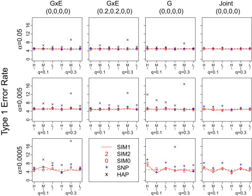
Type I Error Rates of the Proposed Methods

The type I error rates are shown on the scale of 10², 10³, and 10⁴ for nominal level $\alpha =0.05$, 0.005, and 0.0005, respectively. The regions are randomly selected from chromosome 21 to represent six different scenarios listed on the x axis: two levels of disease allele frequencies ($q=0.1$ and 0.3) combined with three levels of LD pattern (high, medium, and low). A high-LD value reflects stronger correlation between the observed markers and the two unobserved risk loci. The panel titles indicate the value of $(\gamma G_1,\gamma G_2,\gamma G{E}_1,\gamma G{E}_2)$, that is the effect sizes of the main genetic effects and gene-environment interactions at the two risk loci used in generating simulated data. Each of the type I error rates is calculated on the basis of 50,000 replications for $\left({\gamma }_{G_1},{\gamma }_{G_2},{\gamma }_{G{E}_1},{\gamma }_{G{E}_2}\right)=\left(0,0,0,0\right)$ and 20,000 replications for $\left(0.2,0.2,0,0\right)$. The type I error rates for HAP-G at $\alpha =0.0005$ are given below as some are beyond the plotting range: (0.00454, 0.00266, 0.0023, 0.00158, 0.00794, and 0.00072).

The power was evaluated for each of the 1734 regions on the basis of 100 replications at the nominal level of 0.0005. The results are shown in Figure 2 (G × E test), Figure 3 (G test), and Figure 4 (joint test). The 1734 regions were grouped into 12 categories, combinations of the four scenarios of allele frequencies and the three LD patterns. The risk allele frequencies from rare to common are categorized as follows: (A) both allele frequencies are less than 0.05, (B) sums of allele frequencies that are less than 0.3 but excluding those in (A), (C) sums of allele frequencies that are between 0.3 and 0.6, and (D) sums of allele frequencies that are greater than 0.6. The clustering of LD patterns is based on the following thresholds: an average $R^2>0.6$ for high, an average $R^2\in \left(0.25,0.6\right)$ for medium, and an average $R^2<0.25$ for low.

Figure 2.

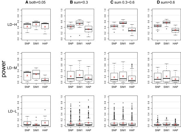
Boxplot of Power of G × E Test from the 1734 Regions on Chromosome 21

The × sign indicates the average power. The power at a region is calculated on the basis of 100 replications at a nominal level of 0.0005. The results are grouped into 12 categories on the basis of frequencies of the risk alleles and LD patterns. The risk allele frequencies from rare to common are categorized as (A) both allele frequencies $<0.05$; (B) sums of allele frequencies $<0.3$ but excluding (A); (C) sums of allele frequencies between 0.3 and 0.6; and (D) sums of allele frequencies $>0.6$. The clustering of LD patterns is done according to the following thresholds: average $R^2>0.6$ for high (LD-H), average $R^2\in \left(0.25,0.6\right)$ for medium (LD-M), and average $R^2<0.25$ for low (LD-L).

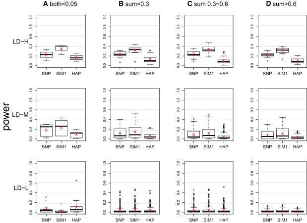
Figure 3.

Boxplot of Power of G Test from the 1734 Regions on Chromosome 21

The × sign indicates the average power. The power at a region is calculated on the basis of 100 replications at a nominal level 0.0005. The results are grouped into 12 categories on the basis of frequencies of the risk alleles and LD patterns. The risk allele frequencies from rare to common are categorized as (A) both allele frequencies $<0.05$; (B) sums of allele frequencies $<0.3$ but excluding (A); (C) sums of allele frequencies between 0.3 and 0.6; and (D) sums of allele frequencies $>0.6$. The clustering of LD patterns is done according to the following thresholds: average $R^2>0.6$ for high (LD-H), average $R^2\in \left(0.25,0.6\right)$ for medium (LD-M), and average $R^2<0.25$ for low (LD-L).

Figure 4.

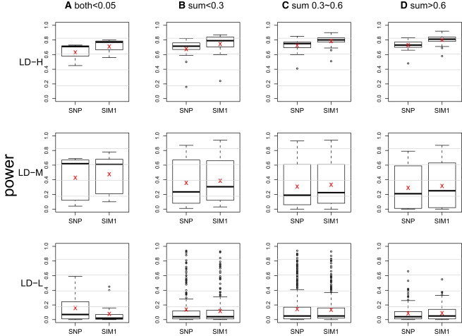
Boxplot of Power of Joint Test from the 1734 Regions on Chromosome 21

The × sign indicates the average power. The power at a region is calculated on the basis of 100 replications at a nominal level 0.0005. The results are grouped into 12 categories on the basis of frequencies of the risk alleles and LD patterns. The risk allele frequencies from rare to common are categorized as (A) both allele frequencies $<0.05$; (B) sums of allele frequencies $<0.3$ but excluding (A); (C) sums of allele frequencies between 0.3 and 0.6; and (D) sums of allele frequencies $>0.6$. The clustering of LD patterns is done according to the following thresholds: average $R^2>0.6$ for high (LD-H), average $R^2\in \left(0.25,0.6\right)$ for medium (LD-M), and average $R^2<0.25$ for low (LD-L).

A similar pattern was observed across Figures 2–4, hence we concentrate on explaining Figure 2. In regions that exhibit low LD (LD-L), all three methods lacked power and had roughly equal performance. The exception is in (A), where the SIM1 method performed worse than the other two. The situation that all three methods had similarly low power is not surprising because LD-L represents regions that contained markers with little information about the two risk loci. The lone exception in LD-L (A) can be explained by the fact that the SIM1 method is best applied in scenarios where a large number of markers have at least medium-level LD with the risk loci, but in LD-L (A), such a scenario only occurred in 13% of the regions. On the other hand, in 60% of the regions, the majority of the markers had no LD with the risk loci, but either one single marker was in perfect LD with one of the risk loci, or two markers were in very high LD with each of the risk loci. The former cases tend to favor the SNP methods, whereas the latter tend to favor the HAP methods (and the remaining 27% were regions where all markers had extremely low LD with the risk loci). In the scenarios of LD-L with (B), (C), and (D), we did not observe such a large proportion of extreme cases, and this resulted in a more comparable performance of the three methods. Finally, compared to regions with LD-L, in the regions with medium LD (LD-M), we observed a uniform increase of power in all three methods, and SIM1 has a slightly greater power. The power gain was more pronounced for high-LD regions (LD-H), where SIM1 showed more power than the other two methods.

To understand the impact of different weighting schemes in the similarity regression, we repeated the same analysis with SIM1, SIM2, and SIM0 (Figure 5). Because the overall patterns were similar across different tests, we present the results from the G × E and G tests. Figure 5 presents the box plots of power for the same regions as shown previously, except that panels (C) and (D) in Figures 2–4 were grouped together to represent common-variant scenarios. We also marked the corresponding average power of SNP (solid line) and HAP (dotted line) for comparison. We observed the following features: (1) SIM0 and SIM2 had very similar power in almost all situations; (2) when risk alleles are common (i.e., [C] and [F]), SIM2 and SIM0 had similar or slightly better power than SIM1, although the difference was not very obvious; and (3) when the risk alleles are uncommon or rare, SIM1 started to gain some traction in improving power. The power improvement became more substantial for rarer alleles. For example, in situations with a moderate LD level, SIM1 had higher power than SNP and HAP, whereas SIM2 and SIM0 did not.

Figure 5.

Boxplot of Power of G × E Test and G Test with Different Weights—SIM1, SIM2, and SIM0—from the 1734 Regions on Chromosome 21

The × sign indicates the average power of the method shown on the x axis. The solid and dotted lines indicate the average power of SNP test and HAP test, respectively. The power at a region is calculated on the basis of 100 replications at a nominal level 0.0005. The results are grouped into nine categories on the basis of frequencies of the risk alleles and LD patterns. The risk allele frequencies from rare to common are categorized: (A and D) both allele frequencies $<0.05$; (B and E) sums of allele frequencies $<0.3$ but excluding (A) and (D); (C and F) sums of allele frequencies $>0.3$. The clustering of LD patterns is done according to the following thresholds: average $R^2>0.6$ for high (LD-H), average $R^2\in \left(0.25,0.6\right)$ for medium (LD-M), and average $R^2<0.25$ for low (LD-L).

Application to Real Data

We applied the similarity regression on samples collected from the VISP trial. VISP was a multicenter, double-blind, randomized, controlled clinical trial that aimed to study the effect of vitamins on preventing recurrent stroke. The VISP trial was conducted under institutional review board approval at the Wake Forest University School of Medicine and at each of the clinic sites and adhered to the tenets of the Declaration of Helsinki. Written informed consent was obtained from all patients participating in the study. The trial enrolled patients who were 35 or older with a nondisabling cerebral infarction [MIM 601367] within 120 days of randomization and Hcy levels in the top quartile for the U.S. population. Subjects were randomly assigned to receive daily doses of either a high-dose formulation (containing 25 mg vitamin B₆, 0.4 mg vitamin B₁₂, and 2.5 mg folic acid) or a low-dose formulation (containing 200 μg vitamin B₆, 6 μg vitamin B₁₂, and 20 μg folic acid). The patients were followed up for a maximum of 2 years, and the average follow-up time was 1.7 years. About 2100 of the VISP participants provided DNA samples, and genotype information was collected from candidate genes selected across the genome that are involved in homocysteine metabolism, stroke risk, and atherosclerosis [MIM 209010]. After quality control, the dataset consists of 1944 subjects and genotypes of 1393 SNPs collected from 215 candidate genes. More details on the VISP trial and VISP genetic study can be found in Toole et al.⁴⁸ and Hsu et al.,⁴⁹ respectively.

Our analysis here focused on the genetic influence on the Hcy level obtained from a 2 hr methionine load test measured at baseline. It has been suggested that Hcy level can be used to predict risk of recurrent stroke and symptomatic coronary heart disease, and genetic variations might be attributed to mild to moderate hyperhomocystinemia [MIM 603174]. Given that the Hcy level tends to increase with age, we also investigated the potential gene-age interaction effects on Hcy. We conducted gene-based analyses; we used the proposed SIM1 method to assess the significant level of each gene and compared it to the available benchmark, SNP, and/or HAP methods. As in the original study,⁴⁹ we adjusted for age, sex, and race in each analysis. The Bonferroni threshold for p value is $0.05/215=2.33\times {10}^{-4}.$

We first used the joint test to perform a gene-based scan to evaluate the gene and gene-age effects on the change in postmethionine load Hcy level (i.e., postmethionine load test Hcy − baseline fasting Hcy). If a gene is rejected by a joint test, the G × E and G tests can be used to further refine the sources of identified signals. The joint test is a suitable screening tool for scenarios in which the underlying gene-age interaction mechanism is little known^32,41 because it assesses the genetic main effect and gene-age interactions simultaneously. The p values of the testing results for each gene (sorted by gene names) are shown in Figure 6. For joint tests, one gene was found to be significant (CBS [MIM 613381]), and both SIM1 and SNP tests yield significant p values. The p value of the SIM1 joint is $2.46\times {10}^{-5}$, and the follow-up analysis reveals that the signal is caused by the genetic main effect instead of gene-age interactions: the p value of SIM G × E is 0.614, and the p value of SIM G is $1.99\times {10}^{-6}$. The SNP joint test has the adjusted minimum p value (adjusted for the 10 typed SNPs in CBS) of $2.06\times {10}^{-5}$. The adjusted minimum p value is obtained by $1-{\left(1-\mathrm{raw}\mathrm{p}\mathrm{value}\right)}^{k_{\text{e}\mathit{f}\mathit{f}}}$ where $k_{\text{e}\mathit{f}\mathit{f}}=7.59$ is the effective number of independent tests estimated with the method of Moskvina and Schmidt⁴⁵ after accounting for the LD in CBS. The adjusted minimum p value for the SNP G × E test is 0.700, and for SNP G test it is $9.42\times {10}^{-6}$. Finally, the HAP G × E test yielded a p value of 0.362, and HAP G test yielded a significant p value of $1.02\times {10}^{-5}$. Variants in CBS have previously been associated with postmethionine load Hcy levels and change in Hcy levels.^49–52 A common 68 bp insertion at the intron 7-exon 8 boundary of CBS and the 31 bp variable number of tandem repeats (VNTR) might be genetic determinants of postmethionine load Hcy levels. Because postmethionine load Hcy levels are found to have an increased risk for cardiovascular disease, CBS could be also considered a risk factor for cardiovascular disease.

Figure 6.

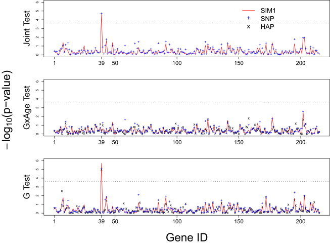
p Values with Negative Log 10 Transformation for the VISP Trial Analysis

The x axis shows the gene IDs sorted by the alphabetic order of the gene names, and gene ID 39 is CBS. The red line indicates results for SIM1, + for SNP method, and × for HAP method. The results for the SNP methods are based on the adjusted minimum p values that adjust for the multiple SNPs in a gene. The adjusted minimum p value is obtained by $1-{\left(1-\text{raw}\mathrm{p}\mathrm{value}\right)}^{k_{eff}}$, where k_eff is the effective number of independent tests estimated with the method of Moskvina and Schmidt⁴⁵ after accounting the LD among SNPs in a gene. A few genes are not plotted on the graph for the HAP methods because of convergence failure at these locations. This failure is mostly attributed to excessive number of SNPs in the gene.

Discussion

Association analyses at the gene, pathway, and exon levels (here by marker-set analysis) hold great promise in evaluating modest etiological effects of genes with data from genome-wide association studies (GWAS) or next-generation sequencing. However, currently available methods tend to target either rare or common variants but not both, assume same-direction effects for loci within a marker set, use a testing framework that cannot accommodate covariates, or do not have the capacity to assess interaction effects. In this article, we propose a flexible, powerful and computationally efficient method to conduct marker-set analysis for assessing gene and gene-environment interactions on quantitative traits. The proposed method is constructed via a similarity regression framework under which we regress trait similarity on genetic similarity. The framework incorporates interaction effects, can adjust for covariates, and is applicable to both observed and imputed dosage genotypes. We develop a series of statistical tests that can be used for genetic marginal main effects, G × E interactions, or the joint effect of the two. We demonstrated that a similarity regression is equivalent to a haplotype random-effects model. The equivalence enabled us to analytically derive the asymptotic distributions of the test statistics and provide a permutation-free procedure to assess significance. The software implementing the proposed methods is available at the authors' website (see Web Resources).

The proposed method uses genetic similarity to aggregate information across markers and integrates adaptive weights dependent on allele frequencies to accommodate common and uncommon variants. Collapsing information at the similarity level instead of the genotype level avoids canceling signals with opposite etiological effects and is applicable to any class of genetic variants without having to dichotomize the allele types. As demonstrated in the simulation, incorporating frequency weights gives the method satisfactory power for detecting both common and uncommon variants. The simulation results also reveal that its performance is sensitive to the signal-to-noise ratio (e.g., LD) among all loci included in the marker-set analysis. The higher the ratio is, the greater the power gain for the proposed methods. As discussed in the next paragraph, it is possible to increase the signal-to-noise ratio to maximize the chance of power gain, such as by using functional, biological or LD information to downweight the contribution from noise markers. In practice, the underlying LD levels are not known and will vary from regions to regions, it is less likely to choose one best performing method in advance. In addition, in GWAS, the low-LD scenario would occur less frequently by design, and in sequencing studies the number of risk loci in a set should be higher than what we considered in the simulation. Given these considerations, the proposed method can serve as a sensible and robust tool for evaluating association of complex traits in whole-genome marker-set analyses.

The inclusion of nonfunctional loci (i.e., nonrisk markers that are not in LD with the risk loci) is a major factor influencing the performance of all marker-set approaches. Intelligently incorporating LD information and biological knowledge into the collapsing process, and downweighting the contribution of nonfunctional markers will be a useful solution. In our framework, biological and functional information, as pioneered and comprehensively reviewed in Price et al.¹⁰ and Schaid³⁸ can be naturally incorporated through the weight matrix, $W_m.$ One unique feature of our weighting framework is that it allows functional weights at the allele-specific level (as opposed to locus-specific level), such as the impact of a specific mutation sequence on protein functions, structures, or stability. We are exploring mechanisms to include genomic knowledge on the basis of functionality, biological pathways, and system biological networks.

One key requirement for the proposed method to have power for both common and uncommon variants is that the similarity level be weighted by allele frequency at order k (i.e., $q^{-k}$). Although the principle is to upweight similarities that are contributed by rare variants, there are no clear rules for what the specific form of the weights should be as a function of the allele frequencies. Kwee et al.²³ considered both $k=1$ and $k=1/2$ when calculating the IBS kernel and concluded that the former might be too strong and the latter is more suitable in their setting. Wu et al.²⁴ therefore used $k=1/2$ in their work. When aggregating information of multiple loci through weighted genotype sum, Madsen and Browning⁸ considered their weights in the order of $k=1/2$ from the binomial standard deviation (SD) viewpoint. Here, we evaluated these different choices of k under our framework (i.e., SIM1 $\left[k=1\right],$ SIM2 $\left[k=1/2\right]$, and SIM0 $\left[k=0\right].$). We found that SIM2 might be too mild and tends to yield similar results as the unweighted SIM0. One main difference between our weighting framework and others is that we assign weights for every allele, whereas others only assign weights for minor alleles. To illustrate the impact of the difference, consider the similarity score between a heterozygous pair. Our weights yield a score of $q_{\text{minor}}^{-1/2}+q_{\text{major}}^{-1/2}$, whereas those weights placed only on minor alleles yield a bigger score of $q_{\text{minor}}^{-1/2}\times 2$ and give a stronger weighting effect.

Simulation results also suggest that larger values of k can greatly boost power for detecting rare variants, but it also risks losing power when the risk variant is common. We focused on SIM1 on the basis of its superior power for rare variants and comparable power for common variants. It is possible that the optimal weights would lie somewhere between $k=1$ and $k=1/2$, and we are investigating further how to identify an optimal order. Alternatively, one can use centered genotype scoring to account for sharing of rarer alleles.⁵³ To center the allele count vector $G_{m,i}$, we define $G_{m,i}^{\ast }=G_{m,i}-{\overline{G}}_m$, where ${\overline{G}}_m$ is the vector of population allele frequency for marker m. Then the similarity score $S_{ij}^{\ast }$ is obtained by $1/M\times {\sum }_{m=1}^M{G}_{m,i}^{\ast T}{G}_{m,j}^{\ast }$. The centering strategy bypasses the need of allele-frequency-dependent weights and hence avoids the choice of an order k. Studies to understand the pros and cons of centering versus weighting strategies are underway.

Appendix A: Expectation-Maximization Algorithm for the REML Estimates of τ and σ When Testing for G × E H₀: ϕ = 0

Let $u=K^{T}Y$ be a set of $n-d$ linearly independent contrasts of Y with $K{K}^T=I-X{\left(X^{T}X\right)}^{-1}{X}^T$ and $K^{T}K=I_{n\text{×}n}$. Then the conditional distribution of u given $\beta ,$ denoted by $f\left(u|\beta \right)$, is normal with mean $K^{T}H\beta$ and variance $\sigma I$ and does not depend on the fixed effect $\gamma .$ Therefore, the REML estimations of τ and σ can be based on its marginal distribution $f\left(u\right)=\int f\left(u|\beta \right)f\left(\beta \right)d\beta .$ This motivated an expectation-maximization algorithm based on observed data u and missing data β. The complete-data log likelihood is given by

$$\begin{array}{l}\log f\left(u,\beta ;\tau ,\sigma \right)=\log f\left(u|\beta ;\tau ,\sigma \right)+\log f\left(\beta ;\tau ,\sigma \right)\hfill \\ =-\frac{n-d}{2}\log \sigma -\frac{1}{2\sigma }{\left(u-K^{T}H\beta \right)}^T\left(u-K^{T}H\beta \right)-\frac{L}{2}\log \tau -\frac{1}{2}\log \left|R\right|-\frac{1}{2\tau }{\beta }^T{R}^{-1}\beta .\end{array}$$

In the expectation step (E-step), we compute $Q\left(\tau ,\sigma ;{\hat{\tau }}^{\left(t\right)},{\hat{\sigma }}^{\left(t\right)}\right)$, the conditional expected value of $\log f\left(u,\beta ;\tau ,\sigma \right)$ given the observed data u assuming $\left(\tau ,\sigma \right)=\left({\hat{\tau }}^{\left(t\right)},{\hat{\sigma }}^{\left(t\right)}\right)$, where ${\hat{\tau }}^{\left(t\right)}$ and ${\hat{\sigma }}^{\left(t\right)}$ are the estimates at the tth iteration.

$$\begin{array}{l}Q\left(\tau ,\sigma ;{\hat{\tau }}^{\left(t\right)},{\hat{\sigma }}^{\left(t\right)}\right)\equiv \text{E}\left[\log f\left(u,\beta ;\tau ,\sigma \right)|u;{\hat{\tau }}^{\left(t\right)},{\hat{\sigma }}^{\left(t\right)}\right]\hfill \\ =-\frac{n-d}{2}\log \sigma -\frac{1}{2\sigma }\text{E}\left[{\left(u-K^{T}H\beta \right)}^T\left(u-K^{T}H\beta \right)|u;{\hat{\tau }}^{\left(t\right)},{\hat{\sigma }}^{\left(t\right)}\right]-\frac{L}{2}\log \tau -\frac{1}{2}\log \left|R\right|-\frac{1}{2\tau }\text{E}\left[{\beta }^T{R}^{-1}\beta |u;{\hat{\tau }}^{\left(t\right)},{\hat{\sigma }}^{\left(t\right)}\right].\hfill \end{array}$$

In the maximization step (M-step), we solve for $\partial Q/\partial \tau =0$ and $\partial Q/\partial \sigma =0$ and obtain

$${\hat{\tau }}^{\left(t+1\right)}=\frac{1}{L}\text{E}\left[{\beta }^T{R}^{-1}\beta |u;{\hat{\tau }}^{\left(t\right)},{\hat{\sigma }}^{\left(t\right)}\right]=\frac{1}{L}\tilde{\beta }{R}^{-1}{\tilde{\beta }}^{-1}+\mathrm{tr}\left(R^{-1}\tilde{W}\right),$$

and

$${\hat{\sigma }}^{\left(t+1\right)}=\frac{1}{n-d}\text{E}\left[{\left(u-K^{T}H\beta \right)}^T\left(u-K^{T}H\beta \right)|u;{\hat{\tau }}^{\left(t\right)},{\hat{\sigma }}^{\left(t\right)}\right]={\left(Y-H\tilde{\beta }\right)}^{T}A\left(Y-H\tilde{\beta }\right)+\mathrm{tr}\left(H^{T}AH\tilde{W}\right).$$

In the above equations, $A=K{K}^T=I-X{\left(X^{T}X\right)}^{-1}{X}^T$, $\tilde{\beta }\equiv \mathrm{E}\left(\beta |u;;{\hat{\tau }}^{\left(t\right)},{\hat{\sigma }}^{\left(t\right)}\right)=\tau R{H}^T{P}_{1}Y,$ and $\tilde{W}\equiv \mathrm{var}\left(\beta |u;{\hat{\tau }}^{\left(t\right)},{\hat{\sigma }}^{\left(t\right)}\right)=\tau R-{\tau }^{2}R{H}^{T}PHR$. The conditional moments of β given u are obtained directly from the normality of the joint distribution of $\left(u,\beta \right).$ The calculation of the project matrix P₁ requires inverting the $n\times n$ nonsparse matrix $V_1,$ which can be computational burdensome. To speed up the computation, we rewrite

$$V_1=\tau S+\sigma I=\sigma \left\{I+\frac{\tau }{\sigma }S\right\}=\sigma \left\{I+\frac{\tau }{\sigma }E\text{Λ}{E}^T\right\},$$

where $S=E\text{Λ}{E}^T$, the eigenvalue decomposition of matrix S. Then by the fact that ${\left(I+B_1{B}_2\right)}^{-1}=I-B_1{\left(I+B_2{B}_1\right)}^{-1}{B}_2$, we can rewrite $V_1^{-1}=1/\sigma \left\{I-\tau /\sigma E\text{Λ}{\left[I+E^T\tau /\sigma E\text{Λ}\right]}^{-1}{E}^T\right\}=1/\sigma \left\{I-\tau E\text{Λ}{\left[\sigma I+\tau E^{T}E\text{Λ}\right]}^{-1}{E}^T\right\},$ in which the calculation involves only an inversion of an $L\times L$ matrix.

Appendix B: Derivation of the Score Test Statistics and Their Asymptotic Distribution

For quantitative traits that follow a normal distribution directly or after appropriate transformations, model (Equation 2) reduces to the following linear mixed model (LMM) in matrix notation

$$\mathbf{Y}=\mathbf{1}{\gamma }_0+X\gamma +H\beta +DH\lambda +\epsilon ,\text{with}\beta \sim \text{N}\left(0,\tau R\right),\lambda \sim \text{N}\left(0,\varphi R\right),\text{and}\epsilon \sim \text{N}\left(0,\sigma I\right)$$ (Equation 4)

where $Y^T=\left[Y_1,\cdots ,Y_n\right],$ 1 is an $n\times 1$ vector of 1s, $X^T=\left[X_1,\cdots ,X_n\right],$$D=diag\left\{X_i\right\}$, and ${\epsilon }_{n\text{×}1}^T=\left[e_1,\cdots ,e_n\right].$ Because our primary interest is to test the variance components ϕ and τ, we consider the restricted maximum likelihood (REML) log-likelihood function of variance components $\left(\tau ,\varphi ,\sigma \right):$${\ell }_{REML}\left(\tau ,\varphi ;Y\right)=-\left\{\log \left|V\right|+\log \left|X^T{V}^{-1}X\right|+Y^{T}PY\right\}/2,$ where V is the marginal variance of Y and $V=\varphi \text{Σ}+\tau S+\sigma I$, where $S=HR{H}^T$ and $\text{Σ}=DSD$; $P=V^{-1}-V^{-1}X{\left(X^T{V}^{-1}X\right)}^{-1}{X}^T{V}^{-1}$ is the projection matrix for the LMM (4).

Let $U_{\varphi }\left(\varphi ,\tau ,\sigma \right)$ and $U_{\tau }\left(\varphi ,\tau ,\sigma \right)$ denote the score functions based on the REML function for ϕ and $\tau ,$ respectively. Simple algebra⁵⁴ shows that under $H_0:\varphi =0,$

$$U_{\varphi }\left(0,\hat{\tau },\hat{\sigma }\right)={\frac{\partial {\ell }_{REML}\left(\tau ,\varphi ,\sigma \right)}{\partial \varphi }|}_{\varphi =0,\tau =\hat{\tau },\sigma =\hat{\sigma }}=\frac{1}{2}\left\{Y^T{P}_1\text{Σ}{P}_{1}Y-\mathrm{tr}\left(P_1\text{Σ}\right)\right\},$$ (Equation 5)

and under $H_0:\tau =0$ (and with the constrain of $\varphi =0$),

$$U_{\tau }\left(0,0,\hat{\sigma }\right)={\frac{\partial {\ell }_{REML}\left(\tau ,\varphi ,\sigma \right)}{\partial \tau }|}_{\varphi =0,\tau =0,\sigma =\tilde{\sigma }}=\frac{1}{2}\left\{Y^T{P}_{0}S{P}_{0}Y-\mathrm{tr}\left(P_{0}S\right)\right\}.$$ (Equation 6)

In the above equations, $\left(\tilde{\tau },\tilde{\sigma }\right)$ are the REML estimates of $\left(\tau ,\sigma \right)$ under $H_0:\varphi =0$ as given in Appendix A, and $\tilde{\sigma }$ the REML estimate of σ when $\tau =\varphi =0$. Recall that $P_t=V_t^{-1}-V_t^{-1}X{\left(X^T{V}_t^{-1}X\right)}^{-1}{X}^T{V}_t^{-1}$ where $t\in \left\{0,1\right\},$ and $V_1=\tau S+\sigma I$ and $V_0=\sigma I$.

Null Distribution of the Score Statistics for G × E Test and G Test

As shown in Tzeng and Zhang,²² the score statistics under H₀ are not asymptotically normal because the design matrix H for the random effects β is not block diagonal and the dimension of β is fixed. We thus use the first terms of the score statistics as the testing statistics and obtain $T_{G\text{×}E}=Y^T{P}_1\text{Σ}{P}_{1}Y/2$ and $T_G=Y^T{P}_{0}S{P}_{0}Y/2.$ Below we derive the asymptotic null distribution of $T_{G\text{×}E},$ and similar steps can be used to obtain the distribution for $T_G.$ If $\mu =\mathbf{1}{\gamma }_0-X\gamma ,$ and $\mathbf{Z}=V_1^{-1/2}\left(\mathbf{Y}-\mu \right)$, then Z follows a standard multivariate normal distribution. We rewrite $T_{G\text{×}E}={\mathbf{Z}}^T\left(1/2V_1^{1/2}{P}_1\text{Σ}{P}_1{V}_1^{1/2}\right)\mathbf{Z}\equiv {\mathbf{Z}}^T{C}_{G\text{×}E}\mathbf{Z}$, which is true because ${\mu }^T{P}_1=0$ by the fact of P₁ being a projection matrix. Define e_i and ${\eta }_i$, the eigenvector and eigenvalue of matrix $C_{G\text{×}E}$, respectively. Then $T_{G\text{×}E}={\sum }_{i=1}^c{\eta }_i{\left(e_i^{T}Z\right)}^2\equiv {\sum }_{i=1}^L{\eta }_i{\tilde{Z}}_i^2,$ with ${\tilde{Z}}_i^2$ follows a 1 degree-of-freedom chi-square distribution. In reality, $\left(\tau ,\sigma \right)$ is evaluated at their restricted maximum likelihood estimates $\left(\hat{\tau },\hat{\sigma }\right)$. Following Tzeng and Zhang,²² the distribution of $T_{G\times E}$ can be approximated by the distribution of ${\sum }_{i=1}^c{\hat{\eta }}_i{\chi }_{i1}^2$, where ${\hat{\eta }}_i$'s are the nonzero eigenvalues of matrix ${C_{G\times E}|}_{\tau =\hat{\tau },\sigma =\hat{\sigma }}$. The distribution of $T_{G\text{×}E}$ can be approximated by the three-moment approximation method of.⁴³ The level- α significance threshold is estimated by ${\kappa }_1+\left({\chi }_{\alpha }-h^{\prime }\right)\times \sqrt{{\kappa }_2/h^{\prime }}$, where ${\kappa }_j={\sum }_i{\eta }_i^j,$$h^{\prime }={\kappa }_2^3/{\kappa }_3^2$ and ${\chi }_{\alpha }$ is the α th quantile of ${\chi }_{h^{\prime }}^2$ (i.e., chi-square distribution with $h^{\prime }$ degrees of freedom). Alternatively, one can report the p value of the observed statistic $T_{G\text{×}E}$ by $P<{\chi }_{h^{\prime }}^2>{\chi }^{\ast }$, where ${\chi }^{\ast }=\left(T_{G\text{×}E}-{\kappa }_1\right)\times \sqrt{h^{\prime }/{\kappa }_2}+h^{\prime }$.

By the same manner, the distribution of T_G can also be approximated by the three-moment approximation as above, except that the eigenvalues η_is are obtained from matrix $C_G={1/2V_0^{1/2}{P}_{0}S{P}_0{V}_0^{1/2}|}_{\sigma =\tilde{\sigma }}$.

Null Distribution of the Score Statistics for Joint Test

The test statistic for the joint hypothesis $H_0:\varphi =\tau =0$ is $T_{\text{joint}}=T_G+T_{G\times E}^{\left(0\right)}$, where T_G is defined as before and $T_{G\text{×}E}^{\left(0\right)}=1/2Y^T{P}_0\sum P_{0}Y$, i.e., $T_{G\text{×}E}$ evaluated at $\varphi =\tau =0$ and $\sigma =\tilde{\sigma }.$ A direct (unweighted) sum is used here because X has been prestandardized to mean = 0 and variance = 1, and hence T_G and $T_{G\text{×}E}$ are on the same scale. We found that the performance of the unweighted sum is very similar to that of the weighted sum, $T_{joint}^{wt}=w_G\times T_G+w_{G\text{×}E}\times T_{G\text{×}E}^{\left(0\right)}$, where the weights $w_i=E\left(T_i\right)/var\left(T_i\right)$. By a similar derivation as in the G × E test, it can be shown that the null distribution of $T_{joint}$ also has a weighted chi-square distribution and can be approximated by the three-moment approximation. The procedure is the same as what mentioned for the G × E test, except that the eigenvalues should be obtained from the matrix $C_{joint}={1/2V_0^{1/2}{P}_0\left(S+\text{Σ}\right)P_0{V}_0^{1/2}|}_{\sigma =\tilde{\sigma }}$.

Web Resources

The URLs for data presented herein are as follows:

• Jung-Ying Tzeng, http://www4.stat.ncsu.edu/∼tzeng/software.php

• Online Mendelian Inheritance in Man (OMIM), http://www.omim.org

References

- 1.De la Cruz O., Wen X., Ke B., Song M., Nicolae D.L. Gene, region and pathway level analyses in whole-genome studies. Genet. Epidemiol. 2010;34:222–231. doi: 10.1002/gepi.20452. [DOI] [PMC free article] [PubMed] [Google Scholar]
- 2.Fisher R.A. Oliver and Boyd; London: 1932. Statistical methods for research workers. [Google Scholar]
- 3.Li M., Wang K., Grant S.F., Hakonarson H., Li C. ATOM: a powerful gene-based association test by combining optimally weighted markers. Bioinformatics. 2009;25:497–503. doi: 10.1093/bioinformatics/btn641. [DOI] [PMC free article] [PubMed] [Google Scholar]
- 4.Wang T., Elston R.C. Improved power by use of a weighted score test for linkage disequilibrium mapping. Am. J. Hum. Genet. 2007;80:353–360. doi: 10.1086/511312. [DOI] [PMC free article] [PubMed] [Google Scholar]
- 5.Gauderman W.J., Murcray C., Gilliland F., Conti D.V. Testing association between disease and multiple SNPs in a candidate gene. Genet. Epidemiol. 2007;31:383–395. doi: 10.1002/gepi.20219. [DOI] [PubMed] [Google Scholar]
- 6.Wang K., Abbott D. A principal components regression approach to multilocus genetic association studies. Genet. Epidemiol. 2008;32:108–118. doi: 10.1002/gepi.20266. [DOI] [PubMed] [Google Scholar]
- 7.Li B., Leal S.M. Methods for detecting associations with rare variants for common diseases: application to analysis of sequence data. Am. J. Hum. Genet. 2008;83:311–321. doi: 10.1016/j.ajhg.2008.06.024. [DOI] [PMC free article] [PubMed] [Google Scholar]
- 8.Madsen B.E., Browning S.R. A groupwise association test for rare mutations using a weighted sum statistic. PLoS Genet. 2009;5:e1000384. doi: 10.1371/journal.pgen.1000384. [DOI] [PMC free article] [PubMed] [Google Scholar]
- 9.Morgenthaler S., Thilly W.G. A strategy to discover genes that carry multi-allelic or mono-allelic risk for common diseases: a cohort allelic sums test (CAST) Mutat. Res. 2007;615:28–56. doi: 10.1016/j.mrfmmm.2006.09.003. [DOI] [PubMed] [Google Scholar]
- 10.Price A.L., Kryukov G.V., de Bakker P.I., Purcell S.M., Staples J., Wei L.J., Sunyaev S.R. Pooled association tests for rare variants in exon-resequencing studies. Am. J. Hum. Genet. 2010;86:832–838. doi: 10.1016/j.ajhg.2010.04.005. [DOI] [PMC free article] [PubMed] [Google Scholar]
- 11.Tzeng J.Y., Byerley W., Devlin B., Roeder K., Wasserman L. Outlier detection and false discovery rates for whole-genome DNA matching. J. Am. Stat. Assoc. 2003;98:236–246. [Google Scholar]
- 12.Tzeng J.Y., Devlin B., Wasserman L., Roeder K. On the identification of disease mutations by the analysis of haplotype similarity and goodness of fit. Am. J. Hum. Genet. 2003;72:891–902. doi: 10.1086/373881. [DOI] [PMC free article] [PubMed] [Google Scholar]
- 13.Schaid D.J., McDonnell S.K., Hebbring S.J., Cunningham J.M., Thibodeau S.N. Nonparametric tests of association of multiple genes with human disease. Am. J. Hum. Genet. 2005;76:780–793. doi: 10.1086/429838. [DOI] [PMC free article] [PubMed] [Google Scholar]
- 14.Beckmann L., Thomas D.C., Fischer C., Chang-Claude J. Haplotype sharing analysis using mantel statistics. Hum. Hered. 2005;59:67–78. doi: 10.1159/000085221. [DOI] [PubMed] [Google Scholar]
- 15.Wessel J., Schork N.J. Generalized genomic distance-based regression methodology for multilocus association analysis. Am. J. Hum. Genet. 2006;79:792–806. doi: 10.1086/508346. [DOI] [PMC free article] [PubMed] [Google Scholar]
- 16.Dempfle A., Hein R., Beckmann L., Scherag A., Nguyen T.T., Schäfer H., Chang-Claude J. Comparison of the power of haplotype-based versus single- and multilocus association methods for gene x environment (gene x sex) interactions and application to gene x smoking and gene x sex interactions in rheumatoid arthritis. BMC Proc. 2007;1(Suppl 1):S73. doi: 10.1186/1753-6561-1-s1-s73. [DOI] [PMC free article] [PubMed] [Google Scholar]
- 17.Tzeng J.Y., Zhang D., Chang S.M., Thomas D.C., Davidian M. Gene-trait similarity regression for multimarker-based association analysis. Biometrics. 2009;65:822–832. doi: 10.1111/j.1541-0420.2008.01176.x. [DOI] [PMC free article] [PubMed] [Google Scholar]
- 18.Mukhopadhyay I., Feingold E., Weeks D.E., Thalamuthu A. Association tests using kernel-based measures of multi-locus genotype similarity between individuals. Genet. Epidemiol. 2010;34:213–221. doi: 10.1002/gepi.20451. [DOI] [PMC free article] [PubMed] [Google Scholar]
- 19.Wei Z., Li M., Rebbeck T., Li H. U-statistics-based tests for multiple genes in genetic association studies. Ann. Hum. Genet. 2008;72:821–833. doi: 10.1111/j.1469-1809.2008.00473.x. [DOI] [PMC free article] [PubMed] [Google Scholar]
- 20.Goeman J.J., van de Geer S.A., de Kort F., van Houwelingen H.C. A global test for groups of genes: testing association with a clinical outcome. Bioinformatics. 2004;20:93–99. doi: 10.1093/bioinformatics/btg382. [DOI] [PubMed] [Google Scholar]
- 21.Goeman J.J., van de Geer S.A., van Houwelingen H.C. Testing against a high dimensional alternative. J. R. Stat. Soc. Series B Stat. Methodol. 2005;68:477–493. [Google Scholar]
- 22.Tzeng J.Y., Zhang D. Haplotype-based association analysis via variance-components score test. Am. J. Hum. Genet. 2007;81:927–938. doi: 10.1086/521558. [DOI] [PMC free article] [PubMed] [Google Scholar]
- 23.Kwee L.C., Liu D., Lin X., Ghosh D., Epstein M.P. A powerful and flexible multilocus association test for quantitative traits. Am. J. Hum. Genet. 2008;82:386–397. doi: 10.1016/j.ajhg.2007.10.010. [DOI] [PMC free article] [PubMed] [Google Scholar]
- 24.Wu M.C., Kraft P., Epstein M.P., Taylor D.M., Chanock S.J., Hunter D.J., Lin X. Powerful SNP-set analysis for case-control genome-wide association studies. Am. J. Hum. Genet. 2010;86:929–942. doi: 10.1016/j.ajhg.2010.05.002. [DOI] [PMC free article] [PubMed] [Google Scholar]
- 25.Schaid D.J. Genomic similarity and kernel methods I: advancements by building on mathematical and statistical foundations. Hum. Hered. 2010;70:109–131. doi: 10.1159/000312641. [DOI] [PMC free article] [PubMed] [Google Scholar]
- 26.Neale B.M., Rivas M.A., Voight B.F., Altshuler D., Devlin B., Orho-Melander M., Kathiresan S., Purcell S.M., Roeder K., Daly M.J. Testing for an unusual distribution of rare variants. PLoS Genet. 2011;7:e1001322. doi: 10.1371/journal.pgen.1001322. [DOI] [PMC free article] [PubMed] [Google Scholar]
- 27.Luan Y., Li H. Group additive regression models for genomic data analysis. Biostatistics. 2008;9:100–113. doi: 10.1093/biostatistics/kxm015. [DOI] [PubMed] [Google Scholar]
- 28.Chatterjee N., Kalaylioglu Z., Moslehi R., Peters U., Wacholder S. Powerful multilocus tests of genetic association in the presence of gene-gene and gene-environment interactions. Am. J. Hum. Genet. 2006;79:1002–1016. doi: 10.1086/509704. [DOI] [PMC free article] [PubMed] [Google Scholar]
- 29.Zhao J., Boerwinkle E., Xiong M. An entropy-based statistic for genomewide association studies. Am. J. Hum. Genet. 2005;77:27–40. doi: 10.1086/431243. [DOI] [PMC free article] [PubMed] [Google Scholar]
- 30.Dempfle A., Scherag A., Hein R., Beckmann L., Chang-Claude J., Schäfer H. Gene-environment interactions for complex traits: definitions, methodological requirements and challenges. Eur. J. Hum. Genet. 2008;16:1164–1172. doi: 10.1038/ejhg.2008.106. [DOI] [PubMed] [Google Scholar]
- 31.Thomas D. Gene—environment-wide association studies: emerging approaches. Nat. Rev. Genet. 2010;11:259–272. doi: 10.1038/nrg2764. [DOI] [PMC free article] [PubMed] [Google Scholar]
- 32.Lindström S., Yen Y.C., Spiegelman D., Kraft P. The impact of gene-environment dependence and misclassification in genetic association studies incorporating gene-environment interactions. Hum. Hered. 2009;68:171–181. doi: 10.1159/000224637. [DOI] [PMC free article] [PubMed] [Google Scholar]
- 33.Smith P.G., Day N.E. The design of case-control studies: the influence of confounding and interaction effects. Int. J. Epidemiol. 1984;13:356–365. doi: 10.1093/ije/13.3.356. [DOI] [PubMed] [Google Scholar]
- 34.Thomas D. Methods for investigating gene-environment interactions in candidate pathway and genome-wide association studies. Annu. Rev. Public Health. 2010;31:21–36. doi: 10.1146/annurev.publhealth.012809.103619. [DOI] [PMC free article] [PubMed] [Google Scholar]
- 35.Ballard D.H., Cho J., Zhao H. Comparisons of multi-marker association methods to detect association between a candidate region and disease. Genet. Epidemiol. 2010;34:201–212. doi: 10.1002/gepi.20448. [DOI] [PMC free article] [PubMed] [Google Scholar]
- 36.Chapman J., Whittaker J. Analysis of multiple SNPs in a candidate gene or region. Genet. Epidemiol. 2008;32:560–566. doi: 10.1002/gepi.20330. [DOI] [PMC free article] [PubMed] [Google Scholar]
- 37.Fridley B.L., Jenkins G.D., Biernacka J.M. Self-contained gene-set analysis of expression data: an evaluation of existing and novel methods. PLoS ONE. 2010;5:e12693. doi: 10.1371/journal.pone.0012693. [DOI] [PMC free article] [PubMed] [Google Scholar]
- 38.Schaid D.J. Genomic similarity and kernel methods II: methods for genomic information. Hum. Hered. 2010;70:132–140. doi: 10.1159/000312643. [DOI] [PMC free article] [PubMed] [Google Scholar]
- 39.Cordell H.J. Epistasis: what it means, what it doesn't mean, and statistical methods to detect it in humans. Hum. Mol. Genet. 2002;11:2463–2468. doi: 10.1093/hmg/11.20.2463. [DOI] [PubMed] [Google Scholar]
- 40.Hirschhorn J.N., Daly M.J. Genome-wide association studies for common diseases and complex traits. Nat. Rev. Genet. 2005;6:95–108. doi: 10.1038/nrg1521. [DOI] [PubMed] [Google Scholar]
- 41.Kraft P., Yen Y.C., Stram D.O., Morrison J., Gauderman W.J. Exploiting gene-environment interaction to detect genetic associations. Hum. Hered. 2007;63:111–119. doi: 10.1159/000099183. [DOI] [PubMed] [Google Scholar]
- 42.Zhang D., Lin X. Hypothesis testing in semiparametric additive mixed models. Biostatistics. 2003;4:57–74. doi: 10.1093/biostatistics/4.1.57. [DOI] [PubMed] [Google Scholar]
- 43.Pearson E.S. Note on an approximation to the distribution of non-central χ2. Biometrika. 1959;46:364. [Google Scholar]
- 44.Imhof J.P. Computing the Distribution of Quadratic Forms in Normal Variables. Biometrika. 1961;48:419–426. [Google Scholar]
- 45.Moskvina V., Schmidt K.M. On multiple-testing correction in genome-wide association studies. Genet. Epidemiol. 2008;32:567–573. doi: 10.1002/gepi.20331. [DOI] [PubMed] [Google Scholar]
- 46.Lake S.L., Lyon H., Tantisira K., Silverman E.K., Weiss S.T., Laird N.M., Schaid D.J. Estimation and tests of haplotype-environment interaction when linkage phase is ambiguous. Hum. Hered. 2003;55:56–65. doi: 10.1159/000071811. [DOI] [PubMed] [Google Scholar]
- 47.Schaid D.J., Rowland C.M., Tines D.E., Jacobson R.M., Poland G.A. Score tests for association between traits and haplotypes when linkage phase is ambiguous. Am. J. Hum. Genet. 2002;70:425–434. doi: 10.1086/338688. [DOI] [PMC free article] [PubMed] [Google Scholar]
- 48.Toole J.F., Malinow M.R., Chambless L.E., Spence J.D., Pettigrew L.C., Howard V.J., Sides E.G., Wang C.H., Stampfer M. Lowering homocysteine in patients with ischemic stroke to prevent recurrent stroke, myocardial infarction, and death: the Vitamin Intervention for Stroke Prevention (VISP) randomized controlled trial. JAMA. 2004;291:565–575. doi: 10.1001/jama.291.5.565. [DOI] [PubMed] [Google Scholar]
- 49.Hsu F.C., Sides E.G., Mychaleckyj J.C., Worrall B.B., Elias G.A., Liu Y., Chen W.M., Coull B.M., Toole J.F., Rich S.S. A Transcobalamin 2 gene variant associated with post-stroke homocysteine modifies recurrent stroke risk. Neurology. 2011 doi: 10.1212/WNL.0b013e318233b1f9. in press. [DOI] [PMC free article] [PubMed] [Google Scholar]
- 50.Tsai M.Y., Yang F., Bignell M., Aras O., Hanson N.Q. Relation between plasma homocysteine concentration, the 844ins68 variant of the cystathionine beta-synthase gene, and pyridoxal-5′-phosphate concentration. Mol. Genet. Metab. 1999;67:352–356. doi: 10.1006/mgme.1999.2874. [DOI] [PubMed] [Google Scholar]
- 51.Lievers K.J., Kluijtmans L.A., Heil S.G., Boers G.H., Verhoef P., van Oppenraay-Emmerzaal D., den Heijer M., Trijbels F.J., Blom H.J. A 31 bp VNTR in the cystathionine beta-synthase (CBS) gene is associated with reduced CBS activity and elevated post-load homocysteine levels. Eur. J. Hum. Genet. 2001;9:583–589. doi: 10.1038/sj.ejhg.5200679. [DOI] [PubMed] [Google Scholar]
- 52.Lievers K.J., Kluijtmans L.A., Blom H.J., Wilson P.W., Selhub J., Ordovas J.M. Association of a 31 bp VNTR in the CBS gene with postload homocysteine concentrations in the Framingham Offspring Study. Eur. J. Hum. Genet. 2006;14:1125–1129. doi: 10.1038/sj.ejhg.5201677. [DOI] [PubMed] [Google Scholar]
- 53.Qian D., Thomas D.C. Genome scan of complex traits by haplotype sharing correlation. Genet. Epidemiol. 2001;21(Suppl 1):S582–S587. doi: 10.1002/gepi.2001.21.s1.s582. [DOI] [PubMed] [Google Scholar]
- 54.Harville D.A. Maximum likelihood approaches to variance component estimation and related problems. J. Am. Stat. Assoc. 1977;72:320–338. [Google Scholar]