A Practical Acceleration Algorithm for Real-Time Imaging

Abstract

A practical acceleration algorithm for real-time MRI is presented. Neither separate training scans nor embedded training samples are used. The Kalman filter based algorithm provides a fast and causal reconstruction of dynamic MRI acquisitions with arbitrary readout trajectories. The algorithm is tested against abrupt changes in the imaging conditions and offline reconstructions of in-vivo cardiac MRI experiments are presented.

1 Introduction

Dynamic MRI is an important tool to monitor changes in tissue structure over time. The basic dynamic imaging experiment puts the MRI scanner in a continuous scan mode and the same imaging sequence is repeated periodically to obtain a time series of images. Many dynamic MRI applications reconstruct the images after the data is collected. Real-time MRI has the additional requirement that the reconstruction be performed at the time of the experiment with minimum latency. Along with this reconstruction budget requirement, real-time experiments often explore the advantages of changing the imaging sequence on-the-fly. This capability can decrease the overall scan time and increase the throughput of clinical MRI. Perhaps more importantly, applications such as image-guided therapy and catheter tracking exist as a consequence of real-time imaging.

The main problem of dynamic MRI has been to provide a satisfactory temporal resolution without compromising spatial specifications such as field of view (FOV) and resolution. Since the speed of data acquisition is fundamentally limited by both physical and physiological constraints, accelerated reconstruction techniques have become increasingly popular [1–10]. Naturally, the same problems carry over to real-time imaging. In addition, the acceleration algorithm must be fast and causal. These extra restrictions prevent modern techniques from being applied to real-time imaging. Indeed, many approaches are targeted towards offline reconstruction and assessment. Some of these methods are not causal, while others may require separate initialization scans. Other obstacles include time-consuming reconstruction algorithms and their inability to handle arbitrary readout trajectories. As a result, the sliding window reconstruction is used ubiquitously in clinical real-time applications despite its shortcomings.

The sliding window algorithm convolves the data with a rectangular temporal window. The width of the window is chosen so as to satisfy the spatial Nyquist rate. Thus, the samples within the window receive equal weights. This technique is suitable for arbitrary trajectories, but the temporal blur due to convolution can be intolerable at times. This blur can be decreased by exploiting the temporal redundancy in high frame rate reconstructions, either explicitly or implicitly. For instance, sparse MRI [8] uses the sparsity in the temporal frequency dimension and k-t BLAST [5] exploits the fact that many image pixels are relatively stable while a few pixels display rapid variations. The phenomenon exploited by both of these methods is the same although the approaches are quite different. Recently, the authors proposed a Kalman filter based algorithm that exploits the same redundancy with a fast and causal reconstruction. The results suggest improvements over the sliding window algorithm [11]. However, the algorithm relies on an initialization scan, which nullifies some important advantages of the real-time imaging paradigm.

In this paper, we modify the Kalman algorithm with a real-time imaging focus. The modified algorithm provides fast and causal reconstructions with arbitrary trajectories and it does not use separate training scans. This auto-calibrating algorithm quickly adapts to changing imaging parameters and the reconstruction quality improves over the sliding window reconstruction. Temporal blurring is reduced and anatomical details are better depicted in individual images. As mentioned above, there are already a few robust methods outperforming the sliding window algorithm in an offline reconstruction scenario with a bigger time budget. However, these methods are not real-time capable. Therefore we compare our results to those of the sliding window algorithm. The proposed algorithm benefits from the fact that non-Cartesian trajectories result in incoherent aliasing patterns. Moreover, non-Cartesian trajectories generally have better motion and flow properties [12]. Therefore, the algorithm should perform better with such readout trajectories although there is no difference in the computational steps. Our results were obtained using spiral readouts and we will be implicitly referring to a non-Cartesian trajectory throughout the paper.

The proposed algorithm maintains a dynamic buffer to adapt to changing imaging conditions. The algorithm naturally handles changes in the excitation and acquisition sequences, coil sensitivities and coil noise variances, as well as patient position. A similar idea was applied to k-t BLAST [13], where a short-time Fourier transform was used so as not to wait until the end of the experiment. However, the method was ultimately limited by noncausality, resulting in long latencies.

In the next section, we modify the original Kalman reconstruction algorithm. Section 3 explains the experiments reported in this paper. Results of the in-vivo experiments are given in Section 4. Section 5 concludes with a discussion of the method. In the Appendix, we provide a few implementation details.

Throughout the paper, â represents an estimate of the generic parameter a, var(a) denotes the covariance of a, a^H denotes the Hermitian conjugate of a, and |a| denotes the elementwise absolute value of a. Lastly, in arithmetic operations, × and ÷ denote elementwise multiplication and division, respectively.

2 Theory

2.1 The Kalman filter approximation

An acceleration method based on the Kalman filter was introduced in [11]. The method provides fast and causal reconstructions although it relies on initialization scans. Here, we first summarize that algorithm. Then, the ability of the algorithm to rapidly adapt to changes is shown under steady state conditions and an auto-calibration scheme that does not require extra k-space samples is presented.

A model of multi-coil dynamic MRI experiments with arbitrary readouts is

$$\begin{array}{l}{s}_{t+1}=s_t+u_t\\ x_t=H_t{s}_t+w_t,\end{array}$$ (1)

where s_t is an m² × 1 vector denoting the true noise-free m × m image arranged into a one-dimensional vector, u_t denotes the corresponding difference vector between consecutive true images, x_t denotes the n × 1 vector of actual scanner data, and w_t denotes the corresponding acquisition noise, all at time t. H_t is called the observation matrix and it includes terms due to gridding, Fourier transformation, and coil sensitivities. For a general reference on the Kalman filter, the reader may refer to [15]. The claimed acceleration in our reconstructions is achieved by estimating a full image (ŝ_t) from individual interleaves (x_t) in multi-shot acquisitions, in which case n is significantly smaller than m².

The first line in Eq. 1 puts the modeling burden on u_t. Note that no a priori knowledge is assumed for motion. Therefore, the fate of the reconstruction depends on characterizing the second moment of the difference process, {u_t}. This also provides the algorithm a significant flexibility to operate under changing conditions. The second line in Eq. 1 describes the physical process of data acquisition together with an additive acquisition noise component.

Let ${\overline{Z}}_t=H_t^H{R}_t^{-1}{H}_t$, where R_t = var(w_t) is the acquisition noise covariance matrix allowing different noise variances for individual receive channels. Coil noise cross-correlations are ignored, which are usually small [12]. Let ρ = diag(R_t) denote the vector of noise variances of individual samples. {u_t} is known as the system noise process and we will call the diagonals of its covariance Q_t = cov(u_t) the motion map. P_t denotes the estimation error covariance cov(s_t − ŝ_t). For consistency, we note that we use a simplified notation in this paper and P_t corresponds to P_t,t in Ref. [11].

We assume that Q_t, R_t, Z̄_t and P_t are diagonal. The underlying reasons and theoretical analyses are given in [11]. Also, Ref. [16] suggests tracking the wavelet transform of the underlying image to further improve the diagonal approximation. The diagonal entries of these diagonal matrices are read into m × m images and the most time consuming steps of the general Kalman filter simplify to elementwise calculations. We also have ${\overline{Z}}_t=(n/m^2){\sum }_{i=1}^c{\sigma }_i^{-2}\mid C_i\mid \times \mid C_i\mid$, where C_i denotes the sensitivity map of the i^th coil. Thus, the basic algorithm is given as

$$\begin{array}{l}{P}_0\leftarrow 0,{\widehat{s}}_0=E(s_0)\\ P_t\leftarrow P_{t-1}+Q_{t-1}\\ P_t\leftarrow P_t÷(\mathbf{1}+P_t\times {\overline{Z}}_t)\\ {\widehat{s}}_t\leftarrow {\widehat{s}}_{t-1}+P_t\times [H_t^H((x_t-H_t{\widehat{s}}_{t-1})÷\rho )].\end{array}$$ (2)

Some of the samples from the already oversampled, high SNR, slew-limited central part of k-space are discarded to arrive at approximately uniform sampling densities along a single readout interleaf. This allows for the approximation leading to the fast reconstruction algorithm in Eq. 2, at a small SNR penalty. Moreover, the corresponding SNR loss can be eliminated by first resampling uniformly along the trajectory. Details on initializing the algorithm can be found in [11]. When multiple acquisition channels are used, the data can be combined to be reconstructed together using explicit sensitivity information (SENSE-like [17]) or individual channel data can be reconstructed independently to be combined later (GRAPPA-like [18]). For details, see [11]. In this paper, we employ the combine-then-reconstruct approach.

2.2 Exponentially Fast Reorganization

The algorithm puts exponentially diminishing importance on past data. This property allows the filter to reorganize itself quickly when a (cyclic) steady state is perturbed, either by changing the imaging parameters or by patient motion. The sliding window reconstruction puts equal importance on a finite number of time points. Moreover, it treats every pixel in the same manner. In contrast, the Kalman filter based algorithm uses a pixel-dependent update scheme. All of the available data is utilized, but only the most recent few time points contribute significantly. To see this, define ${\stackrel{\sim }{s}}_t=P_t{H}_t^H{R}_t^{-1}{x}_t$, t ≥ 1 and s̃₀ = s₀ so that for t ≥ 1, s̃_t denotes aliased contributions of individual observations. The diagonal matrices P_t serve as image masks suppressing some of the aliased energy. Moreover, let

$${\mathrm{\Gamma }}_{t,t^{\prime }}=(I-P_t{H}_t^H{R}_t^{-1}{H}_t)\dots (I-P_{t^{\prime }+1}{H}_{t^{\prime }+1}^H{R}_{t^{\prime }+1}^{-1}{H}_{t^{\prime }+1}),t>t^{\prime }.$$ (3)

Then, the last line of Eq. 2 can be expressed as ŝ_t = Γ_t,t−1ŝ_t−1 + s̃_t and ultimately

$${\widehat{s}}_t=\sum _{t^{\prime }=0}^t{\mathrm{\Gamma }}_{t,t^{\prime }}{\stackrel{\sim }{s}}_{t^{\prime }},$$ (4)

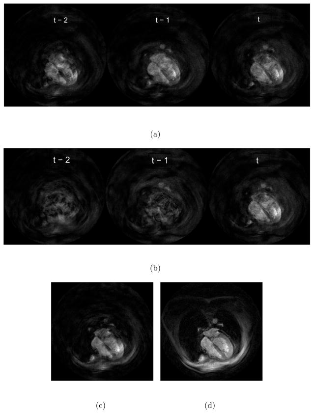
with Γ_t,t = I. While this equation is not computationally useful, it demonstrates the auto-regressive nature of the filter and the fact that aliased images are weighted within an exponential decay envelope. Indeed, this exponential behavior is more obvious when the matrices lose their time dependence under strict steady state. In this case, H_t = H so that each interleaf fully samples k-space and there is no acceleration in the reconstruction. Then, Γ_t,t′ = (I − PH^HR⁻¹H)^t−t′ and Eq. 4 becomes a matrix convolution. Figure 1 shows three most recent masked aliased images (s̃), their weighted contributions and the resulting reconstruction in an 8× experiment. The development in this subsection helps explain how the algorithm unaliases and how it can effectively handle perturbations.

Figure 1.

(a) Masked aliased images (s̃) – Notice that masking suppresses much of the aliasing artifacts by itself. (b) The respective contributions of the masked aliased images in the final reconstruction (Γ_t,t′ s̃_t′) (c) The reconstruction due only to these most recent three images ( ${\sum }_{t^{\prime }=t-2}^t{\mathrm{\Gamma }}_{t,t^{\prime }}{\stackrel{\sim }{s}}_{t^{\prime }}$) (d) The final Kalman reconstruction

2.3 Dynamic update of statistics

The previous two subsections assumed that an accurate estimate of motion statistics is available at all times. In practice, obtaining such information is a challenge even in a steady state. Performing a separate training scan corresponds to assuming wide-sense stationarity and is commonly used in dynamic imaging [5, 7, 11]. Nevertheless, this approach nullifies the flexibility expected from real-time imaging. One solution would be to embed the calibration points into the actual scan. However, care must be taken to keep the calibration points the same in all interleaves, and the resulting overhead may not be acceptable.

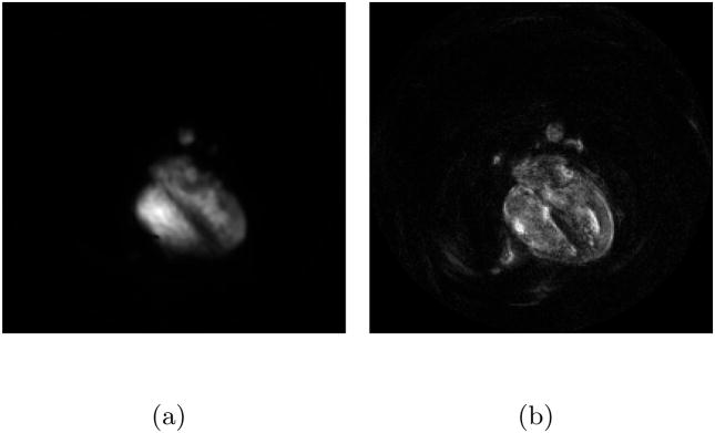
In this paper, we propose to obtain the motion map dynamically from a causal buffer of conventional images. These images are reconstructed by the regular gridding algorithm using a density compensation function. They merely support a low frame rate and therefore suffer from temporal blurring. On the other hand, asynchronous acquisition facilitates the use of these images in calibration because active pixels will still display significant variation. Of course, the resulting motion map will not be very accurate, but a rough estimate is enough for reasonable unaliasing. Eventually, the algorithm works by suppressing the changes in some pixels while accentuating others. Mild imperfections in the motion map will appear as local SNR degradations in the reconstruction.

The proposed method does not require extra scans or extra samples. Another advantage is that a high spatial resolution motion map is obtained. Therefore, in comparison to self calibration via additional low frequency samples, the method uses more accurate spatial information, but less accurate temporal information (Fig. 2).

Figure 2.

It is impossible to obtain a motion map of both high spatial resolution and high temporal resolution from a single scan, since the acceleration factor is bigger than 1. (a) A high temporal resolution, low spatial resolution map obtained by a separate training scan (b) A low temporal resolution, high spatial resolution map obtained from within the data. – Notice that the static tissues around the heart do not appear in the motion maps.

Maintaining a causal buffer of conventional images allows for incrementally updating the motion map rather than recalculating at each time point. Let the buffer hold N conventional images. If I₁, …, I_N are used to find Q̂_t′ and I₂, …, I_N+1 are used to find Q̂_t, then

$${\widehat{Q}}_t={\widehat{Q}}_{t^{\prime }}-\mid I_1\mid \times \mid I_1\mid +\mid I_{N+1}\mid \times \mid I_{N+1}\mid ,$$ (5)

since {u_t} is a zero-mean process. Subtraction of the acquisition noise variance can be optionally performed to suppress artifacts such as the spiral swirls [11].

The second parameter that needs to be dynamically updated is the acquisition noise variance, $\widehat{{{\sigma }_t}^2}$, which can be used to trade-off between SNR and temporal responsiveness. Moreover, individual coil SNRs can be utilized to dynamically manage the active coils by comparing them against a threshold value. The acquisition noise is thermal in nature and therefore white and Gaussian. Its variance can be dynamically updated by maintaining a causal buffer of outermost k-space samples. Let the buffer hold M k-space samples. If d_t−1, …, d_t−M are used to find $\widehat{{{\sigma }_{t-1}}^2}$ and d_t, …, d_t−M+1 are used to find $\widehat{{{\sigma }_t}^2}$, then

$$\widehat{{{\sigma }_t}^2}=\widehat{{{\sigma }_{t-1}}^2}-f({\mid d_{t-M}\mid }^2+{\mid d_t\mid }^2),$$ (6)

since {w_t} is a zero-mean process. Here, f is a multiplication factor motivated by the fact that it stabilizes the filter against the imperfections due to various approximations and that the acquisition noise estimate is treated as a trade-off parameter. Loosely put, f serves as a ‘knob’ adjusting the acceptable noise level during the experiment since the viewing experience is ultimately subjective. It reflects the relative trust in the data in comparison to the previous estimate. Finally, Q̂_t calculation must be overestimating because the time between conventional frames is (speed-up factor) times that of the desired frames. A simple first-order solution is to divide Q̂_t by a constant. However, rather than introducing another constant, we embed this adjustment into f as suggested in [11]. Thus, f serves as an umbrella parameter performing all the stabilization and subjective adjustment tasks. Although it is hard to choose an optimal value beforehand, the value of f can be adjusted during the experiment as mentioned above. The numerical value of f is meaningful only when the scalings for all the operators are known. In the Appendix, we suggest a natural scaling convention.

When the combine-then-reconstruct approach is taken, the sensitivity maps also need to be dynamically updated. This can be done using the conventional images already computed for the motion map update. As mentioned before, the reconstruct-then-combine approach can employ a sum-of-squares combination and does not need sensitivity maps.

Dynamic update is achieved by maintaining a first in-first out buffer. The size of the buffer is another design choice. While large buffers can provide better estimates and more immunity to noise, they also result in more sluggish responses to perturbations. Our experience suggests that a buffer of 20 conventional images provides good results although moderately acceptable reconstructions can be obtained by maintaining as low as 5 conventional images. Even with large buffers, initiation is not a problem because the Kalman reconstruction can start immediately, filling up the buffer very quickly on-the-go.

2.4 Choosing the Readout Trajectory

As mentioned before, the algorithm handles arbitrary readout trajectories naturally, using exactly the same computational steps. On the other hand, it is expected that certain readouts provide better results due to the approximations we introduced.

Let us analyze the problem from a mutual incoherence [19] persepective. When the sampling points are approximately equally important (incoherently distributed), the aliasing side lobes of the point spread function will not have prominent peaks (incoherence). Statistically, aliasing will appear as another source of noise. Therefore, the algorithm can assume that there is no aliasing involved in the sampling (diagonality assumption), and the apparent noise level is higher instead. This is another explanation of the multiplicative factor f. Thus, ignoring the burden in acquisition, a randomized sampling pattern should work better. This also explains discarding some of the samples in the already oversampled central part of k-space. Essentially, we are trying to prevent preferential treatment of k-space regions. For instance, a uniformly random sampling pattern will result in k-space regions that remain undersampled for a long time, with high probability. Consequently, the system will need more time points to become observable and the window interpretation suggests that a larger error will be incurred. The ideal readout sequence for our linear statistical algorithm seems to be an incoherent scheme that minimally disturbs observability. Poisson disk sampling is an excellent example, as used in [20]. Designing such randomized 2-D readout trajectories is considerably harder in MRI although randomizing the positions in the phase encode direction in echo-planar imaging (EPI) is convenient. This would provide a 1-D version of the algorithm. In this paper, we chose spiral readout trajectories as convenient and conventional waveforms that are also relatively incoherent in both Cartesian dimensions.

It is interesting to note that ideas from the nonlinear, ℓ₁-based compressive sensing paradigm [21] are used in a linear ℓ₂-based Kalman filtering problem. In the Appendix, we provide two basic readout trajectory/point spread function examples.

2.5 Reconstruction Complexity

The computations performed in the algorithms mentioned in this paper are dominated by grid-ding and 2-D Fourier operations. All the other computational steps require negligible resources. Therefore, they are ignored in complexity calculations.

The sliding window reconstruction uses one undersampled gridding and one 2-D Fourier operations per image. The Kalman algorithm performs two undersampled gridding and two 2-D Fourier operations per image, when the statistics are precalculated. The auto-calibrating Kalman algorithm obtains and maintains the statistics during the experiment. For an acceleration factor of a, this dynamic update requires one full gridding and one 2-D Fourier operations every a images. That is, the auto-calibrating Kalman algorithm performs 2 + 1 = 3 undersampled gridding and (2 + 1/a) 2-D Fourier operations per image. Thus, the proposed method is less than three times computationally demanding than the sliding window algorithm. The latency of the proposed algorithm is equal to the reconstruction time, unlike the sliding window algorithm which also waits for neighboring future data.

We note that the resources required for gridding depend critically on the width of the gridding kernel and the grid oversampling ratio. Beatty et al. [14] showed that desired gridding performances can be achieved by different kernel widths and fractional oversampling ratios, resulting in significant computational savings.

3 Experiments

Free-breathing, untriggered dynamic cardiac imaging experiments were performed on a 1.5T GE Signa system, using the GE 8-element cardiac array that wraps around the torso. Informed consent was obtained from the healthy volunteers before in-vivo experiments. A fat-suppressed 30° flip angle GRE excitation was used. Slice thickness was 4.7 mm. Data was acquired using the RTHawk real-time system [22]. Offline reconstructions were performed both with the proposed algorithm and the sliding window algorithm for comparison. The sliding window reconstructions accessed the available sensitivity and coil noise estimates to achieve SNR optimality. These two algorithms are both real-time capable, and have similar reconstruction complexity and latency. The first experiment was also reconstructed with the original Kalman algorithm by acquiring a separate training scan.

For the first experiment, an oblique slice of the upper torso, going through the four-chamber view of the heart is selected to visualize the rapid valvular motion. The FOV is thus set as 42 cm. The in-plane resolution is 2 mm and TE/TR = 3.8 ms/23.9 ms. Two channels of the 8-element array (lower-back side) were turned off due to insufficient sensitivity. Oversampled low frequency k-space data is discarded in the Kalman filter based reconstruction to maintain an approximately uniform sampling, as discussed in Section 2. In total, 3.3% of the acquired data was discarded. The sliding window reconstruction used all of the acquired data. An 8-interleaf spiral trajectory was used, where each interleaf corresponds to a different time point, resulting in 8× accelerated reconstructions. The buffer size was 15 conventional images (less than 3 seconds). For this experiment, we also acquired single-shot, low-resolution (6.6 mm in-plane) initialization data with the same scanner configuration. Scan durations were chosen as approximately 10 seconds to include common bulk motions such as breathing. A conventional (no acceleration) reconstruction runs at approximately 5.2 frames per second (fps) so that 8× accelerated reconstructions run at 41.8 fps. The trade-off parameter f was set as 8 for the reconstruction using separate training data, and it was set as 20 for the auto-calibrating reconstruction, as discussed in Section 2.3. We emphasize that the numerical values are meaningful only when the operator scalings are known (See the Appendix.).

We performed another experiment to test the adaptiveness of the proposed algorithm. This time, only four channels of the 8-element array were active and the imaging FOV is thus reduced to 34 cm. The in-plane resolution is 2 mm and TE/TR = 3.8 ms/22.5 ms. The Kalman filter based reconstruction discarded 3.8% of the acquired data (from the oversampled center) to achieve an approximately uniform sampling. The sliding window reconstruction used all of the acquired data. A 7-interleaf spiral trajectory was used, corresponding to 7× accelerated reconstructions. The experiment started with a four-chamber view. During the experiment, the imaging slice is altered twice. First, a 90° rotation is applied. Then, the slice is shifted to center the heart within the FOV. Thus, it was possible to assess the adaptiveness by observing the reconstructions around these big perturbations. The 7× accelerated reconstructions run at 44.5 fps. The effective undersampling is more severe in this second experiment. Although 1/7 (instead of 1/8) of k-space samples are acquired at each point, only four channels are used. Moreover, the reconstruction FOV was set as 36 cm instead of the acquisition FOV of 34 cm. This is due to significant contributions from outside the prescribed FOV. The trade-off parameter f was thus set as 30. The buffer size was 30 conventional images (less than 5 seconds).

4 Results

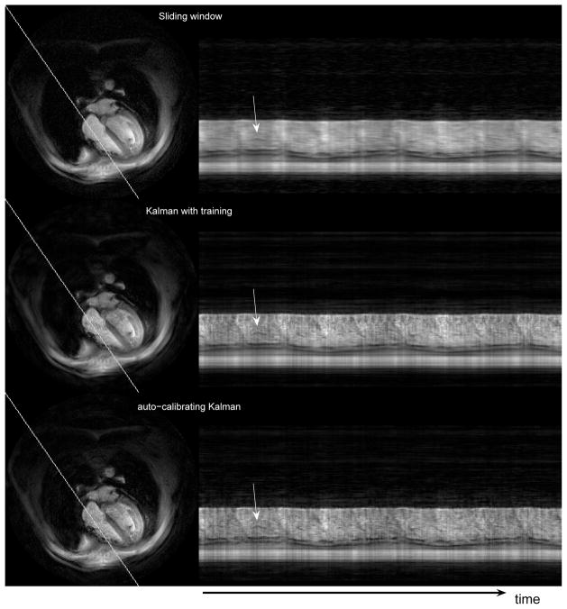
Figure 3 shows the temporal variation of an oblique line passing through the right half of the heart, from the first experiment. The representative cardiac images on the left show the position of the oblique line in the reconstructions. We compare the results obtained by the sliding window algorithm (top), the Kalman algorithm with a training scan (middle), and the auto-calibrating Kalman algorithm (bottom). The vertical position-time images on the right demonstrate two basic results: Much of the temporal blurring due to the sliding window reconstruction is resolved in both of the Kalman reconstructions and while the Kalman reconstructions do not provide identical results (due to different motion maps), there are not outstanding differences in the overall reconstruction quality. The blood pool is somewhat brighter in the middle (Kalman with training) reconstruction when compared to the bottom one (auto-calibrating Kalman), but the detail levels of the anatomical structures are about the same. The difference in the blood pool depiction can be understood by inspecting Fig 2. In GRE imaging, a proton density contrast is obtained and the blood pool appears very active due to the mixing of excited, spoiled and unexcited spins. When extra training data is used, the temporal resolution is high and the blood pool appears bright in the motion map. When a low temporal resolution map is obtained from within the actual scan, very rapid changes experience temporal aliasing and the blood pool does not appear as bright in the motion map (Fig. 2). Therefore, individual pixels around the cardiac valve may have lower crests and troughs in auto-calibrating reconstructions although the peak-to-peak variation should be higher than that of the sliding window algorithm. Low temporal resolution motion maps will result in more discrepancies at even higher acceleration factors, which is a limitation on the achievable acceleration with the proposed auto-calibration method. Naturally, different excitation sequences such as steady state free precession will have different characteristics.

Figure 3.

Temporal variation of the oblique line shown on the left side for the three reconstructions. The pixels on the oblique line are arranged vertically in the profile images. The arrows point to a certain flap of the cardiac valve. Note that the profiles are not periodic due to breathing and ungated acquisitions.

Of particular interest is the depiction of the cardiac valve. While the horizontal lines corresponding to the valve are smeared out in the sliding window reconstruction, discrete shades are visible in almost every heart beat in both of the Kalman reconstructions (arrows). Note that the dynamic imaging experiment allows the subject to breath normally and does not use gating.

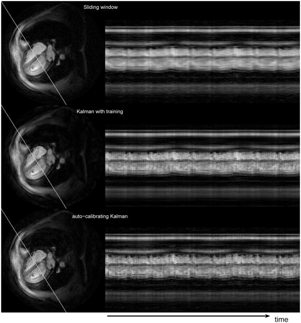
Figure 4 shows the temporal variation of another oblique line that is approximately perpendicular to the first line, again from the first experiment. The representative images on the left are rotated by 90° counter-clockwise for better visualization. The basic results mentioned in the previous paragraphs are demonstrated again. The Kalman reconstructions improve over the sliding window reconstruction in terms of the detail level in the profiles. The depiction of the rapid motion is similar in the Kalman reconstructions, the Kalman algorithm with a training scan providing a slightly brighter blood pool. We could not spot other significant differences in the pertaining videos of the Kalman algorithms.

Figure 4.

Temporal variation of the oblique line shown on the left side for the three reconstructions. The pixels on the oblique line are arranged vertically in the profile images.

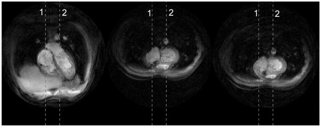
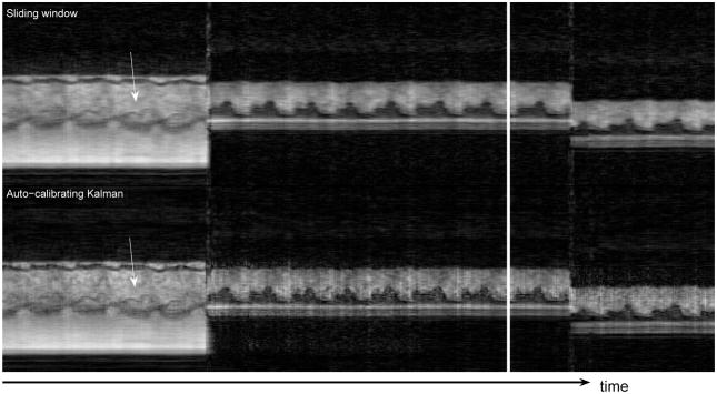
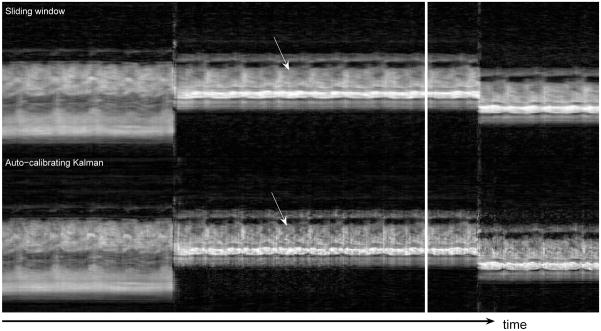
Figure 5 shows the three different views acquired during the second experiment. The temporal profiles of the vertical dashed lines are shown in Fig. 6 and Fig. 7. The top parts display the sliding window reconstruction and the bottom parts display the corresponding auto-calibrating Kalman reconstruction. Again, the depiction of the details are better in the Kalman reconstruction. Moreover, the responses of the two reconstructions to perturbations are similar. Essentially, the Kalman reconstruction gives intelligible reconstructions as soon as all of the interleaves are reacquired with the new configuration (< 160ms), which is equal to that of the sliding window reconstruction. To achieve its best, however, the Kalman reconstruction needs the buffer of conventional images to flush out all the images from the previous scenario. Figure 8 demonstrates these by concentrating on the regions of Figs. 6 and 7 where transitions happen. Although we did not implement it, one can dynamically manage the size of the buffer as well by monitoring the change between consecutive images. This should further improve the responsiveness of the Kalman reconstruction.

Figure 5.

Three different views were acquired during the dynamic imaging experiments. The first vertical dashed line goes through the valve in the first view. The second vertical dashed line goes through the valve in the second and third views. (See Fig. 6 and Fig. 7.)

Figure 6.

The temporal profiles of the first vertical dashed line in Fig 5 – Only parts of the experiments are shown for a better visualization. The Kalman reconstruction provides more detail. The arrows point to the depiction of the cardiac valve. The view change takes effect almost instantaneously in the Kalman reconstruction, essentially as fast as that of the sliding window reconstruction. The Kalman reconstruction needs a few more seconds to flush out the conventional images from the previous view.

Figure 7.

The temporal profiles of the second vertical dashed line in Fig 5 – Only parts of the experiments are shown for a better visualization. The Kalman reconstruction provides more detail. The arrows point to the depiction of the cardiac valve. The view change takes effect almost instantaneously in the Kalman reconstruction, essentially as fast as that of the sliding window reconstruction. The Kalman reconstruction needs a few more seconds to flush out the conventional images from the previous view.

Figure 8.

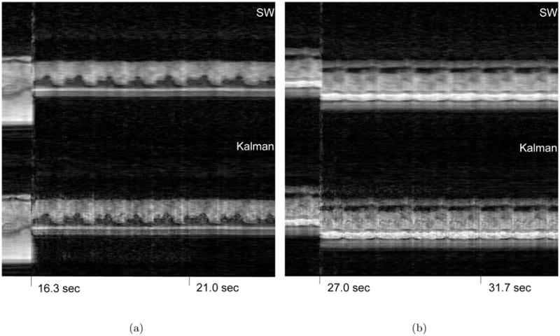
The proposed method adapts very quickly to changing conditions. However, the buffer needs to be replenished for the method to achieve its best. The effect of the previous motion maps cause artifacts until the corresponding conventional images are flushed out of the buffer. (a) The transition due to the 90° rotation (b) The transition due to the FOV shifting

It is interesting to note the manifestation of the valvular motion. In Figs. 6 and 7, the arrows point out the position of the valve in the profile. Such rapidly moving parts carry great importance in cardiac function assessment. Yet, it is exactly those parts that are smeared out by the sliding window algorithm. The improvements afforded by the auto-calibrating Kalman algorithm are readily appreciable both in these temporal profiles and in the video reconstructions.

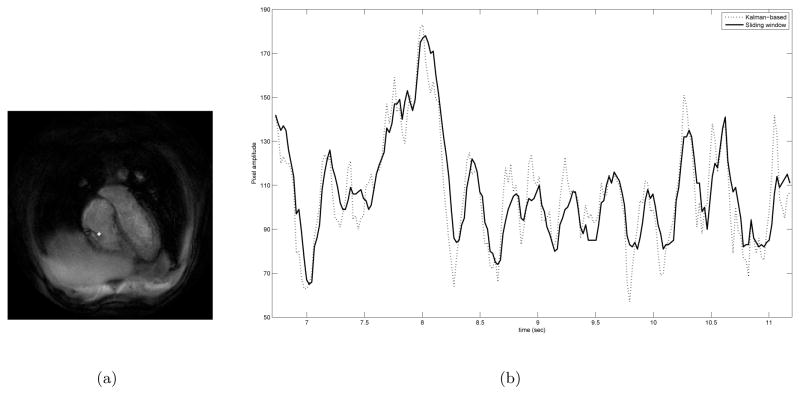
Figure 9 shows part of the time course of a single pixel that the valve leaflet sweeps through during the second experiment. The blood pool being somewhat darker in the Kalman-based reconstruction means that the corresponding plot will be shifted down a little bit. Yet, the Kalman-based reconstruction still has higher crests. More interestingly, it has quite sharper troughs when compared to the sliding window reconstruction. These troughs are the results of the dark valve leaflet sweeping through that particular pixel every once in a while. This demonstrates the improvement in quality afforded by the Kalman-based reconstruction.

Figure 9.

Comparison of the time courses of a particular pixel obtained by the sliding window and the Kalman-based algorithms (a) The position of the pixel within the FOV is highlighted. (b) Pixel intensity-time plot comparing the two reconstructions. The slight phase shift between the reconstructions is due to the noncausal window of the sliding window algorithm.

There is mild flickering in the reported reconstructions, both with the sliding window algorithm and the Kalman-based algorithm. Also, the amount of flickering is comparable between the two algorithms. Background suppression in the motion map plays a role in the amount of flickering due to the proposed algorithm. Flickering is a result of unresolved spatial aliasing caused by motion. Since our algorithm essentially provides a trade-off between rapid tracking and SNR, it is possible to get rid of such artifacts at the expense of a smoother reconstruction by increasing the noise covariance estimate. Naturally, improvements such as more involved readout trajectories should further improve the reconstruction fidelity.¹

5 Conclusions

We presented an algorithm for the real-time reconstruction of dynamic MRI acquisitions. The algorithm decreases the blur associated with the sliding window reconstruction, which is a standard method of accelerated reconstruction for real-time MRI. The algorithm builds on the original Kalman reconstruction [11] and carefully preserves causality. It is auto-calibrating so that the necessary estimates used in this statistical algorithm are obtained from within the data and in a causal manner. In addition, the algorithm provides a fast reconstruction, thereby allowing a real-time implementation.

Many real-time MRI applications involve experiments where individual images can change drastically over time. Therefore, we tested the proposed algorithm under small perturbations (breathing, patient motion, changes in coil sensitivities) and big perturbations (sudden changes in the imaging area of interest). We observed that the algorithm adapted to the new conditions very rapidly.

The algorithm merely provides a method of reconstruction and does not involve anatomical modeling. Therefore, it can be combined with other excitation pulse sequences and/or applied to other in-vivo regions of interest.

Appendix

A Scaling Convention

We now briefly describe a scaling convention. The Kalman filter does not use a density compensation function, but the calibration stage needs density compensation to reconstruct the conventional images. Let d_i denote the entries of the density compensation function, where i runs over all k-space samples. For a circular k-space coverage and an image size of n × n, one must have Σ_i d_i = π(n/2)² to preserve the amplitude of the underlying k-space function. This specification is independent of the grid oversampling ratio. Moreover, the deapodized inverse gridding reconstruction routine(H) and the deapodized gridding reconstruction routine(H^H) should be Hermitian conjugates. The same deapodization and gridding routines should be used in calibration and Kalman filtering. Note that our simplified Kalman filter requires the input samples(x_t) to be approximately uniformly distributed over k-space.

Readout Trajectory Examples

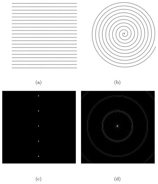
Figure 10 shows two 5× undersampled k-space readout trajectories, together with their point spread functions. The spiral trajectory (right) has an additional undersampling factor of π/4 due to its circular coverage. Slew rate limitation is disabled to discard the extra low frequency k-space samples in the spiral trajectory. Therefore, the number of samples of the spiral trajectory is indeed π/4 times that of the Cartesian trajectory (left). The point spread functions reveal that the Cartesian trajectory yields fewer but very coherent and large side lobes, whereas the spiral trajectory distributes the aliasing energy. Moreover, the changes in the phase of the point spread function also reveal the incoherency of the spiral trajectory (Fig. 11). The order in the radial direction in the spiral trajectory is also apparent in the point spread function. It is certainly possible to create more incoherent sampling patterns, but they will also be more demanding on the gradient amplifiers.

Figure 10.

5× undersampling: (a) Cartesian trajectory with 2000 samples (b) Spiral trajectory with 1574 samples (c) The absolute value of the point spread function of the Cartesian trajectory (d) The absolute value of the point spread function of the spiral trajectory

Figure 11.

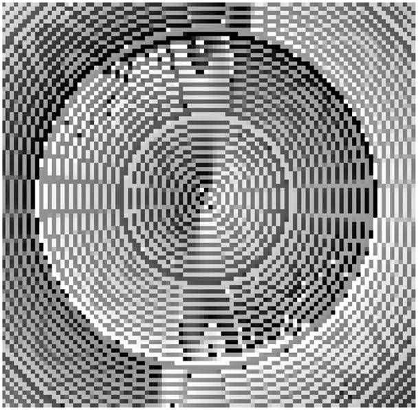
The phase of the point spread function of the spiral trajectory

References

- 1.Liang ZP, Jiang H, Hess CP, Lauterbur PC. Dynamic imaging by model estimation. Int J Imag Syst Technol. 1997;8(6):551–557. [Google Scholar]
- 2.Willis NP, Bresler Y. Lattice-theoretic analysis of time-sequential sampling of spa-tiotemporal signals .1. IEEE Trans Info Theory. 1997;43(1):190–207. [Google Scholar]
- 3.Madore B, Glover GH, Pelc NJ. Unaliasing by Fourier-encoding the overlaps using the temporal dimension(UNFOLD), applied to cardiac imaging and fMRI. Magn Res Med. 1999;42(5):813–828. doi: 10.1002/(sici)1522-2594(199911)42:5<813::aid-mrm1>3.0.co;2-s. [DOI] [PubMed] [Google Scholar]
- 4.Zhao Q, Aggarwal N, Bresler Y. Dynamic imaging of time-varying objects. Proc. ISMRM & ESMRMB Joint Annual Meeting; Glasgow: International Society for Magnetic Resonance in Medicine; 2001. p. 1776. [Google Scholar]
- 5.Tsao J, Boesiger P, Pruessmann KP. k-t BLAST and k-t SENSE: Dynamic MRI with high frame rate exploiting spatiotemporal correlations. Magn Res Med. 2003;50(5):1031–1042. doi: 10.1002/mrm.10611. [DOI] [PubMed] [Google Scholar]
- 6.Mistretta CA, Wieben O, Velikina J, Block W, Perry J, Wu Y, Johnson K, Wu Y. Highly constrained backprojection for time-resolved MRI. Magn Res Med. 2006;55(1):30–40. doi: 10.1002/mrm.20772. [DOI] [PMC free article] [PubMed] [Google Scholar]
- 7.Hansen MS, Baltes C, Tsao J, Kozerke S, Pruessmann KP, Eggers H. k-t BLAST reconstruction from non-Cartesian k-t space sampling. Magn Res Med. 2006;55(1):85–91. doi: 10.1002/mrm.20734. [DOI] [PubMed] [Google Scholar]
- 8.Lustig M, Donoho D, Pauly JM. Sparse MRI: The application of compressed sensing for rapid MR imaging. Magn Res Med. 2007;58(6):1182–1195. doi: 10.1002/mrm.21391. [DOI] [PubMed] [Google Scholar]
- 9.Jung H, Ye JC, Kim EY. Improved k-t BLAST and k-t SENSE using FOCUSS. Phys Med Biol. 2007;52(11):3201–3226. doi: 10.1088/0031-9155/52/11/018. [DOI] [PubMed] [Google Scholar]
- 10.Khalsa KA, Fessler JA. Resolution properties in regularized dynamic MRI reconstruction. 4th IEEE International Symposium on Biomedical Imaging: From Nano to Macro; Metro Washington: Institute of Electrical and Electronics Engineers; 2007. pp. 456–459. [Google Scholar]
- 11.Sümbül U, Santos JM, Pauly JM. Improved time series reconstruction for dynamic MRI. IEEE Trans Med Imag. 2009;28(7):1093–1104. doi: 10.1109/TMI.2008.2012030. [DOI] [PMC free article] [PubMed] [Google Scholar]
- 12.Bernstein MA, King KF, Zhou XJ. Handbook of MRI Pulse Sequences. San Diego: Elsevier; 2004. [Google Scholar]
- 13.Tsao J, Kozerke S, Hansen MS, Eggers H, Boesiger P, Pruessmann KP. Moving buffer k-t BLAST for real-time reconstruction: Cartesian & simplified radial cases. Proc. Intl. Soc. Mag. Reson. Med; Toronto, Canada. 2003. p. 635. [Google Scholar]
- 14.Beatty PJ, Nishimura DG, Pauly JM. Rapid gridding reconstruction with a minimal oversampling ratio. IEEE Trans Med Imag. 2005;24(6):799–808. doi: 10.1109/TMI.2005.848376. [DOI] [PubMed] [Google Scholar]
- 15.Chui CK, Chen G. Kalman Filtering with Real-Time Applications. Berlin: Springer-Verlag; 1987. [Google Scholar]
- 16.Qiu C, Lu W, Vaswani N. Real-time dynamic MR image reconstruction using Kalman filtered compressed sensing. IEEE International Conference on Acoustics, Speech, and Signal Processing; Taipei, Taiwan: Institute of Electrical and Electronics Engineers; 2009. [Google Scholar]
- 17.Pruessmann KP, Weiger M, Scheidegger MB, Boesiger P. SENSE: Sensitivity encoding for fast MRI. Magn Res Med. 1999;42(5):952–962. [PubMed] [Google Scholar]
- 18.Griswold MA, Jakob PM, Heidemann RM, Nittka M, Jellus V, Wang J, Kiefer B, Haase A. Generalized autocalibrating partially parallel acquisitions (GRAPPA) Magn Res Med. 2002;47(6):1202–1210. doi: 10.1002/mrm.10171. [DOI] [PubMed] [Google Scholar]
- 19.Donoho DL, Elad M, Temlyakov VN. Stable recovery of sparse overcomplete representations in the presence of noise. IEEE Trans Info Theory. 2006;52(1):6–18. [Google Scholar]
- 20.Lustig M, Alley M, Vasanawala S, Donoho DL, Pauly JM. L1 SPIR-iT: Autocal-ibrating Parallel Imaging Compressed Sensing. Proc. Intl. Soc. Mag. Reson. Med; Honolulu, Hawai’i. 2009. p. 379. [Google Scholar]
- 21.Candès EJ, Romberg J, Tao T. Robust uncertainty principles: Exact signal reconstruction from highly incomplete frequency information. IEEE Trans Info Theory. 2006;52(2):489–509. [Google Scholar]
- 22.Santos JM, Wright GA, Pauly JM. Flexible Real-Time Magnetic Resonance Imaging Framework. 26th Annual Int. Conference IEEE EMBS; San Francisco: Institute of Electrical and Electronics Engineers; 2004. p. 1048. [DOI] [PubMed] [Google Scholar]