Abstract
Temperature estimation in proton resonance frequency (PRF) shift MR thermometry requires a reference, or pretreatment, phase image that is subtracted from image phase during thermal treatment to yield a phase difference image proportional to temperature change. Referenceless thermometry methods derive a reference phase image from the treatment image itself by assuming that in the absence of a hot spot, the image phase can be accurately represented in a smooth (usually low order polynomial) basis. By masking the hot spot out of a least squares (ℓ2) regression, the reference phase image’s coefficients on the polynomial basis are estimated and a reference image is derived by evaluating the polynomial inside the hot spot area. Referenceless methods are therefore insensitive to motion and bulk main field shifts, however, currently these methods require user interaction or sophisticated tracking to ensure that the hot spot is masked out of the polynomial regression. This article introduces an approach to reference PRF shift thermometry that uses reweighted ℓ1 regression, a form of robust regression, to obtain background phase coefficients without hot spot tracking and masking. The method is compared to conventional referenceless thermometry, and demonstrated experimentally in monitoring HIFU heating in a phantom and canine prostate, as well as in a healthy human liver.
Keywords: Interventional MRI, Thermometry, Robust Regression, Thermal Therapy
Introduction
As an alternative to surgery, minimally invasive thermal therapies are currently under investigation for the treatment of tumors in organs such as the prostate and liver. However, a requirement for the use of any thermal therapy is the ability to monitor treatment in order to measure thermal dosage and avoid damage to surrounding tissue. MRI is a particularly promising candidate for monitoring thermal treatment, since it provides high resolution temperature maps of tissue in near real time. Though temperature influences several MR tissue parameters, the proton resonance frequency (PRF) shift with temperature is currently the favored contrast mechanism for MR thermometry. This is because the PRF shift is relatively linear over the temperature range of interest, with a constant of proportionality that is largely constant between tissue types (with the exception of fatty tissue), and because of the high spatial and temporal resolution with which PRF shift temperature maps can be acquired (1–3).
The most straightforward method for estimating temperature using the PRF shift is baseline subtraction. In that method, temperature is estimated using the phase difference between images during and prior to thermal treatment. However, baseline subtraction is highly sensitive to motion, which leads to spatial misregistration, and bulk main field changes, which incorrectly bias the temperature estimate up or down. As an alternative, referenceless methods (4–6) derive pretreatment phase in a heated region from the phase of tissue surrounding the region. Operating under the assumption that the image phase directly surrounding a hot spot would otherwise extend smoothly into the region occupied by the hot spot, referenceless thermometry methods use least-squares (ℓ2) regression to fit a low-order polynomial to the surrounding phase. The polynomial is then evaluated at locations within the hot spot, and the result is used as a reference for subtraction. Because referenceless thermometry derives temperature maps from a single image, they are immune to registration errors; however, practical implementations of referenceless methods are not entirely insensitive to motion. This is because in order to prevent the hot spot from biasing the background polynomial phase regression and causing temperature underestimation, conventional referenceless methods require that the hot spot be masked out of the regression. This means that the hot spot’s location must either be known a priori, or it must be tracked (7).
We introduce a new referenceless thermometry method that improves upon current reference-less thermometry methods by implementing reweighted ℓ1 polynomial regression (8), instead of masked ℓ2 regression. Compared to masked ℓ2 thermometry, the new method does not require the user to have a priori knowledge of the hot spot’s location in order to obtain an accurate temperature map, nor does it require sophisticated tracking techniques to follow the hot spot’s location during motion (7). We will demonstrate the new method in simulations and experiments, and show that it produces equivalent temperature maps as masked ℓ2 thermometry, without requiring knowledge of the hot spot’s location.
Algorithms
ℓ1 thermometry
Referenceless PRF shift thermometry typically uses Gradient Echo (GRE) images as input data. After excitation in a GRE sequence, magnetization phase evolves as the integral of frequency offset. Neglecting global offsets, the phase of the reconstructed image, φ(x; y), is equal to the magnetization phase at the echo time (TE), plus phase shifts applied by the receiver coil. In the absence of therapy-induced temperature change, one may assume that the pretreatment image phase θ(x; y) is smoothly-varying over large image regions, since sources of phase variation (main field variations, susceptibility changes due to lung filling, transmit and receive coil phase variations) are smooth functions of x and y. It can therefore be accurately represented by the superposition of low-order polynomials of the form:
| [1] |
Because thermal therapy is by nature spatially localized, and because the target region is generally much smaller than the imaging field of view (FOV), regions of temperature change will comprise a minority of image voxels, and will not be well-represented by low-order polynomials. In referenceless thermometry, estimates â of the coefficients ai, i = 0, …, Nb − 1, where Nb is the number of polynomial basis functions, are obtained via regression. In this context, the phases of spatial points within the hot spot may be regarded as outliers whose influence on the estimates âi is to be avoided.
ℓ1 regression is a technique commonly used in statistical analysis to avoid the influence of outliers in data (9, 10). Mathematically, the ℓ1 regression problem for PRF shift thermometry may be stated as:
| [2] |
where the length-Nb vector a contains the polynomial coefficients, I (x, y) is the complex-valued image, the vector contains the image phase at the Ns fitted spatial locations, and the Ns × Nb matrix X contains the polynomial basis functions of Eq. [1], evaluated at the points (xn, yn). Image magnitude weighting provides robustness to noise such as “popcorn” noise outside the object. This problem can be solved using methods such as linear programming (11) and iteratively-reweighted least-squares (12). We will use the iteratively-reweighted least-squares algorithm of Ref. (12) in our implementation.
Reweighted ℓ1 thermometry
While solving Eq. [2] will yield background phase estimates that are more robust to the presence of the hot spot than conventional (masked ℓ2) referenceless thermometry, we can further reduce the hot spot’s influence using iterative reweighted ℓ1 regression (8) to approximately solve an ℓ0 regression problem. Reweighted ℓ1 thermometry is implemented by the following algorithm:
Set l = 0 and W0 = diag (|I (xn, yn)|).
- Solve the weighted ℓ1 minimization problem
[3] - Update the weights by setting r = θ − Xâl, and set
[4] Terminate if l = lmax, the maximum number of reweights. Otherwise, go to 2.
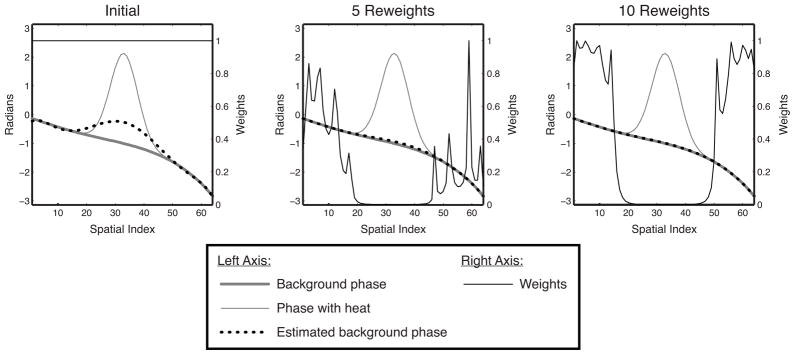
We set ε = 0.01. Figure 1 illustrates how reweighting enhances hot spot rejection by downweighting spatial locations where previous fits resulted in a large residual error.
Figure 1.
Reweighting illustration. Initially, the estimated background phase is biased significantly towards the hot spot. However, because the residual is highest in the hot spot, that area is increasingly downweighted in subsequent reweights, while the fit outside the hot spot becomes increasingly accurate. After 10 reweights, the hot spot is masked out entirely, and the background phase has been accurately estimated.
Reweighted ℓ1 thermometry without phase unwrapping
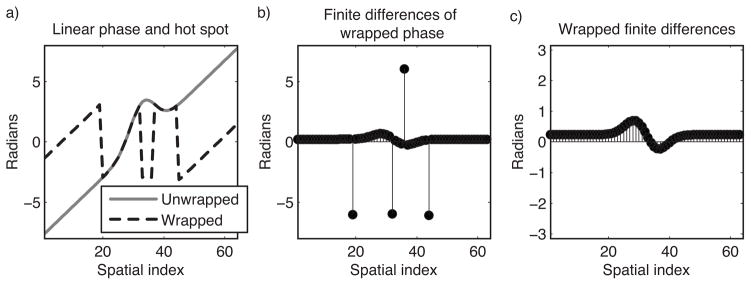
The reweighted ℓ1 thermometry method can be applied to wrapped phase images that are finite difference-filtered, to obviate phase unwrapping. Figure 2 illustrates the concept behind this extension. Figure 2a plots an unwrapped phase profile comprising a hot spot and a linear background phase, and the wrapped profile; note the four phase wraps. When first-order finite differences are calculated in each image dimension, the phase wraps become spikes, as shown in Fig. 2b. Wrapping the spikes back into the interval (−π, π) yields the wrapped finite-differenced phase shown in Fig. 2c. Reweighted ℓ1 thermometry can be performed using wrapped finite-differenced phase by solving for the coefficient vector âl that is jointly optimal in both finite-differenced image dimensions; i.e., we replace Eq. [3] with:
| [5] |
where θ̃x and θ̃y are the wrapped finite-differenced phase images, with differences taken in x and y dimensions, respectively. The diagonal weighting matrices and are calculated using the residuals rx = θ̃x − X̃xâl, and ry = θ̃y − X̃y âl respectively. Note that the zeroth-order polynomial becomes a vector of zeros after finite differencing, and is therefore excluded from the finite-differenced basis matrices X̃x and X̃y. The zeroth-order coefficient can be obtained by repeating non-finite-differenced reweighted ℓ1 thermometry with X set to a single vector of one’s, after subtracting the other estimated polynomials from the treatment image phase.
Figure 2.
Concept underlying finite difference-based reweighted ℓ1 thermometry. (a) A Gaussian hot spot superimposed on a linear background phase, unwrapped and wrapped. Conventionally, referenceless thermometry is performed after phase unwrapping. (b) In the finite differences of the wrapped phase profile, the linear ramp becomes a constant, the hot spot becomes positive and negative humps, and spikes appear at the phase wrap locations. (c) Wrapping the finite differenced phase back into the interval (−π, π) removes the spikes, and reweighted ℓ1 thermometry with finite differenced basis functions can be applied directly to this data, obviating phase unwrapping.
Finite difference-based reweighted ℓ1 thermometry is related to existing minimum norm approaches to phase unwrapping that operate in a similar manner (13, 14). We will demonstrate it in prostate thermal ablation data, where we will show that it is robust to phase spikes that arise in the finite-differenced phase between the prostate and fatty regions adjacent to it. It should be noted that in aqueous tissues, the conventional masked ℓ2 method is also compatible with finite-differenced phase.
Conversion to temperature
Upon termination of the reweighted ℓ1 thermometry algorithm, a temperature map T (xn, yn) can be obtained by subtracting the estimated background phase θ̂ (xn, yn) = { Xâ}n from the image phase, and scaling as:
| [6] |
The constant c is given by:
| [7] |
where α = −0.01 ppm/°C is the PRF change coefficient for aqueous tissue, γ is the proton gyromagnetic ratio, B0 is the main magnetic field strength, and TE is the echo time of the GRE sequence.
Numerical Simulations
We performed several simulations to investigate the influence of the number of reweights, hot spot characteristics, and background phase characteristics on reweighted ℓ1 temperature estimates. In each simulation, the new algorithm is compared with results obtained using the conventional masked ℓ2 method of Ref (4). We also investigated the potential benefit to using hot spot masking with the reweighted ℓ1 algorithm.
Simulation Setup
All simulations were performed in MATLAB (MathWorks, Inc., Natick, Massachusetts, USA) on a circular object of uniform image magnitude, defined on a 64×64 grid. The object’s background phase was synthesized from a weighted sum of polynomial basis functions with random weights. To the object’s background phase we added a Gaussian hot spot of magnitude π radians. With the exception of the hot spot location simulation, the hot spot’s size (defined as the ratio of its area above 1% of its peak value to the object’s area) was varied from 0.05 to 0.5. The masked ℓ2 method used a circular hot spot mask whose boundary was set at 2.8 standard deviations from the hot spot’s center. With the exception of the reweight number simulation, the reweighted ℓ1 method used 25 reweights and ε = 0.01. Background polynomial estimation error was quantified in terms of phase bias, which we define as the difference between the true peak hot spot magnitude (π radians) and the estimated hot spot peak magnitude. This measure reflects how much the the background polynomial fit was biased towards the hot spot, and is linearly proportional to the amount by which temperature is underestimated in the hot spot’s center. To give the reader a sense of the magnitude of these errors, at a main field strength of 1.5T and a TE of 20 ms, a 0.1 radian phase bias would correspond to a temperature underestimation of 1.24°C.
Simulation Results
Hot spot size and polynomial order
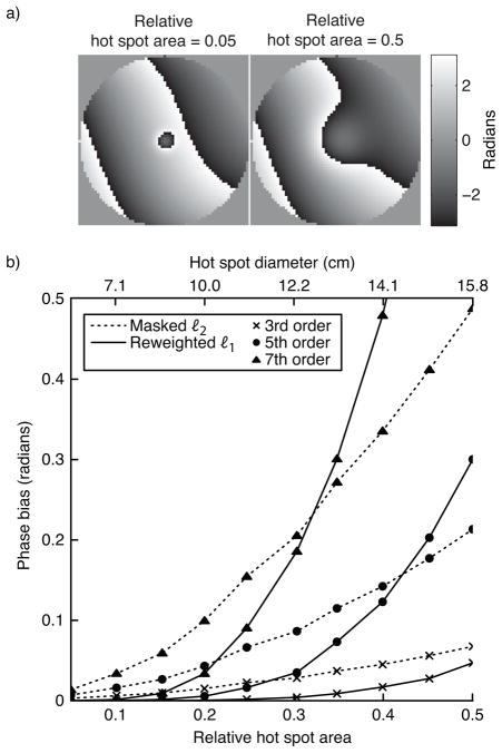
In the first simulation we tested both methods’ sensitivity to hot spot size and background phase polynomial order. The hot spot’s 1%-of-peak relative area was varied from 0.05 to 0.5, and the maximum background phase polynomial order was 3, 5, or 7. Figure 3 plots the results of this simulation. To give the reader a practical sense of the hot spots’ sizes, the plot shows the spots’ diameters (defined as the diameter of voxels above 1% of peak magnitude) if the object had a diameter of 20 cm. The figure shows that the reweighted ℓ1 method (with 25 reweights) achieves significantly smaller phase bias than the masked ℓ2 method for smaller hot spots. For both methods, error increases with background polynomial phase order. For a fixed hot spot size, error increases for large polynomial orders because the magnitude of the projection of the hot spot onto the subspace spanned by the polynomial basis increases as more high-order terms are added to the basis set. Conversely, for a fixed polynomial order, error increases with hot spot size because the hot spot becomes smoother, so its projection onto the lower-order polynomials increases in magnitude. The error of the masked ℓ2 method increases approximately linearly with hot spot area, while the reweighted ℓ1 method’s error increases exponentially. Therefore, fitting to an area much larger than the hot spot itself is crucial to the success of the reweighted ℓ1 method, when success is defined as achieving an error that is equal to or lower than that achieved by the masked ℓ2 method.
Figure 3.
Hot spot size simulation results. (a) The smallest and largest hot spot sizes, superimposed on a 5th-order polynomial background phase. (b) Error, in terms of phase bias, of the ℓ2 method and the reweighted ℓ1 method, for three polynomial orders.
Number of reweights
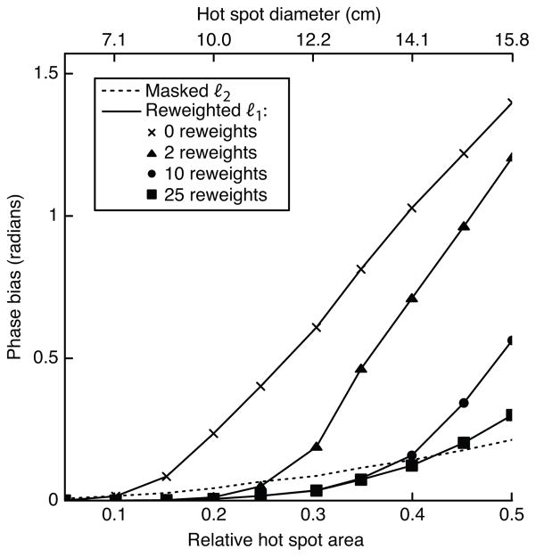
Figure 4 plots the error achieved by the masked ℓ2 method, and the reweighted ℓ1 method with 0, 2, 10, and 25 reweights, versus hot spot size for a 5th order background polynomial. The plot shows that ℓ1 referenceless thermometry benefits significantly from reweighting. Using a large number of reweights improves the reweighted ℓ1 method’s accuracy dramatically for large hot spot sizes. The number of reweights necessary to reach low bias is reasonably small across the simulated range of hot spot sizes.
Figure 4.
Error vs. number of reweights, with a 5th order polynomial background phase. For small hot spot sizes, the reweighted ℓ1 method achieves low error with a small number of reweights. As the hot spot grows larger, increasing the number of reweights results in significant improvements in accuracy.
Hot spot masking
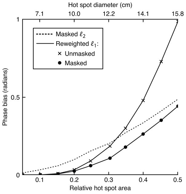
Figure 5 compares the masked ℓ2 method with the reweighted ℓ1 method without and with hot spot masking, for a 7th order background polynomial phase and 25 reweights. Hot spot masking can be used with the reweighted ℓ1 method to improve accuracy, particularly when the hot spot is very large. In this case, masked reweighted ℓ1 thermometry achieves lower phase bias than the masked ℓ2 method across the entire range of hot spot sizes.
Figure 5.
Masked reweighted ℓ1 thermometry with a 7th order background polynomial phase and 25 reweights. For each hot spot diameter, reweighted ℓ1 thermometry was applied using the same hot spot mask as in the masked ℓ2 method. Using a mask improves the accuracy of the reweighted ℓ1 method at the largest hot spot sizes, resulting in lower bias than the masked ℓ2 method across the entire range of sizes.
Hot spot shift
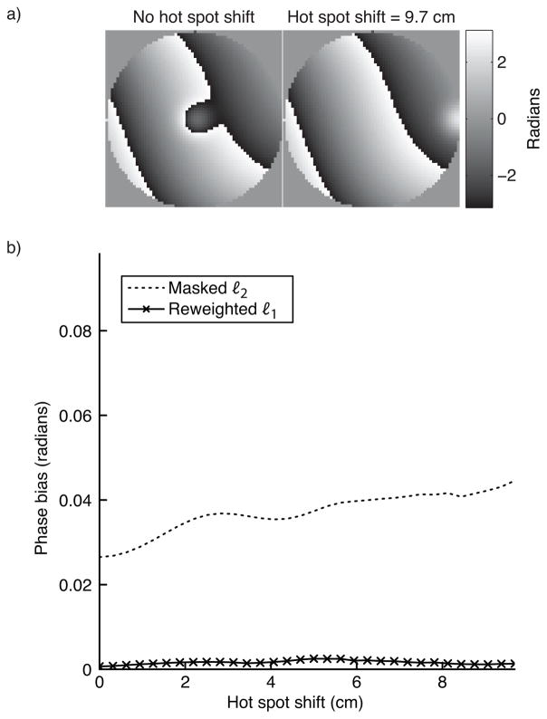
To test both methods’ sensitivity to hot spot placement within the object, we estimated the background phase for a range of hot spot displacements, up to half the simulated FOV (10 cm in a 20 cm object). The hot spot’s relative area was 0.15 (diameter 8.6 cm), and the background phase had a maximum polynomial order of 5. For the masked ℓ2 method, the mask was displaced along with the hot spot. Figure 6 shows that neither method’s accuracy is significantly impacted by the hot spot’s location within the object.
Figure 6.
Hot spot shift simulation results. Neither the ℓ2 method, or the reweighted ℓ1 method are significantly sensitive to the hot spot’s location. Both methods’ error is very low across the shift range.
Experimental Data
We applied reweighted ℓ1 thermometry to four experimental datasets, both with and without heating, in order to validate the method and demonstrate some of its advantages over the masked ℓ2 method. Prior to thermometry, in all experiments excepting the canine prostate experiment with finite-difference based reweighted ℓ1 processing, phase images were unwrapped using Goldstein, Zebker, and Werner’s algorithm (15).
HIFU heating of a gel phantom
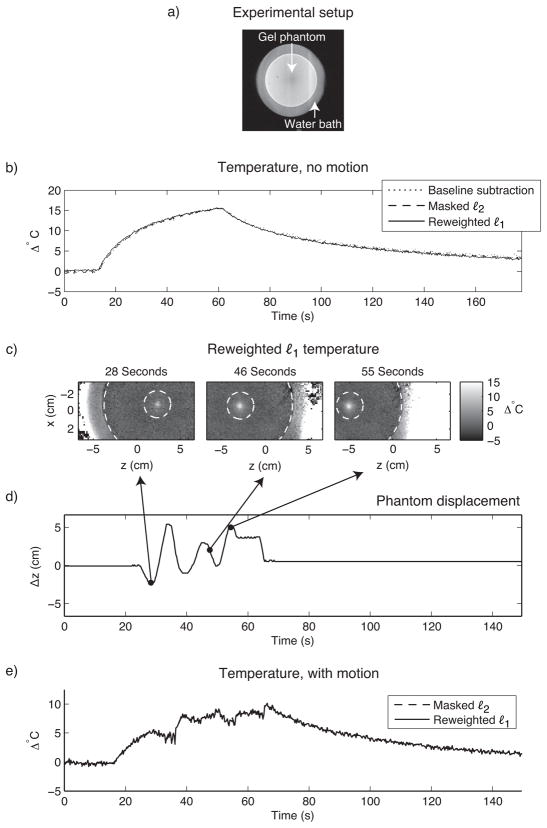
The first dataset comprised two time series of images acquired during HIFU heating of a gel QA phantom. Heating was performed using an Insightec ExAblate 2000 HIFU system (InSightec Ltd., Tirat Carmel, Israel) (50 second duration, 500kHz, 40W acoustic power). Imaging was performed on a GE 3T Signa Excite Scanner (GE Healthcare, Waukesha, WI) using a three shot readout-segmented reduced-FOV EPI sequence (TE = 16.2 ms, TR = 122 ms, 366 ms/image) (16). Both referenceless methods used a 4th order polynomial basis set, the order of which was chosen to minimize error between the temperature curves estimated by the referenceless methods and baseline subtraction in the time series with no motion. The masked ℓ2 method used an annular hot spot mask with inner diameter 3 cm and outer diameter 12 cm, whose boundaries are indicated by the dashed circles in Fig. 7c. The reweighted ℓ1 method used no masking, 25 reweights and ε = 0.01.
Figure 7.
HIFU heating of a gel phantom. (a) The experimental setup. To monitor heat, sagittal GRE images were acquired of a gel QA phantom (12 cm diameter) that was immersed in a water bath, and placed on top of a HIFU array. Heat was applied in the center of the phantom. (b) When the phantom’s position is held fixed, the referenceless methods estimate the same temperature at the hot spot center as baseline subtraction. (c) Temperature images during motion show the hot spot’s evolution and the boundaries (dashed white circles) of the hot spot mask used by the masked ℓ2 method. (d) The phantom’s displacement, obtained via manual tracking. (e) The masked ℓ2 and reweighted ℓ1 methods estimate the same temperature during motion (temperature curves coincide).
In the first time series, the phantom’s position was held fixed, and baseline subtraction was applied to the data in addition to the two referenceless methods. Figure 7b plots the temperature estimated by the three methods in the hot spot’s center. The curves are equivalent, validating the accuracy of the referenceless methods. In the second time series, the phantom and HIFU array were moved in and out of the scanner during heating, over a range of roughly 7.5 cm. For the masked ℓ2 method, the hot spot’s location was manually tracked in these images in order to center the hot spot mask. Figure 7e shows that the reweighted ℓ1 method achieves equivalent temperature estimates to the masked ℓ2 method, without hot spot tracking.
Canine prostate HIFU ablation
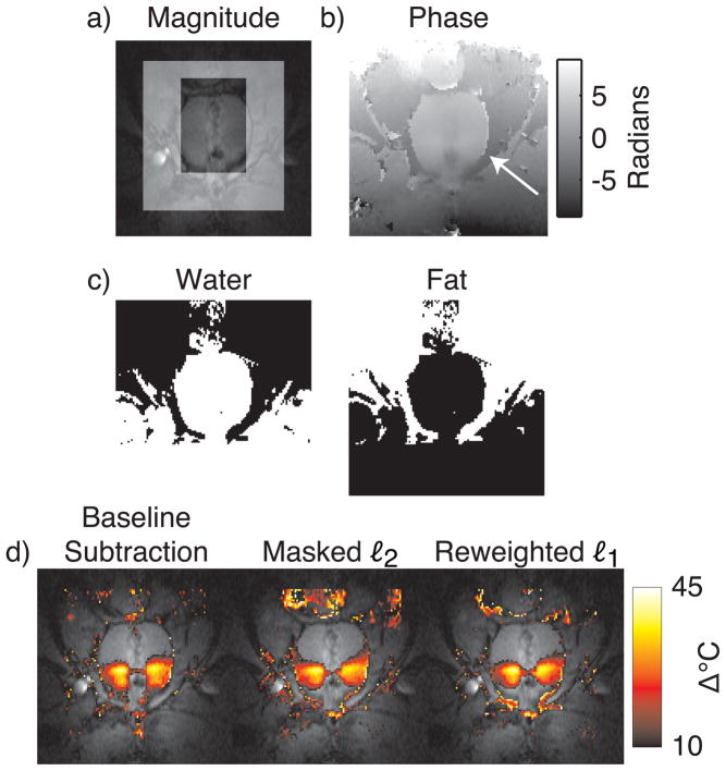
Monitoring HIFU ablation in the prostate with referenceless methods is complicated by the small size of the organ relative to typical hot spot sizes, and by the fatty tissues surrounding the organ (Fig. 8, top and middle rows). To permit polynomial fitting to a larger region around the prostate, Rieke et al proposed a modified referenceless method (6) that uses a multi-echo acquisition to derive a binary mask of the predominantly fatty tissues around the organ. Given this mask, polynomial fitting is then performed on an image from a single echo, but an additional constant phase shift is permitted within the fat mask. While the method improves upon conventional masked ℓ2 thermometry in the prostate, it requires careful frame placement to ensure that the region for fitting includes some aqueous tissue (6).
Figure 8.
Canine prostate HIFU ablation. (a) Magnitude image during heating, with the masked ℓ2 method’s mask indicated by the highlighted region. (b) The unwrapped phase image used for thermometry. As indicated by the arrow, large phase discontinuities exist at the boundary of the aqueous prostate and the fatty tissue surrounding it. (c) Water and fat masks, derived from multiecho image data. The fat mask was included as an additional basis function in the masked ℓ2 and reweighted ℓ1 method, to permit an additional global phase shift in this region, relative to the water regions. (d) Temperature estimates overlaid on the GRE image. Both referenceless methods estimate temperature maps that are similar to the baseline subtraction estimate, but the reweighted ℓ1 method does not require careful placement of a frame around the prostate.
To demonstrate that the reweighted ℓ1 method (modified to include a fat phase shift mask) produces accurate temperature estimates during prostate HIFU ablation without requiring careful frame placement, we compared the method to baseline subtraction and the modified masked ℓ2 method of Ref. (6), when applied to multi-echo images of in vivo canine prostate HIFU ablation. The dataset contained no significant motion. Images were acquired at 0.5T with an endorectal coil and a multi-echo sequence (TR = 150 – 180 ms, flip angle = 60°, TE1 = 14.3 ms, TE2 = 21.4 ms, TE3 = 28.6 ms, matrix size = 256 × 96, BW = 12.5 kHz). Ablation was performed using transurethral ultrasound applicators, as described in Ref. (6). The referenceless methods used a 4th order polynomial basis, the order of which chosen to minimize visual discrepancies between referenceless and baseline subtraction results. The reweighted ℓ1 method used 25 reweights and ε = 0.01. All methods used the image from the third echo (TE = 28.6 ms) for temperature estimation. Figure 8 shows that while the temperature estimates produced by the referenceless methods are very similar to the baseline subtraction result, the reweighted ℓ1 method achieved this result without requiring any masking.
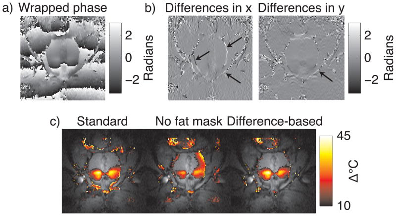
We also compared the reweighted ℓ1 method with a fat phase shift mask to the finite difference-based method. We expect that the finite difference-based method will produce accurate temperature maps in aqueous tissues adjacent to fatty tissues without knowledge of the fat/water distribution, since fatty regions experience a DC phase shift that is filtered out by finite differencing. Only phase jumps at the boundaries of fat and water regions should remain after finite differencing, which the reweighted ℓ1 method will treat as outliers and ignore. The top row of Fig. 9 shows the wrapped image phase, and the finite differences along x and y. The finite-differenced phase images contain spikes at the boundaries between fat and water, as indicated by the arrows. Reweighted ℓ1 thermometry was run on the unwrapped image phase, with and without the fat phase shift mask, using the same parameters as in the comparison above to baseline subtraction and the masked ℓ2 method. In addition, we also processed the wrapped phase using the difference-based method, using 4th order polynomials, 25 reweights, and ε = 0.01. The bottom row of Fig. 9 shows the estimated temperature maps. Without a fat phase shift mask, the reweighted ℓ1 method is biased heavily towards the phase in the fatty regions around the prostate, resulting in significant temperature underestimation (Fig. 9, bottom row, middle image). In contrast, inside the prostate the finite differencing-based method estimates nearly an identical temperature map to the reweighted ℓ1 method. It achieved this without requiring phase unwrapping or knowledge of the fat/water distribution in the image. Therefore, the method permits background polynomial fitting to a large region around the prostate, without requiring a multi-echo acquisition.
Figure 9.
Comparison of standard reweighted ℓ1 thermometry to finite difference-based reweighted ℓ1 thermometry in the same canine prostate data as in Fig. 8. The top row shows (a) the wrapped image phase, and (b) the finite differences in the x and y dimensions. The finite difference images are relatively flat, with the exception of spikes at boundaries between fat and water (arrows). The bottom row (c) compares final temperature maps between standard reweighted ℓ1 thermometry with and without a fat phase shift mask, and finite difference-based reweighted ℓ1 thermometry. The finite difference-based approach yielded nearly the same map as the standard approach, without requiring unwrapping or knowledge of the fat/water distribution.
Liver
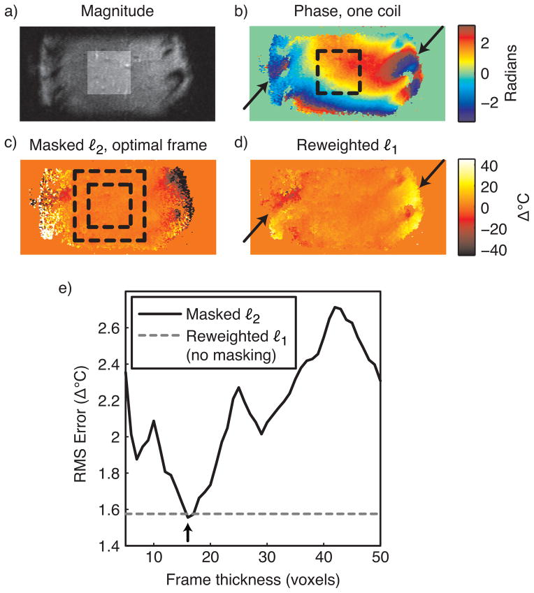
In the absence of focal heating, image phase in the liver is generally smooth, and refer-enceless thermometry is regarded as a strong candidate for monitoring thermal therapies in this organ. However, image phase in tissue surrounding the ribs adjacent to the liver contains high spatial frequencies (Fig. 10b), and care must be taken in using masked ℓ2 thermometry to avoid including these regions in the mask for polynomial fitting. To compare the performance of the masked ℓ2 and reweighted ℓ1 methods in the liver, we applied both methods to a sagittal image of a healthy volunteer’s liver, acquired using the same pulse sequence as in the gel phantom experiment. An eight channel cardiac array was used for reception. The resulting image had FOV 30 × 10 cm. A target therapy/hot spot region was selected in the center of the liver, as indicated by the highlighted region in Fig. 10a, and the inner dashed boxes of Figs. 10(b, c). We then repeatedly applied masked ℓ2 thermometry (with polynomial order 5) for frame thicknesses between 5 and 50 voxels in increments of one voxel, and measured the RMS temperature error in the target region for each thickness. Thermometry was performed separately on each coil’s image, and the resulting temperature maps were combined using an image magnitude-weighted mean. We also applied the reweighted ℓ1 method with the same polynomial order, 25 reweights and ε = 0.01, and combined the individual coil images in the same way.
Figure 10.
Liver thermometry. (a) Sum-of-squares image (sagittal view) of a healthy volunteer’s liver (no heating), with the target hot spot region highlighted. (b) The phase of one coil in the eight-channel cardiac array shows smooth phase within the liver, but rapidly-varying phase around the ribs (black arrows). (c) When the frame thickness is optimized (boundaries indicated by dashed black square), the masked ℓ2 method achieves low temperature errors in the target region (inner square), and ignores phase around the ribs. (d) The reweighted ℓ1 method also achieves low temperature errors in the target region, and ignores the phase around the ribs (black arrows). (e) The reweighted ℓ1 method achieves a temperature error that is close to that of the masked ℓ2 method with optimal frame thickness (black arrow), without requiring frame optimization.
Figure 10c shows the temperature map estimated by the masked ℓ2 method with the optimal frame thickness of 16 voxels. At this frame thickness, large temperature errors are present around the ribs, indicating that the method successfully ignored these regions in the background polynomial estimation. Figure 10d shows that the reweighted ℓ1 method also successfully ignored phase around the ribs, without masking out those regions. This behavior will extend to other scenarios in which the background phase contains features that are not well-modeled by low-order polynomials, such as regions of high local susceptibility: the reweighted ℓ1 method will ignore these features and perform an accurate phase fit in image regions that are well-modeled by the background polynomial basis. Furthermore, the plot in Fig. 10e shows that within the target region, the reweighted ℓ1 method achieved an error close to that of the masked ℓ2 method with optimal frame thickness.
Discussion and Conclusion
We have introduced a new PRF shift thermometry method based on reweighted ℓ1 regression, and demonstrated it in simulations and experimental data. The method is an iterative regression algorithm that automatically rejects the hot spot from a background polynomial phase regression by implicitly developing a spatial mask based on residual errors from previous regressions. We showed that the method estimates temperature maps of similar quality to the conventional masked ℓ2 referenceless thermometry method of Ref. (4), without requiring the hot spot to be masked and tracked. Reweighted ℓ1 thermometry therefore stands as an improvement over masked ℓ2 thermometry in terms of robustness to motion and automation.
There are extensions of the reweighted ℓ1 method that can improve its performance in different applications. First, if one has reliable hot spot tracking information, or if little motion is expected to occur during treatment, then masked reweighted ℓ1 thermometry (as demonstrated in Fig. 5) is likely to be the best approach. Compared to the masked ℓ2 thermometry, masked reweighted ℓ1 thermometry will be robust to errors in the mask placement that may result in the hot spot entering the region for polynomial fitting. Compared to the reweighted ℓ1 method without masking, masked reweighted ℓ1 thermometry will be more robust to large hot spots. We also introduced finite difference-based reweighted ℓ1 thermometry, which obviates phase unwrapping prior to referenceless thermometry. We demonstrated in a prostate heating experiment that this extension to the method also permits accurate referenceless thermometry within the organ, without knowledge of the fat and water distributions in tissues surrounding the organ. This ability will allow faster frame rates in monitoring prostate thermal therapy, since multi-echo data need not be acquired. Another approach to obviating phase unwrapping is to perform thermometry using complex images of unit magnitude but with the same phase as the original image (5). While that approach is also compatible with the reweighted ℓ1 method, the finite difference-based approach may be more attractive since working with image phase is more intuitive than separate real and imaginary parts, and since higher polynomial orders can be required to fit real and imaginary parts separately, compared to fitting the phase (5). Though their influence was not evaluated here, changes in T1 and T2 decay that result in decreased image magnitude with heat should aid the reweighted ℓ1 method in general, since this magnitude decrease further downweights phase in the hot spot during polynomial fitting.
Because it is desirable to use thermometry algorithms in real-time, a note on computation time is in order. We have found empirically that the reweighted ℓ1 algorithm requires approximately two orders of magnitude more compute time than ℓ2 thermometry, however, ℓ2 thermometry is computationally a very cheap algorithm. For example, processing a 64 × 64 image with a 7th order polynomial fit in MATLAB took 2.66 seconds with the reweighted ℓ1 method (25 reweights), and 0.023 seconds with the ℓ2 method, on a 2.6 GHz Intel Core 2 Duo laptop computer with 4 GB of random access memory. Implementation in the C programming language should reduce the compute time significantly, and it is likely that a workstation with a faster CPU and bus speed would be used in practice. Further accelerations could be made by carrying over polynomial coefficients between measurements, since the coefficients should not change significantly if no motion has occurred. In moving organs, one could build a library of initial coefficients at different phases in the motion cycle. For example, in the liver, coefficients could be stored for each phase in the respiratory cycle. These coefficients could be averaged over time using a sliding window to adapt to non-periodic phase shifts. Quadratic Tikhonov roughness penalties that penalize differences between the coefficients of adjacent time points could also be easily appended to the regression cost function to accelerate convergence. It is also possible that other algorithms exist for solving the ℓ1 regression problem that are computationally cheaper than the iteratively-reweighted least-squares algorithm used here.
The reweighted ℓ1 method requires the user to choose four parameters: the basis for back-ground phase regression, the number of reweights, ε, and the region for polynomial fitting. In referenceless thermometry, the basis for background phase regression is generally chosen to be a set of polynomials; Rieke et al (4) have described a method for choosing the polynomial order based on minimizing error within the target region for treatment, in an image acquired prior to treatment. The same approach could be used with the reweighted ℓ1 method, since the method can be thought of as an ℓ2 regression with a hot spot mask that is automatically generated. It should be noted, however, that the reweighted ℓ1 method is fully compatible with any background phase basis choice; this is also true for masked ℓ2 thermometry. In simulation we showed that the accuracy of the reweighted ℓ1 method only improves with more reweights, so this parameter could be set to the maximum number that is computationally feasible within the time constraints of real-time imaging. Alternatively, one could employ a stopping criterion to detect convergence and stop the algorithm, such as when the normalized difference between the residuals or coefficients of subsequent reweights falls below a certain percentage threshold. We have not encountered any scenarios in which too many reweights results in instability. We note however that the number of reweights required to reach a given accuracy, as well as sensitivity to variations in this parameter, will be a function of the algorithm chosen to implement the weighted ℓ1 regression. In this work, in the interest of computational speed we implemented weighted ℓ1 regression using an iteratively-reweighted least-squares algorithm that generally converges to a less optimal solution than linear programming; as a result, compared to results presented in Ref. (8) a relatively large number of reweights was required to reach an accurate result. Using linear programming to solve the weighted ℓ1 regression problem will likely require many fewer reweights (i.e., less than five), thereby reducing the burden on the user to select this parameter. We have found empirically that ε = 0.01 is a good choice in all the temperature estimation scenarios we have investigated. In general, our implementation of the method is not sensitive to variations in this parameter over about an order of magnitude (results not shown). This suggests that one could coarsely optimize ε prior to treatment by running the reweighted ℓ1 method with several values of ε (perhaps distributed logarithmically), and choosing the value that minimizes the RMS temperature error within the target treatment area. A value of ε that is much too large dampens the benefit of reweighting, and results in an estimated background phase that is biased toward the hot spot. Conversely, a ε value that is much too small could result in numerical instability. We found in simulations that fitting the background polynomial to a region much larger than the hot spot itself is crucial to the success of the reweighted ℓ1 method, when success is defined as achieving an error that is equal to or lower than that achieved by the masked ℓ2 method. In practice, the size of the region for polynomial fitting should be several times larger than the hot spot itself; as the size of the fitted region increases, the hot spot becomes less representable in the smooth background polynomial subspace, and fewer reweights are required to reach an accurate result. However, aside from this requirement our experimental results show that the fitted region can be selected less carefully for the reweighted ℓ1 method, since the hot spot and other features that may erroneously bias background phase estimation need not be interactively masked out of the region.
A topic for future investigation is joint temperature estimation when multiple receive coils are used. In the liver experiment, we performed thermometry on each coil image in isolation, and then combined the residuals in an image magnitude-weighted mean. However, it may be possible to improve hot spot rejection by averaging the residuals across coils within each reweighting step.
Acknowledgments
Support
This work was supported by NIH grants R01 CA111981, RO1 CA121163, R21 EB007715 and P41 RR009784.
References
- 1.Ishihara Y, Calderon A, Watanabe H, Okamoto K, Suzuki Y, Kuroda K, Suzuki Y. A precise and fast temperature mapping using water proton chemical shift. Magn Reson Med. 1995;34(6):814–823. doi: 10.1002/mrm.1910340606. [DOI] [PubMed] [Google Scholar]
- 2.De Poorter J, De Wagter C, De Deene Y, Thomsen C, Stahlberg F, Achten E. Noninvasive MRI thermometry with the proton resonance frequency (PRF) method: in vivo results in human muscle. Magn Reson Med. 1995;33(1):74–81. doi: 10.1002/mrm.1910330111. [DOI] [PubMed] [Google Scholar]
- 3.Peters RTD, Hinks RS, Henkelman RM. Ex vivo tissue-type independence in proton-resonance frequency shift MR thermometry. Magn Reson Med. 1998;40(3):454–459. doi: 10.1002/mrm.1910400316. [DOI] [PubMed] [Google Scholar]
- 4.Rieke V, Vigen KK, Sommer G, Daniel BL, Pauly JM, Butts K. Referenceless PRF shift thermometry. Magn Reson Med. 2004;51(6):1223–1231. doi: 10.1002/mrm.20090. [DOI] [PubMed] [Google Scholar]
- 5.Kuroda K, Kokuryo D, Kumamoto E, Suzuki K, Matsuoka Y, Keserci B. Optimization of self-reference thermometry using complex field estimation. Magn Reson Med. 2006 Oct;56(4):835–843. doi: 10.1002/mrm.21016. [DOI] [PubMed] [Google Scholar]
- 6.Rieke V, Kinsey AM, Ross AB, Nau WH, Diederich CJ, Sommer G, Butts Pauly K. Referenceless MR thermometry for monitoring thermal ablation in the prostate. IEEE Trans Med Imaging. 2007;26(6):813–821. doi: 10.1109/TMI.2007.892647. [DOI] [PMC free article] [PubMed] [Google Scholar]
- 7.Kokuryo D, Kaihara T, Kumamoto E, Fujii S, Kuroda K. Method for target tracking in focused ultrasound surgery of liver using magnetic resonance filtered venography. Conf Proc IEEE Eng Med Biol Soc. 2007;2007:2614–2617. doi: 10.1109/IEMBS.2007.4352865. [DOI] [PubMed] [Google Scholar]
- 8.Candes EJ, Wakin MB, Boyd SP. Technical report. Caltech; Pasadena, CA: 2007. Enhancing sparsity by reweighted ℓ1 minimization. [Google Scholar]
- 9.Huber PJ. Robust statistics. Wiley; New York: 1981. [Google Scholar]
- 10.Friedman J, Hastie T, Tibshirani R. Springer Series in Statistics. 2001. The elements of statistical learning. [Google Scholar]
- 11.Boyd S, Vandenberghe L. Convex Optimization. Cambridge; Cambridge, UK: 2004. [Google Scholar]
- 12.Chartrand R, Wotao T. IEEE ICASSP. Apr, 2008. Iteratively reweighted algorithms for compressive sensing; pp. 3869–3872. [Google Scholar]
- 13.Ghiglia DC, Romero LA. Minimum Lp-norm two-dimensional phase unwrapping. J Opt Soc of Am A. 1996;13(10):1999–2013. [Google Scholar]
- 14.Ghiglia DC, Pritt MD. Two dimensional phase unwrapping: theory, algorithms and software. Wiley; New York: 1998. [Google Scholar]
- 15.Goldstein R, Zebker H, Werner C. Satellite radar interferometry- Two-dimensional phase unwrapping. Radio Science. 1988;23(4):713–720. [Google Scholar]
- 16.Holbrook AB, Santos JM, Kaye E, Rieke V, Butts Pauly K. Real-time MR thermometry for monitoring HIFU ablations of the liver. Magn Reson Med. 2010;63(2):365–373. doi: 10.1002/mrm.22206. [DOI] [PMC free article] [PubMed] [Google Scholar]
- 17.Nayak KS, Cunningham CH, Santos JM, Pauly JM. Real-time cardiac MRI at 3 Tesla. Magn Reson Med. 2004;51(4):655–660. doi: 10.1002/mrm.20053. [DOI] [PubMed] [Google Scholar]


