New aspects of the elastic net algorithm for cluster analysis

Abstract

The elastic net algorithm formulated by Durbin–Willshaw as a heuristic method and initially applied to solve the traveling salesman problem can be used as a tool for data clustering in n-dimensional space. With the help of statistical mechanics, it is formulated as a deterministic annealing method, where a chain with a fixed number of nodes interacts at different temperatures with the data cloud. From a given temperature on the nodes are found to be the optimal centroids of fuzzy clusters, if the number of nodes is much smaller than the number of data points. We show in this contribution that for this temperature, the centroids of hard clusters, defined by the nearest neighbor clusters of every node, are in the same position as the optimal centroids of the fuzzy clusters. The same is true for the standard deviations. This result can be used as a stopping criterion for the annealing process. The stopping temperature and the number and sizes of the hard clusters depend on the number of nodes in the chain. Test was made with homogeneous and nonhomogeneous artificial clusters in two dimensions. A medical application is given to localize tumors and their size in images of a combined measurement of X-ray computed tomography and positron emission tomography.

Introduction

Problems of classification of groups of similar objects exist in different areas of science. Classification of patterns of genes expressions in genetics and botanic taxonomy are two out of many examples. The objects are described as data points in a multivariate space, and similar objects form clusters in this space. To find clusters without the knowledge of a prior distribution function, one uses an arbitrary partition of the data points in clusters and defines a cost functional that will then be minimized. As a result, one gets partitions of data points with optimal distribution functions of associated fuzzy clusters and their positions.

One of the most successful methods which uses this procedure is the elastic net algorithm (ENA) of Durbin–Willshaw [1] which was initially formulated as a heuristic method and applied to the traveling salesman problem. Later, it was given a mechanical statistic foundation [2, 3] and used for diverse problems in pattern research [4, 5, 6]. In this formulation, a chain of nodes interacts with given set of data points with a square distance cost or energy function. For the distribution of the data points, one uses the principle of maximum entropy that gives a probability to find the distance between data points and nodes as a function of a parameter which, in a physical analogy, is the inverse temperature. Additionally, one introduces a square distance interaction between the nodes. The total cost function is then minimized with respect to the node positions. The resulting nonlinear set of equations can be iterated with the steepest descent algorithm.

If the number of data points is much larger than the number of nodes and for a not to large node–node interaction, the interaction energy between the nodes can be treated as a perturbation. For a typical temperature, one finds than a partition of the whole cluster into several fuzzy clusters. For our calculations of cluster properties, we will use hard clusters, given by the number of nearest neighbors of every node. Fuzzy and hard clusters can then be used to define a stopping criterion for the annealing process. It gives the most optimal fuzzy and hard clusters for a given number of nodes.

We test the results by applying the annealing process and the criterion to a homogeneous and a nonhomogeneous two-dimensional cluster. An application of the algorithm to the detection of carcinoma and their size is given, analyzing medical images of positron emission tomography (PET) and computer tomography (CT) of a human lung by a combined measure PET/CT [9].

Some new aspects on the elastic net algorithm

For a given number of data points x _i in n-dimensional space, we define a chain of nodes y _j in the same space and connect the nodes with the data points by a square distance energy function.

1

Data and nodes are normalized and without dimensions. The total energy is then given by [7]

2

with the unknown probability distribution P _ij to find the distance . Putting the system in contact with a heat reservoir and using the maximum entropy principle, one finds with the constraint (2) a Gaussian probability distribution [2, 7]:

3

with the partition function for the data point i

4

Figure 1 shows for an arbitrary node j of a chain of nodes, a typical plot of P _ij versus E _ij. We have fitted a Gaussian function to the data points of P _ij, and one notes clearly that the probability distribution is of Gaussian form.

Fig. 1.

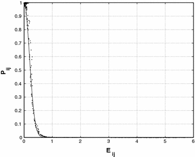
Typical form of the distribution function P _ij versus energy E _ij for an arbitrary node j. The drawn curve is a Gaussian function fitted to the data points

The parameter β is inversely proportional to the temperature and shows a probability which for high temperature associates equally with all nodes and localizes it to one node for low temperature. Using independent probabilities for every node, one finds for the total partition function:

5

and the corresponding Helmholtz free energy [7, 8],

6

where we have added an interaction energy between the nodes

7

in form of springs, with the spring constant λ. Minimization of the free energy with respect to the node positions gives for every value of β a nonlinear coupled equation for the optimal node positions:

8

We solve the equation for different β values iteratively with the steepest descent algorithm [4]:

9

with the time step ▵τ chosen adequately.

In general, we will have many data points that interact with a small number of nodes, and for a not too large spring constant, the node interaction energy will be small with respect to the interaction energy between nodes and data points and may be treated as a perturbation. To preserve the topology of the chain, we use a small node–node interaction. If we write equation (8) in the form

10

we note that for the second term in equation (10) is negligible. This is the case if around the node y _j are sufficient data points that contribute with a large probability. If there are only few data points that contribute, then some next neighbor nodes must be present in a small distance and again the second term is negligible because of the small difference of the nodes. That means that in a good approximation equation (10) reduces to

11

which represent the optimal centroids of clusters for a set of probability distributions associated with the data points. The probabilities are called “fuzzy membership in clusters” [2]. We will use the term “fuzzy clusters” for these associations. For every node, we have then the probability distribution for the associated fuzzy clusters given by

12

In the deterministic annealing method, one solves the equation (9) first for a low value of β (high temperature). Here, one should find only one cluster, the whole cluster (11) gives its centroid, and the free energy is in its global minimum. Then, one solves (9) successively for increasing β, tracing the global minimum.

Figure 2 shows schematically the annealing process for a chain of 3 nodes for 3 different values of β. For values of β < 1.4, all 3 nodes are in the same position as the centroid of the whole cluster with a constant total energy that is at a global minimum. For β between approximately 1.4 and 3.0, there is a first separation of the 3 nodes in 2 different positions describing 2 clusters. The total energy decreases abruptly to a lower constant value. From on there is a final separation of the 3 nodes in 3 different positions, giving 3 clusters. The total energy decreases sharply to a lower value.

Fig. 2.

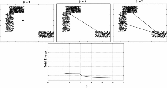
Schematic presentation of the annealing process for a cluster distribution using a chain of 3 nodes. Every node separation gives a sharp change in the total energy curve

Rose et al. [2] have shown that for the case where no node–node interaction is taken into account (), the whole clusters split into smaller clusters and one finds some of the nodes y _j as optimal centroids of the clusters. They interpret the forming of different number of clusters as phase transitions. In every phase exist a well-defined number of fuzzy clusters and one can estimate their mean size, using the Gaussian form of the probability distribution, given by (3), (4) and (1). One expects that only those data points for which on the average contribute to the clusters, with σ_c the average value of the standard deviation. This gives an average value for the mean size of the fuzzy clusters:

13

The same situation is found when the node–node interaction is taken into account as a perturbation. If there are more nodes than clusters, the rest of the nodes will be found near the nodes that correspond to the clusters. More clusters than nodes cannot be detected anymore. There exists a typical value of β, where the number of nodes is the same as the number of forming clusters. These clusters are optimal, i.e. their nodes are optimal centroids of the corresponding clusters. One would expect that these clusters are well defined in the sense that their probability distributions have large values for the data points of the clusters and go fast to zero for other data points.

To establish a criterion for finding the β value for this situation and stop the annealing process, we define a hard cluster for every node, determined by the nearest neighbor data points of the node. The centroid of the hard cluster, the hard centroid, is given by

14

where C _j forms the cluster of nearest neighbors of node y _j with n _j members. Its probability distribution H _ij is constant for its members

15

To illustrate the difference between fuzzy and hard clusters, we show in Fig. 3 for an arbitrary node a fuzzy and hard cluster (a) for a low value of β and (b) for a converged value of β. The data points of the fuzzy clusters are restricted to values of the probability distribution F _ij > 10⁻⁴.

Fig. 3.

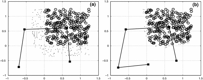
(a) A chain of 5 nodes (filled rectangles), a fuzzy cluster (dots), and a hard cluster (circles) of node 4 for a not converged annealing process (low β). (b) The same situation for the converged process. In phase (a), 2 nodes are at the same position

The hard clusters can be compared with the fuzzy clusters of the optimal situation, and one expects that fuzzy clusters and hard clusters have their best approach, i.e. their centers coincide and the range of the probability distribution of the fuzzy clusters is the same as that of the hard clusters. For this stopping criterion, we use the centroids and the standard deviation:

16

where σ_j and are the standard deviations of the fuzzy clusters and the hard clusters.

During the annealing process, one passes a series of phase transitions that are characterized by a certain number of clusters and a deformation of the chain of nodes. As the energy of the chain E _nod is generally much smaller than the interaction energy of the nodes with the data points, the change of the deformation should be of the order of the energy of the chain and E _nod shows clearly this phase changes.

In Fig. 4, we give a schematic presentation of the convergence of nodes, hard centroids, and the standard deviations of the 3 clusters during the annealing process for the same cluster distribution as in Fig. 2. For all 3 nodes are nearly at the same position (unfilled square). The 3 hard centroids have different positions because of the slightly different node positions. The standard deviations for the nodes, σ, are strongly different to the standard deviations for the hard centroids . The hard cluster with has no elements and its hard centroid coincides with one of the node positions. For we find 2 node positions and 3 hard centroids. One of the hard centroids is at the same position as one node and describes the situation that for cluster number 2 convergence has been reached. The other 2 clusters, number 1 and 3, are not separated yet, and the node describes the 2 clusters with 2 different hard centroids. The standard deviations are much closer now, and they have the same value for cluster number 2. Finally, for the 3 nodes have separated and reached the same positions as the hard centroids of the 3 clusters. The standard deviations are practically the same.

Fig. 4.

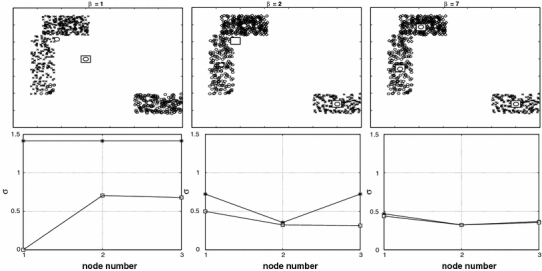
Schematic presentation of the annealing process for a cluster distribution using a chain of 3 nodes. The nodes are given by unfilled squares and the hard centroids by circles. The lower figures show the standard deviations σ of the fuzzy clusters (upper curve) and hard clusters (lower curve)

Application to artificial created two-dimensional clusters

As an illustration of the algorithm and the stopping criterion, we apply the ENA to two artificial created clusters. In the first example, cluster C1, we create a two-dimensional rectangular homogeneous cluster, and in the second example, cluster C2, we create a two-dimensional rectangular nonhomogeneous cluster with different density regions. Figure 5 shows the two clusters.

Fig. 5.

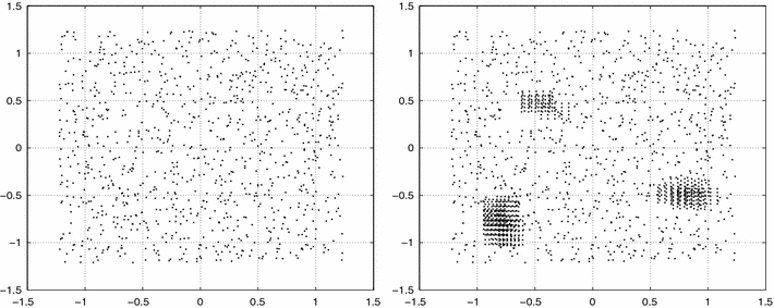
Homogeneous clusters C1 and nonhomogeneous cluster C2

We begin with a chain of 20 nodes that are localized at a small region at the center of the corresponding cluster. The β-dependent node positions and energy E _nod of the chain are then calculated with the steepest descent algorithm (9) with a time step ▵τ = 0.001. Table 1 shows the relevant data for the two clusters.

Table 1.

Number of data points and nodes, initial value β_i, final value β_f, iteration step ▵β, and spring constant λ for the cluster calculations

Cluster	Data	Nodes	βi	βf	▵β	λ
C1	1,000	20	0.001	70.0	0.001	0.1
C2	1,673	20	0.001	100.0	0.001	0.1

For the cluster C2, we needed a higher values for β to get convergence. This is a general trend, in inhomogeneous clusters the probability distributions need more iterations to get optimal because of the density changes in these regions.

Figure 6 shows the node interaction energy E _nod for the cluster C1 as a function of β. The arrows indicate the phases for which we registered the node positions, the hard centroids, the probability distributions, and the standard deviations. Figure 7 shows data points, chain of nodes, and hard centroids for the phases (a): , (b): ,(c): and (d): . Figure 8 shows the standard deviations of the fuzzy clusters, hard clusters, and the mean size σ_c of estimation (13) for the different phases of C1. To illustrate in detail the stopping criterion we show in Fig. 9 the probability distributions of node 8 for the fuzzy and hard clusters of the phases, F _i8 and H _i8. Node 8 was chosen because in its final position is in the center of the total cluster and its fuzzy cluster shows a homogeneous and isotropic data distribution

Fig. 6.

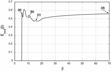
Node interaction energy E _nod as a function of β for cluster C1.The arrows indicate the phases a, b, c, d for data registrations

Fig. 7.

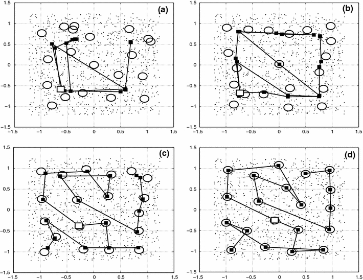
Data points (dots), nodes (filled rectangles), and hard centroids (circles) for phases a, b, c, d of cluster C1. The node 8 is marked in every phase by a square unfilled symbol

Fig. 8.

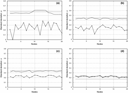
Standard deviations for fuzzy clusters, hard clusters, and the estimation σ_c of the mean size for the phases a, b, c, d of cluster C1

Fig. 9.

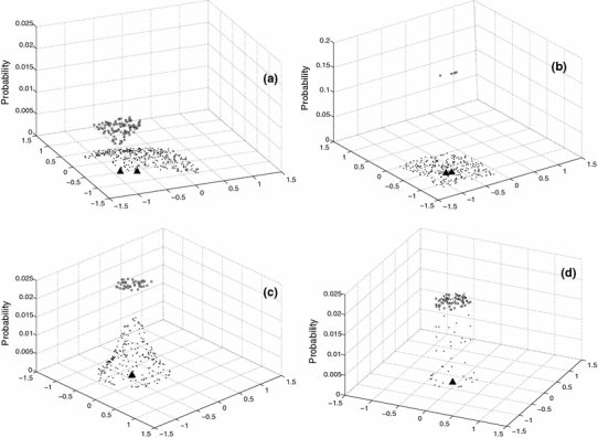
Probability distribution for the phases a, b, c, d for the fuzzy and hard subcluster of node 8 of cluster C1. The node position of subcluster 8 for every phase is shown in Fig. 7 by a square unfilled symbol. For phase b, much higher values for the probability-axis are necessary to note the data points of the hard cluster. Node—and hard centroid’s positions (filled triangles) are clearly separated in phases a and b but cannot be distinguished in phases c and d

For values of β < 5 in Fig. 6, E _nod ≈ 0, because the initial chain reduces to nearly a point. We see a first strong transition at point (a), where the nodes extend to a first configuration of the chain. This corresponds to a connection between few nodes that form at this value of β. Figure 7a shows nodes and hard centroids for this phase, Fig. 8a their standard deviations and Fig. 9a the probability distribution of node 8. The nodes accumulate in 4 points which should correspond to the optimal centroids of 4 fuzzy clusters. The chain is large and has a high E _nod, because it connects the different nodes in the 4 clusters multiple times. We have not connected the hard centroids, because they show a large dispersion. The standard deviations for the fuzzy clusters are much larger than the standard deviations for the hard clusters. The probability distribution of the fuzzy cluster 8 is largely extended and shows low probability values. Most data points have higher probabilities at the neighboring clusters, and the fuzzy cluster 8 is not well defined yet. The corresponding hard cluster is small, so that it has a much higher probability than the corresponding fuzzy cluster, and its centroid is different from the node position.

For increasing β, the nodes separate and the chain contracts. In phase (b), Fig. 7b, the nodes accumulate in 9 clusters, lowering in this way the interaction energy between nodes and data points. The hard centroids are now much nearer to the nodes, and Fig. 8b shows that the difference between the standard deviations get smaller. Fuzzy and hard cluster 8 are nearly nonexistent. In phase (c), the separation between the 20 nodes is nearly equidistant and covers the whole cluster. The hard centroids are approximately in the same position as the nodes and one expects that 20 fuzzy clusters exist. They are not well defined yet. This is seen in Fig. 8c, where the difference between the standard deviations is around 0.1. The stopping criterion (16) is nearly fulfilled. The probability distribution F _i8 in Fig. 9c defines much better the fuzzy cluster, but the range of the corresponding hard cluster is yet too small.

There is another marked change in E _nod between phase (c) and phase (d). In Fig. 7d, one notes that the nodes and hard centroids coincide. The standard deviations in Fig. 8d differ around 0.05. One node and its hard centroid have changed position such that the nodes cover better the area of the data points. The stopping criterion (16) is much better fulfilled for phase (d), and one could stop the annealing process. Figure 9d shows a well-defined fuzzy cluster 8, and the corresponding hard cluster has the same centroid and range. Finally, we note that the mean size σ_c of the clusters in phases a, b, c, and d are good approximations of the mean standard deviation of the fuzzy clusters.

For the second example, cluster C2, we see in Fig. 10 that the node interaction energy E _nod has a much clearer distinction of the different phases. This is a consequence of the three region of higher data point density in the inhomogeneous cluster which attracts more nodes. Figure 11 shows nodes and hard centroids for the 4 phases (a): , (b): , (c): and (d): , Figure 12 the standard deviations and the mean fuzzy cluster size σ_c for these phases and Fig. 13 the probability distributions of node 17. Node 17 was chosen because it is localized at a high density region.

Fig. 10.

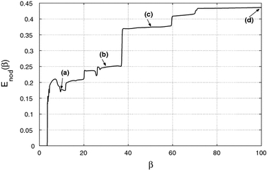
Node interaction energy E _nod as a function of β for cluster C2. The arrows indicate the phases a, b, c, d for data registrations

Fig. 11.

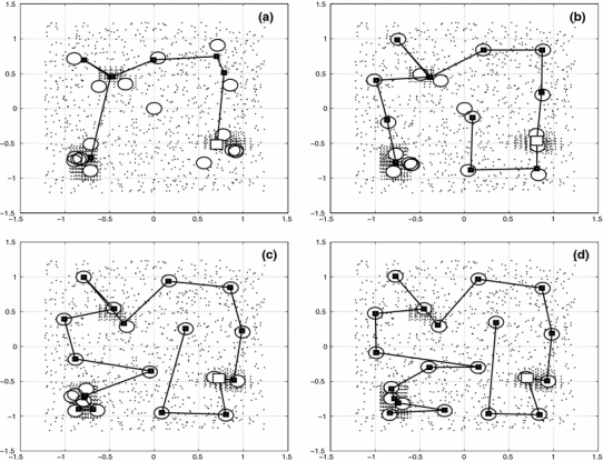
Data points, nodes, and hard centroids for the phases a, b, c, d of cluster C2. The node 17 is marked in every phase by a square unfilled symbol

Fig. 12.

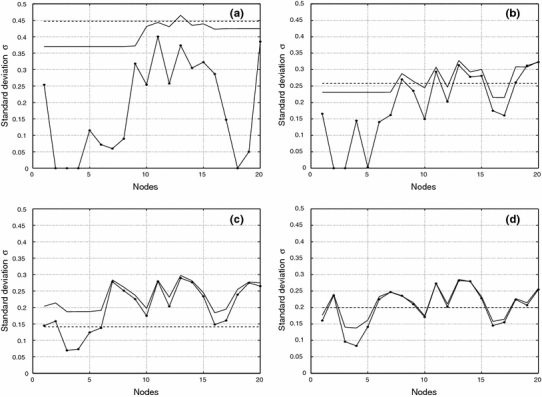
Standard deviations for fuzzy clusters, hard clusters, and the estimation σ_c for the phases a, b, c, d of cluster C2

Fig. 13.

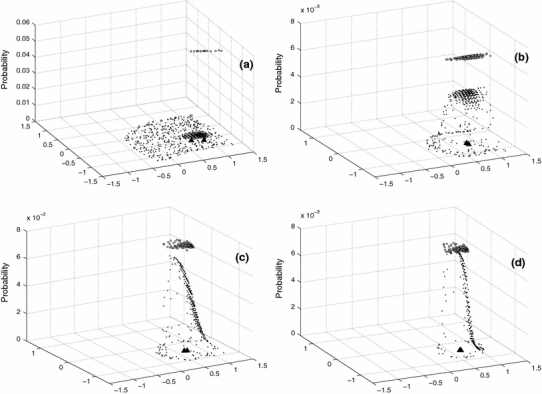
Probability distribution of the fuzzy and hard cluster for node 17 of cluster C2. Node 17 is marked in Fig. 11 by a square unfilled symbol. Node—and hard centroid’s position (filled triangles) are clearly separated in phase a but cannot be distinguished in the other phases

As in the homogeneous cluster C1, one notes in Fig. 11a that in cluster C2, after the first transition, all nodes are nearly in the same position of 4 subclusters, which should correspond to 4 fuzzy clusters formed in this phase, with the difference that some of the positions are now near the high density regions HDR. Hard centroids and nodes are different and in Fig. 12a one notes a large difference between the standard deviations. The standard deviation of the fuzzy clusters is constant for 3 group of nodes, which correspond to the nodes in the HDR. The estimation for the mean cluster size gives a larger value than the standard deviation for the fuzzy clusters. Figure 13a shows a low extended value for the fuzzy probability distribution and a small displaced hard distribution because there are neighboring nodes nearly at the same position and the fuzzy and hard cluster 17 are not well defined.

Figure 11b shows the next phase that gives a better formation of the chain of nodes and hard centroids with accumulation of nodes at the HDR. The hard centroids for the nodes which are at the HDR have larger deviations from their corresponding nodes. This seems to be a consequence of close proximity of the nodes in this region. Its fuzzy clusters are not well defined because their members are from low and high density regions. The problem may be solved by taking a larger number of nodes for the chain. This difference is seen too in the standard deviations in Fig. 12b for the nodes near or in the HDR. The mean cluster size approaches the fuzzy cluster standard deviation, and Fig. 13b shows a better formation of the probability distributions of node 17.

Phase c shows a nearly converged situation with 3 group of nodes in the HDR and a smaller difference between the nodes and hard centroids and between the standard deviations (Figs. 11c, 12c). The mean cluster size is a bit smaller than the mean values of the fuzzy and hard cluster standard deviations. The probability distributions (Fig. 13c) have nearly reached their optimal form and range.

In phase d (Fig. 11d), one finds a larger number of separate nodes with a node concentration in the HDR. Nodes and hard centroids are now in the same positions. The standard deviations of Fig. 12d are the same for the nodes outside the HDR and get smaller for nodes in the HDR. The mean cluster size gives a good mean value of the fuzzy cluster standard deviation. The probability distributions (Fig. 13d) have reached their best agreement.

For this case, one can stop the annealing process and determine the data points of the hard clusters and analyze its properties which should be in good accordance with the optimal fuzzy clusters for the given number of nodes.

We resume the main points of the last section.

• (i)As test case for the annealing process with ENA, we use a homogeneous cluster C1 and a nonhomogeneous cluster C2 with a chain of 20 nodes.
• (ii)The node interaction energy E _nod is zero for low β where all nodes are in the same position and from a certain β on shows phase transitions with a separation of the nodes. After sufficiently high values of β, all nodes are separated and the energy converges to a final constant value. For the nonhomogeneous cluster C2, the phase transitions are more pronounced and convergence requires a higher β-value.
• (iii)We show for 4 different values of the temperature parameter β, going from low values to sufficiently high values, the convergence of the chain of nodes and the standard deviation of the fuzzy clusters with the chain of hard centroids and the standard deviation of the hard clusters (16). In the nonhomogeneous cluster C2, one notes an accumulation of nodes in the high density regions. This may help to find inhomogeneous regions in n-dimensional data clouds.
• (iv)In order to get a feeling for the form and extension of the probability distribution for the fuzzy clusters F _ij and the corresponding distribution for the hard clusters H _ij (formulas 12 and 15), we show these distributions for a typical cluster. One notes that the extensions of F _ij and H _ij are minimal for the converged values of β.

Application to medical imaging

We use the algorithm formulated in chapter 2 and 3 in the analysis of medical imaging of X-ray computed tomography (CT) and positron emission tomography (PET) [9] of a patient with a lung carcinoma. The images were provided from the Hospital Universitario de la Pontificia Universidad Catolica de Chile, Grupo de Medicina Nuclear. The initial material consists of 435 CT and PET images of the whole body. For this analysis, we use only the slices that cover the part of the lung with the carcinoma. The carcinoma is localized between the slices 140 and 180 of the images. We apply the algorithm to a test series of 5 slices 140, 150, 160, 170, and 180.

Every CT image is given as a quadratic grid of pixels in Hounsfield units [10]. Its lower limit is −1,024, air has the value of −1,000. There is no upper limit. CT images give no clear information about the exact localization, form, and size of the carcinoma. The PET image is given in a smaller grid of pixels in standardized uptake values (SUV) [11]. Its lower limit is zero and there is no upper limit. They show a high pixel value (brightness) for the region with high biochemical activity, and carcinoma growing is one of these activities.

Figure 14 shows the CT image and the PET image of slice 160 of the test series. To use the same grid, we have extended the grid of the PET image to pixels, using the free software package ImageJ [12]. One notes clearly a small region of high biochemical activity in the PET image. The CT image shows well the structure of the lung in this slice, but it is not possible to localize precisely the place of the carcinoma.

Fig. 14.

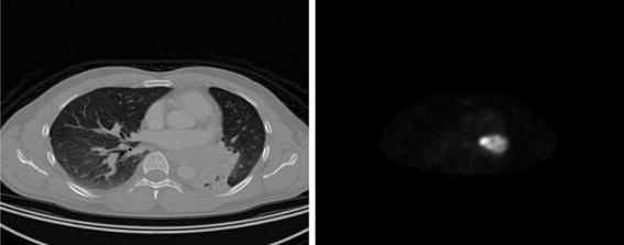
CT image (left) and PET image (right) for slice 160 of the test series

To localize its site, the CT and PET image for the same slice are superposed. For later comparison of all 5 slices and for applying the elastic net algorithm, we change the pixel values from the Hounsfield and SUV norm to the norm used for images with pixel values between 0 and 255. This is done using a linear scaling of the corresponding norm:

17

with the value of the pixel at grid point (i, j) in the Hounsfield (SUV) norm, its minimal and its maximal value of the 5 slices. p _ij gives the normalized value. The minimal value 0 corresponds to the lowest value of the 5 slices of the Hounsfiled (SUV) norm, and the maximal value 255 corresponds to the maximal value of the 5 slices.

For the superposition of the CT image with the PET image for the same slice, we use the following scaling:

18

with p ^ct _max and p ^ct _min the maximal and minimal CT pixel value of the same slice and p ^pet _max and p ^pet _min the maximal and minimal PET pixel value of the same slice. This guarantees that for and , . Figure 15 shows the superposed CT and PET images of Fig. 10. One notes the localization of the carcinoma as a bright spot at the middle of the image, but the precise size cannot be clearly seen.

Fig. 15.

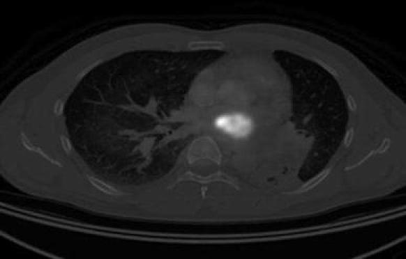
Superposed CT image and PET image for slice 160 of the test series

To get a better approximation for the size of the carcinoma in the slices, we search with the elastic net algorithm for patterns in the 5 two-dimensional clusters, formed by the pixel values of the CT and PET images for every slice. Every grid point (i, j) has two pixel values that are drawn in CT–PET diagram. The first column in Fig. 16 shows the 5 CT–PET cluster diagrams, where we have drawn only 800 homogeneously distributed data points of the total number of points. This dilution of the cluster points permits a better visualization of high- and low-density region in the cluster and the formation of possible patterns.

Fig. 16.

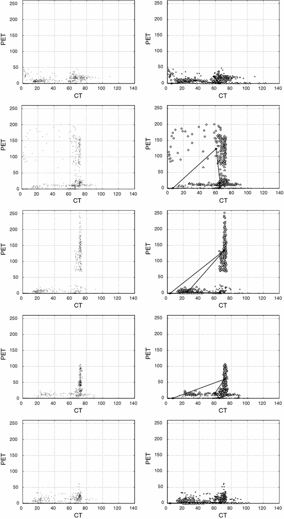
The 5 CT–PET cluster diagrams (first column), decomposition in 4 subclusters of the 5 CT–PET clusters together with the corresponding chain of 4 nodes (second column). The subclusters are marked with different symbols

In slice 140 one notes for all CT values low PET values with respect to its highest values of 255, only for small and intermediate CT values exist slightly higher PET values. This is different for the slices 150, 160, and 170 where exist, additionally to the low CT values a finger-like region in the middle of the CT region, which is separated from the lower region in slices 150 and 160 and goes to high PET values. It stems from the bright region in the PET image as a result of the carcinoma. In slice 160 exist the highest value for the finger. Here, we would expect the main localization of the carcinoma. In the final slice 180, the finger-like region is reduced and similar to slice 140. One can conclude that the CT–PET cluster diagrams give a more quantitative criterion to find the exact slice for which the carcinoma is brightest than the superposed CT–PET image.

We apply to the cluster diagrams the elastic net algorithm, using 4 nodes for a decomposition in 4 subclusters. The number 4 was chosen to have sufficient freedom in the formation of patterns, but no so large to take too much computer time. For the calculation, we used a laptop with Intel processor Core 2 Duo. For the slices 140 and 180, convergence was reached after 1,000 iterations which took about 20 min. For the slices with the finger-like cluster, 2,000 iterations were needed to reach convergence. Computer time can be considerably reduced if one paralyzes the elastic net algorithm.

The second column in Fig. 16 shows the 4 found subclusters together with the chain of nodes. To distinguish the 4 subclusters, we show only 200 homogeneously distributed data points per subcluster, marked with different symbols. In slice 140 and 180, the 4th subcluster has the highest PET values that are small and may come from other biochemical activity regions and not from the carcinoma. This changes strongly for slices 150, 160, and 170 where the chain of nodes is distorted for the second node which is the centroid of the subcluster 2, where the carcinoma is expected. The carcinoma region attracts the node 2 strongly.

We have converted the regions of the 4 subclusters into images and show in Fig. 17 the image of subcluster 4 for the slices 140 and 180 and subcluster 2 for slices 150, 160, and 170 which gives the image of the carcinoma. Finally, we calculated the complementary image, e.g. the image of the sum of all subclusters minus the subcluster 4 and 2, respectively, and show it in Fig. 17.

Fig. 17.

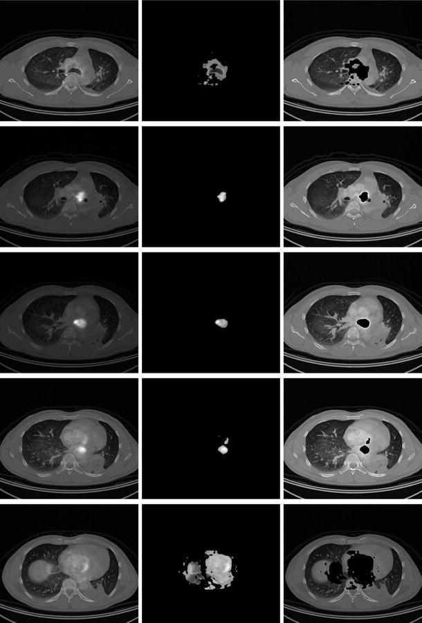
The 5 superposed CT–PET images (first column), images of subclusters 4 and 2 of the 5 CT–PET clusters, respectively (second column), images of the complementary images of the second column (third column)

The first column in Fig. 17 shows the superposed CT and PET images for the 5 slices, the second column the image of the subcluster 4 or 2 and the third column the complementary image of the second column. We see that slice 160 shows the maximal size of the carcinoma. The carcinoma images have been treated with ImageJ [12] to show edges. Figure 18 compares for slices 150, 160, and 170 the superposed images with the images of the edges of the complementary subcluster with the carcinoma. One notes that the elastic net algorithm gives a more quantitative result for the carcinoma site and size.

Fig. 18.

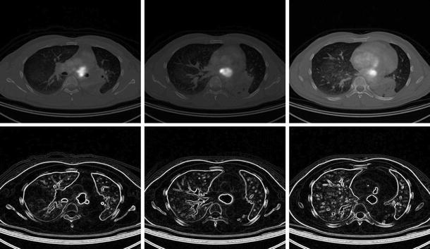
The superposed CT–PET images for slices 150, 160, and 170 (first row), images of the complementary clusters for slices 150, 160, and 170, treated with imageJ to show edges (second row)

Conclusions

We use a statistical mechanics formulation of the elastic net algorithm of Durbin–Willshaw for getting in a n-dimensional space a variable number of clusters which depend on a temperature parameter, or the inverse parameter β, of the annealing process. For a given number of nodes of the elastic chain, we find a value for β, for which the number of optimal fuzzy clusters are the same as the number of nodes and any further annealing with the new smaller optimal fuzzy clusters cannot be detected with the given number of nodes.

To determine the value of this β for which one can stop the annealing process, we define a hard centroid as the centroid of the cluster of nearest neighbors of every node, the hard cluster and find for the stopping condition that the hard centroid associated to every node must be the same as the node position and the same goes for their standard deviations. This means that the fuzzy clusters for this number of nodes are best approximated by this hard clusters with its known members which can be analyzed for their properties. An estimation of the mean cluster size as a function of β is given and shows a good approximation to the fuzzy cluster standard deviation. This means that for a given value of β, a mean cluster size is determined, but we do not know the minimal number of nodes that are necessary to give this cluster size at the stopping condition.

We illustrate the found relations by 2 two-dimensional clusters, one homogeneous cluster, where for the stopping condition the nodes are mostly equally spaced and cover the whole area, and a nonhomogeneous cluster with regions of different point density, where for the stopping condition the nodes accumulate at he high density regions. This second example shows that a similar situation in multivariate space can give clear information about smaller regions of different density.

Finally, we use the algorithm with the found convergence criteria to analyze medical CT–PET images that show lung cancer. The pixel values of the CT and PET images form two-dimensional clusters for every slice. The elastic net algorithm gives a more quantitative result for the localization and size of the carcinoma than the simple superposed CT–PET images.

References

- 1.Durbin R, Willshaw D. An analogue approach to the traveling salesman problem using an elastic net method. Nature. 1987;326:689–691. doi: 10.1038/326689a0. [DOI] [PubMed] [Google Scholar]
- 2.Rose K, Gurewitz E, Fox G. Statistical mechanics and phase transitions in clustering. Phys Rev Lett. 1990;65:945–948. doi: 10.1103/PhysRevLett.65.945. [DOI] [PubMed] [Google Scholar]
- 3.Yuille Alan. Generalized deformable models, statistical physics, and matching problems. J Neural Comput. 1990;2:1–24. doi: 10.1162/neco.1990.2.1.1. [DOI] [Google Scholar]
- 4.Duda R, Hart P, Stork D. Pattern classification. New York: Wiley; 2001. [Google Scholar]
- 5.Gorbunov S, Kisel I. Elastic net for standalone RICH ring finding. Proceedings—published in NIM A. 2006;559:139–142. doi: 10.1016/j.nima.2005.11.215. [DOI] [Google Scholar]
- 6.Salvini RL, de Carvalho LAV (2000) Elastic neural net algorithm for cluster analysis. Neural Networks, Proceedings, pp 191–195
- 7.Reichl LE. A modern course in statistical physics. New York: Wiley; 1998. [Google Scholar]
- 8.Ball K, Erman B, Dill K. The elastic net algorithm and protein structure prediction. J Comput Chem. 2002;23:77–83. doi: 10.1002/jcc.1158. [DOI] [PubMed] [Google Scholar]
- 9.Beyer T, Townsend DW, Brun T, et al. A combined PET/CT scanner for clinical oncology. J Nucl Med. 2000;41:1369–1379. [PubMed] [Google Scholar]
- 10.Hounsfield GN. Computerized transverse axial scanning (tomography): part 1. Description of system. Br J Radiol. 1973;46:1016–1022. doi: 10.1259/0007-1285-46-552-1016. [DOI] [PubMed] [Google Scholar]
- 11.Eckelman WC, Tatum JL, Kurdziel KA, Croft BY. Quantitative analysis of tumor biochemistry using PET and SPECT. Nucl Med Biol. 2000;27:633–635. doi: 10.1016/S0969-8051(00)00163-3. [DOI] [PubMed] [Google Scholar]
- 12.Collins TJ. ImageJ for microscopy. BioTechniques. 2007;43(1 Suppl):25–30. doi: 10.2144/000112517. [DOI] [PubMed] [Google Scholar]