Anisotropic material synthesis by capillary flow in a fluid stripe

Abstract

We present a simple bench-top technique to produce centimeter long concentration gradients in biomaterials incorporating soluble, material, and particle gradients. By patterning hydrophilic regions on a substrate, a stripe of prepolymer solution is held in place on a glass slide by a hydrophobic boundary. Adding a droplet to one end of this “pre-wet” stripe causes a rapid capillary flow that spreads the droplet along the stripe to generate a gradient in the relative concentrations of the droplet and pre-wet solutions. The gradient length and shape are controlled by the pre-wet and droplet volumes, stripe thickness, fluid viscosity and surface tension. Gradient biomaterials are produced by crosslinking gradients of prepolymer solutions. Demonstrated examples include a concentration gradient of cells encapsulated in three dimensions (3D) within a homogeneous biopolymer and a constant concentration of cells encapsulated in 3D within a biomaterial gradient exhibiting a gradient in cell spreading. The technique employs coated glass slides that may be purchased or custom made from tape and hydrophobic spray. The approach is accessible to virtually any researcher or student and should dramatically reduce the time required to synthesize a wide range of gradient biomaterials. Moreover, since the technique employs passive mechanisms it is ideal for remote or resource poor settings.

1. Introduction

Materials with gradients in chemical, mechanical, physical or biological properties are important tools for a wide range of applications including diagnostics, drug and material screening, and fundamental studies on cell behavior [1–11]. Hydrogels are commonly used for biological gradients since they mimic the extracellular matrix (ECM) and may be synthesized with tailored 3D microenvironments [7, 10–12] by manipulating their chemistry, crosslinking density and response to environmental stimuli [1, 4, 12–15]. Culturing cells within tailored 3D hydrogel scaffolds provides improved models for drug testing and microscale cell culture analogs of complex biological systems [12, 16–19]. Gradient hydrogels can spatially regulate cell behaviors such as migration [20–22], sprouting [23], angiogenesis [19, 24], attachment [25–27] and spreading/proliferation [21, 27–29]. Such gradient biomaterials enable a continuum of conditions to be tested simultaneously on a single biological sample.

A host of methods exist to create gradient biomaterials [4]. Many of these methods involve generating a gradient in the relative concentration of two prepolymer solutions and then crosslinking the mixture to form a gradient material. Techniques for generating prepolymer concentration gradients include the classic tree-like gradient generator [30], controlled mixing of input streams via a commercial gradient maker [22, 31], and convection in microchannels [6, 26, 27]. Hydrogel gradients are formed when concentration gradients of prepolymer solutions are crosslinked by chemicals, ultra-violet (UV) light, or temperature [1, 32]. By appropriate choice of input solutions and crosslinking method, hydrogels may be synthesized with gradients of soluble factors and mechanical properties, or which exhibit gradients in cell response [4]. Hydrogels have been produced with concentration gradients of toxins [33], drugs [34], chemoattractants [35], growth factors [20, 22, 23, 36–38], cell-adhesion ligands [21, 25, 27, 39], retroviruses [40], and with gradients in mechanical or physical properties such as pore size [30, 41–43], elastic modulus [30, 31], and matrix/fibril density [21, 23, 26]. Hydrogels exhibiting biological gradients are often formed from materials with complementary biological properties. Examples include a gelatin-hyaluronic acid (HA) gradient hydrogel exhibiting a gradient in cell attachment [26] and a chitosan-gelatin gradient hydrogel exhibiting a gradient in cell spreading [6]. Synthesizing hydrogels with photodegradable crosslinkers and photocleavable tethers can spatially and temporally tune peptide presentation and substrate modulus down to the micron scale for regulating dynamic cell-cell and cell-material interactions in 2D and 3D [44].

Recently, a simple gradient technique powered by capillarity and diffusion was developed to generate multi-centimeter long gradients of non-viscous solutions [34]. Using tape masks and hydrophobic spray, hydrophilic regions were patterned on glass slides (Fig. 1a,b) to hold fluid and direct flow without physical channel walls [45–48]. A stripe of fluid was pipetted onto the hydrophilic region (Fig. 1c). Adding a droplet to one end of this “pre-wet” stripe caused a rapid capillary flow that spread the droplet along the stripe to generate a gradient in the relative concentrations of the droplet and pre-wet solutions (Fig. 1d–f and Videos S1, S2). The gradient length and shape were controlled by the pre-wet and droplet volumes, stripe thickness, fluid viscosity and surface tension. The simple apparatus and the use of passive mechanisms make the technique ideal for remote or resource poor settings [49–52].

Figure 1.

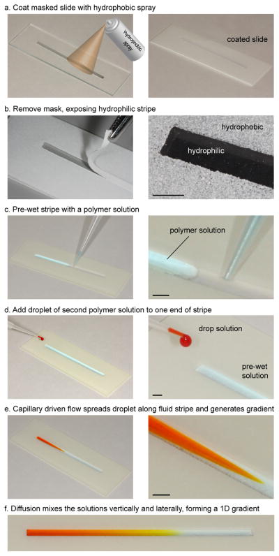
Device fabrication and experimental protocol. (a) Glass slide was masked and sprayed with a hydrophobic coating. (b) Coating dried and mask was removed, exposing a hydrophilic stripe surrounded by a hydrophobic boundary. (c) A prepolymer solution was pipetted onto stripe. (d) A droplet of a second prepolymer solution was added at one end of the stripe. (e) The increased capillary pressure due to the disturbance caused a ~10 cm s⁻¹ flow which rapidly spread the droplet solution along the stripe, forming a concentration gradient. (f) After diffusion mixed the solutions, a 1D polymer solution gradient was created.

Based on studies of gradient generation by convection (fluidic flow), a general rule is that faster flows generate longer gradients more rapidly [26]. Though our previous study on fluid stripe gradients dealt primarily with non-viscous solutions, the mathematical model we derived was not limited to low viscosity fluids and provided a scaling law for the flow speed u ~ (σ/μ)(V_d/V_w)(V_w/LW²)³(W/L), where W and L are the stripe width and length, V_w is the volume of the pre-wet solution, V_d is droplet volume, and μ and σ are the viscosity and surface tension of the fluid (in our model, we assumed the droplet and pre-wet fluids were the same for simplicity) [34]. The capillary flow speed is therefore proportional to the droplet volume V_d, surface tension, and to the square of the pre-wet volume, $V_w^2$, and is inversely proportional to viscosity. The fluid stripe depth was shown [34] to be proportional to V_w/LW, and hence for constant fluid depth, the speed is proportional to u ~ 1/W², i.e. faster speeds are expected for narrower fluid stripes. Here, we take advantage of these scaling laws to extend the method to more viscous solutions by using larger pre-wet and droplet volumes, and narrower stripes. Due to the complex dynamics of drop coalescence and the ensuing fluidic flow, abiding by these rules of thumb did not always yield the most linear gradients, though we have fully characterized the optimal parameters over a range of viscosities. Herein, the experimental protocol and physical picture of gradient generation on fluid stripes are outlined, including the dependence of the capillary flow speed on fluid viscosity and surface tension. The dependence of the concentration gradients on the fluid properties, stripe width, and protocol parameters are characterized to elucidate the optimal operational parameters for obtaining the most linear gradients. The technique is then used to create microsphere gradients in a variety of prepolymer solutions. Two biological gradients are also demonstrated, including a concentration gradient of cells encapsulated in 3D within a homogeneous biopolymer and a constant concentration of cells encapsulated in 3D within a biomaterial gradient exhibiting a gradient in cell spreading.

2. Materials and Methods

2.1 Materials

Hydrophobic WX2100 spray (Cytonix Corp., Beltsville, MD); pre-cleaned microscope glass slides (Thermo Fisher Scientific Inc., Waltham, MA); poly(ethylene glycol-diacrylate) (PEGDA, MW 2000 & 4000) and poly(ethylene glycol-dimethacrylate) (PEGDM, MW 1000) (Monomer-Polymer & Dajac Labs, Trevose, PA); photoinitiator (PI) 2-hydroxy-1-[4-(hydroxyethoxy)phenyl]-2-methyl-l-propanone (Irgacure D2959, Ciba Specialty Chemicals Inc., Florham Park, NJ); gelatin, heparin sodium salt (avg. MW 18 kDa), methacrylic anhydride, 3-(trimethoxysilyl) propyl methacrylate, (Sigma-Aldrich Inc., St. Louis, MO); sodium hyaluronate (avg. MW 53 kDa, Lifecore Biomedical Inc., Chaska, MN); green fluorescent polymer 10 μm microspheres (1 wt% solids, Duke Scientific Corp., Palo Alto, CA); Live/Dead^® and phalloidin (Alexa Fluor 594) stains (Invitrogen Corp., Carlsbad, CA); 4,6-Diamidino-2-phenylindole (DAPI, Vector Laboratories Inc., Burlingame, CA). NIH-3T3 cells were cultured in Dulbecco’s modi ed Eagle medium (DMEM, Invitrogen Corp., Carlsbad, CA) supplemented with 10%fetal bovine serum and 1% penicillin streptomycin (Invitrogen Corp., Carlsbad, CA) in a 5% CO₂, 37 °C incubator. Gelatin, HA, and heparin were methacrylated by standard chemical procedures to produce gelatin methacrylate (GelMA) [53], hyaluronic acid methacrylate (HAMA) [54], and heparin methacrylate (HepMA) [55]. All other reagents and tissue culture components were purchased from Sigma-Aldrich Inc. (St. Louis, MO) unless otherwise noted.

2.2 Coated slide fabrication

The coated slides were produced with minor modifications to a previous protocol [34]. Glass slides were masked with rectangular strips of MacTac 8300 cut by a Graphtec cutting plotter CE5000-60 (Graphtec America Inc., Santa Ana, CA). Hydrophobic spray (WX2100) was applied and allowed to dry for 2 days. The MacTac masks were then carefully removed. Slides with custom coated hydrophobic regions may be purchased directly from the manufacturer (e.g. Cel-Line Brand Specialty Printed Slides and Multi-Well Slides with custom coatings from Thermo Scientific’s Slides and Specialty Glass division, Portsmouth, NH).

2.3 Gradient protocol

Following a previous protocol for non-viscous solutions [34], a fluid stripe was formed by pipetting a given “pre-wet volume” of one solution along a plasma-treated hydrophilic stripe of a coated slide (Fig. 1c). Plasma cleaning had no noticeable effect on the hydrophobic region. A drop of a second solution containing the salient molecules or particles was added by first secreting the full droplet from a pipette tip and suspending it ~1 mm above one end of the pre-wet stripe (Fig. 1d and Videos S1, S2). The angle between the center axis of the pipette and the centerline of the stripe was kept less than 20°, though greater angles did not appreciably change the shape of the gradient. With one swift, short, gentle shake of the pipette, the drop detached from the pipette tip and fell to the pre-wet stripe, generating a capillary flow and a spatial gradient along the stripe in the relative concentrations of the droplet and pre-wet solutions (Fig. 1e). Alternate methods of drop addition such as quickly touching the drop to the pre-wet stripe gave similar results. Following droplet addition, the gradient fluid stripe was allowed to stand for a prescribed amount of time while diffusive mixing smoothed the gradient profile vertically and laterally (Fig. 1f). The device was kept in a humid Petri dish (with wet towel) to avoid evaporation. All prepolymer solution gradients were formed at 25 °C. Tilting or agitating the device could induce fluid motion in the fluid stripe, distorting the gradient. Device and fluid motion were minimized by performing the gradient protocol where it was to be imaged or stabilized, for example, on the microscope stage or within the fluorescent camera or UV lamp enclosure.

2.4 Flow speed experiments

The gradient protocol was carried out with pre-wet solutions containing 1X Dulbecco’s Phosphate Buffered Saline (DPBS) solution with 5%, 20% and 40% (w/v) PEGDM 1000. Droplets of Trypan blue solution containing the same % PEG as the pre-wet solution were pipetted onto one end of the fluid stripe. In some cases, Tween-20 was added to both the droplet and pre-wet solutions at the same concentration, either 0.1% or 1% (w/v). Subsequent fluid motion was recorded by digital camera at 60 frames per second (fps) and the dye tip position was measured in successive frames with Matlab. For the still images shown in Figure 2 and for Videos S1 and S2, a high-definition (HD) camcorder was used with a frame rate of 30 fps. Each experiment was repeated three times. The viscosities and surface tensions of the various concentrations of PEGDM 1000 are listed in Tables S1 and S2.

Figure 2.

Physics of soluble gradient production on a fluid stripe. (a) Frames captured from video illustrate the droplet coalescence and ensuing capillary-driven flow. The flow is initially of order ~10 cm s⁻¹, depending on the viscosity, and slows to ~1 cm s⁻¹ by 50–200 ms. Measured speeds for different concentrations of PEGDM 1000 are plotted in dimensionless coordinates and compared to a previously derived theoretical model [34]. Experiments were repeated at least three times and the standard deviation was less than the symbol size except where noted by error bars. (b,c) Molecular diffusion smoothes the vertical and lateral composition of the prepolymer solution stripe. The vertical and lateral diffusive mixing of (b) the small molecule fluorescein is virtually complete within 10 minutes, producing a smooth 1D gradient, and that of (c), the large molecule 70 kDa FITC-dextran is still active after 19 mins.

2.5 Fluorescence imaging

Fluorescence images were captured with a Kodak Gel Logic 100 Imaging System with optimal exposure times and zoom. The fluorescence intensity along the stripe was quantified by ImageJ and Matlab.

2.6 Concentration gradients in stripes of prepolymer solutions

The gradient protocol was carried out by pre-wetting the stripe with a given prepolymer solution and adding a drop of the same or another prepolymer solution. In some cases, for visualization and quantification, 0.1% (w/v) fluorescein or 0.1% (w/v) fluorescein isothiocyanate-dextran (FITC-dextran, MW 70 kDa) were added to the droplet solution and gradients were quantified by fluorescence imaging. Polymer solutions included: 5, 10, 20, 30, 40% (w/v) PEGDM 1000, PEGDA 2000 or PEGDA 4000 dissolved in DPBS; 3% or 5% (w/v) GelMA dissolved in DPBS; 1% (w/v) HAMA dissolved in DPBS, 2% (w/v) HepMA dissolved in DPBS. The viscosities and surface tensions of these polymer solutions are listed in Tables S1 and S2.

2.7 Microsphere gradients in stripes of prepolymer solutions

The gradient protocol was carried out by pre-wetting the stripe with a given prepolymer solution and then adding a drop of the same solution plus 10 μm diameter green fluorescent microspheres, diluted 20 times from the stock solutions. Images were captured along the length of the stripe with an inverted fluorescence microscope (TE-2000-U, Nikon, Melville, NY) with 2X and 10X objectives, and quantified with Matlab. The 10X images were taken every 0.5 cm along the stripe, starting at approximately 0.25 cm from one end of the stripe.

2.8 Confocal Laser Scanning Microscopy (CLSM)

The distribution of 10 μm FITC fluorescent microspheres in a gradient was quantified by Confocal Laser Scanning Microscopy (CLSM, Leica TCS SP5 II, Bannockburn, IL) with a 10X objective (HCX PL APO CS 10X 0.4 DRY) at 2.5 μm vertical z-intervals. FITC fluorescence was detected upon excitation at 495 nm through a cut-off dichroic mirror and an emission band-pass filter of 505–540 nm. The prepolymer gradient was formed using our gradient protocol with a 20 μl pre-wet solution of 5% PEGDM 1000 and a 10 μl drop of 10 μm microspheres (at 20X dilution), 0.5% PI (w/v), and 5% (w/v) PEGDM 1000 in DPBS. The gradient was allowed to stand for 1 minute following droplet addition, and was then photocrosslinked by 90 s exposure to UV light (wavelength 360–480 nm, power 6.9 mW cm⁻²).

2.9 Cell concentration gradient in a hydrogel scaffold

The gradient protocol was followed with a 15 μl pre-wet solution of 5% (w/v) GelMA and 0.5% PI (w/v) in DPBS and a 5 μl drop of 5% (w/v) GelMA and 0.5% PI (w/v) in DPBS containing NIH-3T3 cells (5×10⁶ cells/ml). 1 min after droplet addition, the prepolymer stripe was photocrosslinked by 30 s exposure to UV light (wavelength 360–480 nm, power 6.9 mW cm⁻²), placed in DMEM, and incubated at 37 °C for 4 hours. The stripe was then stained with a Live/Dead^® assay and imaged with fluorescence microscope. The quantification protocols were the same as for the microsphere gradients.

2.10 Cell spreading gradient in a gradient hydrogel

The gradient protocol was followed with a 15 μl pre-wet solution containing NIH-3T3 cells (5×10⁶ cells/ml), 0.5% (w/v) PI and 1% (w/v) HAMA in DPBS and a 5 μl drop of 0.5% (w/v) PI and 5% (w/v) GelMA in DPBS. The gradient prepolymer solution was allowed to stand for 1 min, and was then photocrosslinked by 15 s exposure to UV light (wavelength 360–480 nm, power 6.9 mW cm⁻²). The device was placed in DMEM and incubated at 37 °C for 1 day. To visualize cell spreading, the gradient hydrogel was fixed with 4% paraformaldehyde and stained with phalloidin and DAPI according to manufacturer protocols to visualize F-actin filaments and cell nuclei, respectively. Overlapping 2X phase images and 10X (not shown) and 20X phase and fluorescence images were captured by inverted fluorescence microscope. Cell counts were extracted from 20X phase images of the stripe captured at day 0 (i.e. following crosslinking) using ImageJ and Matlab.

2.11 Data analysis

Statistical significance was determined by balanced one- and two-way analysis of variance (ANOVA). For all statistical tests, the level of significance was set at p < 0.05. For the gradient profiles in Figure 3(a–i), the relative intensity profile from each trial was first averaged over 0.5 cm intervals to produce a discrete data series of 10 relative intensities equally spaced along the stripe (Fig. S1). A p-value was calculated from each pair of data series by a balanced two-way ANOVA test in Matlab (Table S3). For the microsphere gradients in Figure 4c, the p-values calculated from each pair of data series by a balanced two-way ANOVA in Matlab test are listed in Table S4.

Figure 3.

Concentration gradients in various prepolymer solutions. (a) Gradients in PEG 1000, 4000 and GelMA at different polymer concentrations for fixed pre-wet volume V_w = 20 μl and drop volume V_d = 10 μl. Gradient in PBS (V_w = 15 μl, V_d = 7.5 μl) plotted for comparison. (b) Polymer gradient profiles made from different pairs of droplet / pre-wet solutions (2% HepMA / 3% GelMA; 2% HepMA / 1% HAMA; 5% / 40% PEGDM 1000; 3% GelMA / 40% PEG 1000; 1% HAMA / 3% GelMA). Characterization of gradient profiles based on effect of: (c) volume ratio V_d/V_w with V_w = 20 μl (20% PEG) and V_w = 24 μl (40% PEG); (d) stripe width W with V_w/W = 10 μl mm⁻¹, V_d/V_w = 1/2; (e) pre-wet volume V_w with V_d/V_w = 1/2; (f) surface tension, altered artificially by adding Tween surfactant in equal % to both the pre-wet and droplet solutions, with V_w = 20 μl, V_d = 10 μl. Gradient profiles grouped into three classes according to shape: (g) gradients in low viscosity solutions, 0.9 to 3.4 cSt (3% GelMA’s viscosity could be moderately higher), had relatively monotonic and linear profiles; (h) gradients in intermediate viscosity solutions, 1.7 to 13.2 cSt, each had a large characteristic peak in the region of drop coalescence; (i) gradients in high viscosity solutions, 19.4 to 50 cSt, had a region of approximately constant concentration followed by a steep linear decrease to zero. (j) Effect of user and repetition, for V_w = 20 μl, V_d = 10 μl. In cases (a–i), the droplet consisted of the pre-wet solution plus 0.1% fluorescein for visualization. In all cases, the fluorescent intensity profiles shown were taken 11 mins after droplet addition, when they had converged to their steady state following vertical and lateral diffusive mixing.

Figure 4.

Microsphere gradients in prepolymer solutions. (a) Fluorescence images of a 10 μm microsphere gradient in 3% GelMA. 2X microscope images indicate the overall gradient profile, while the 10X zooms below indicate the 3D positioning of the particles (microspheres out of focus were above or below the focal plane). (b) Inverted confocal microscope images quantify the vertical distribution of particles near the beginning, middle, and tip of a 10 μm microsphere gradient in 5% PEGDM 1000. Following generation of the particle gradient, the prepolymer stripe was crosslinked to fix the particles in their respective vertical positions. Histograms summarize the vertical positioning of the particles in the central regions of the confocal images (defined in Fig. S4) relative to the position of the lowest particle detected. (c) 10 μm microsphere gradients were produced in various prepolymer and other solutions and then quantified by fluorescence microscope. Bar charts summarize the normalized and laterally averaged microsphere counts along each gradient. Error bars indicate the standard deviation over three repetitions. The observed variation was due to the relatively low microsphere concentration; there was not a statistically significant difference between most of the data series. Scale bars: (a) 100 μm and (b) 200 μm, except where noted.

3. Results and discussion

3.1 Gradient generation by capillary flow on a fluid stripe

The experimental technique follows a previous method for non-viscous solutions [34], and is outlined in Figure 1. Using masks and hydrophobic spray, glass slides were patterned with rectangular hydrophilic stripes surrounded by hydrophobic coatings (Fig. 1a,b). The stripes were pre-wet with a prepolymer solution, which wet the glass and was held in place by the hydrophobic boundary (Fig. 1c). Stability and other properties of fluid stripes have been reviewed previously [34, 56, 57]. Adding a droplet of a second solution to one end of the stripe caused a local increase in the capillary pressure, which drove the flow and spread the droplet solution along the fluid stripe (Fig. 1d and Videos S1, S2). The resulting gradient was subsequently smoothed vertically and laterally by diffusive mixing (Fig. 1f).

The capillary-driven flow on the fluid stripe was characterized by measuring the position of the tip of a droplet of dye spreading on a pre-wet fluid stripe, for prepolymer solutions of different viscosities and surface tensions. Videos S1 and S2 demonstrate gradient generation on stripes of 5% and 40% PEG 1000, respectively. The flow speed on the 40% stripe is noticeably lower than on the 5% stripe due to the larger prepolymer concentration and viscosity (confirmed in Fig. S3a). The measurements approximately collapsed by plotting them in terms of the previously derived [34] characteristic time and length scales, $t_0=2\mu L^5{W}^5{V}_d^2/(81\sigma V_w^5)$ and x₀ = LV_d/V_w, respectively, where Wand L are the stripe width and length, V_w is the volume of the pre-wet solution, V_d is droplet volume, and μ and σ are the viscosity and surface tension of the drop and pre-wet solutions listed in Tables S1 and S2, respectively (Fig. 2a and Fig. S2). In our speed experiments, the drop and pre-wet solutions were the same, except for the Trypan blue dye, which we assumed did not appreciably alter the viscosity or surface tension. Identifying the precise time of flow initiation was complicated by coalescence and could have occurred during frames; the time of the first frame of each data set was set arbitrarily to t = 0.005 s, half of that chosen in a previous study [34], since the frame rate used here was higher. The three theoretical curves plotted in Fig. 2a were derived previously [34] for different forms of the disturbance depth H = h₀, (h₁+h₀)/2, h₁, where h₀ is the depth of the pre-wet solution and h₁ the depth of the disturbance. The approximate data collapse in Fig. 2a and Fig. S2 onto our theoretical model re-confirms the speed scaling law listed above. In particular, as the polymer concentration in an aqueous solution increases, the viscosity of the solution increases and the flow speed decreases (Videos S1, S2 and Fig. S3a). To test the effect of surface tension on the flow speed, we artificially lowered the surface tension of a 20% PEG solution and measured proportionally lower flow speeds (Fig. S3b).

Once the capillary flow on the fluid stripe subsided, the contents of the stripe mixed laterally and vertically due to molecular diffusion. The time for a solute to diffuse a distance L is L²/(π²D), where D is the molecular diffusivity. For example, fluorescein diffusing through buffer solution has a diffusivity of D = 2.7×10⁻⁶ cm² s⁻¹ [58], and thus requires approximately 6 s and 10 min to diffuse 100 μm and 1 mm, respectively, the order of magnitudes of the depth and width of the fluid stripe. The diffusivity of a given molecule in a prepolymer solution decreases with the volume fraction of the polymer [59]. Rather than measure the diffusivity and calculate the necessary diffusion time, the partial opacity of our prepolymer solutions to the light emitted by fluorescein and FITC offered a direct measure of the degree of cross-sectional uniformity of their concentration gradients. The diffusive mixing of fluorescein in 20% PEG 1000 (Fig. 2b) and for 70 kDa FITC-dextran in 3% GelMA (Fig. 2c) were captured by fluorescence camera. As the fluorescein in the droplet solution diffused laterally across the stripe and vertically into the pre-wet solution below, the centerline intensity decreased. The convergence of the centerline intensity profile in Fig. 2b indicated that the vertical and lateral mixing were complete in approximately 10 mins; the lack thereof in Fig. 2c demonstrated that the larger dextran molecules diffused more slowly and the cross-sectional mixing was still occurring after 19 mins. For cases where gradient prepolymer solutions are crosslinked to form gradient materials, the amount of diffusion time may be adjusted to control the degree of cross-sectional uniformity of the gradient material. Lastly, we note that due to the cylindrical shape of the fluid stripe, the fluid depth and fluorescent intensity were less at the edges than at the center, even when the lateral concentration was uniform [34].

3.2 Characterization of prepolymer solution gradients in a fluid stripe

A myriad of concentration gradients were prepared with our fluid stripe platform for a wide range of polymers and concentrations. In addition, the effects of protocol parameters (droplet, pre-wet volumes), fluid properties (viscosity, surface tension), and device design (stripe width) were probed to determine experimentally the conditions resulting in the most linear gradients. The results are summarized in Figure 3. The discussion will first focus on gradients of different polymer types and concentrations, followed by a discussion of the effects of protocol parameters, device design, fluid properties, and repeatability. Lastly, a heuristic argument is outlined in an attempt to rationalize the observed gradient profile shapes. For a consistent comparison, all gradients were visualized and quantified by adding fluorescein to the droplet solution. Fluorescence images were captured at two minute intervals starting 1 min after droplet addition. Centerline intensity profiles were extracted from each fluorescence image, and in all cases tested, had converged by 11 mins after droplet addition. The converged centerline intensity profiles at t = 11 min are plotted in Figure 3 and grouped with respect to the particular effect tested.

Dye concentration gradients in homogeneous prepolymer solutions were generated by pre-wetting the stripe and adding a droplet of the same solution plus dye to the pre-wet stripe (Fig. 3a). Gradients in prepolymer solutions of different polymers (PEG 1000 and 4000, GelMA) and concentrations were produced. In general, the gradient profiles became more nonlinear as the prepolymer concentration, and hence viscosity, increased. However, for PEG 1000, despite profiles becoming more nonlinear as the concentration increased from 0% to 20% (p < 0.05), the profiles became more linear for higher concentrations. For example, there was a statistically insignificant difference between the 5% and 40% profiles. For PEG 4000, the difference between the 0–10% profiles was not statistically significant, but higher concentrations led to a statistically significant increase in profile nonlinearity. These profile changes illustrated the complexities of the droplet coalescence and ensuing capillary flow and their dependence on viscosity and molecular weight.

Gradients in the relative concentrations of polymer solutions containing either different polymers or different concentrations of the same polymer are shown in Figure 3b. Concentration gradients were created with droplets and pre-wet stripes containing, respectively: 2% HepMA and 3% GelMA; 2% HepMA and 1% HAMA; 5% and 40% PEGDM 1000; 3% GelMA and 40% PEGDM 1000; 1% HAMA and 3% GelMA. Relatively linear gradients were obtained for the 5% to 40% PEG and the GelMA-PEG gradients; more nonlinear gradients were obtained for the others (p < 0.05).

Increasing the droplet to pre-wet volume ratio, V_d/V_w, while keeping other parameters constant, extended the gradient profile further along the stripe (Fig. 3c). Our previous study showed that in water or buffer solution, the droplet solution spread over a distance largely determined by the volume ratio [34]. The extent of the gradient profiles increased smoothly with increasing volume ratio for 20% PEG 1000, and more irregularly so for 40% PEG 1000. For both polymers, linear 2 cm gradients were observed for the smaller volume ratios tested. For 20% PEG 1000, the linear portion of the gradients became shorter with increased volume ratios. For 40% PEG 1000, the profiles became less linear with increased volume ratio, though at V_d/V_w = 3/4, relatively linear 3 cm gradients were observed. The pair-wise differences between profiles were statistically significant, except for volume ratio pairs of (1/2, 1/4) and (1/2, 1/3).

Parameters such as stripe width, pre-wet volume, and surface tension, as well as the person performing the experiments, had less significant effects on the gradient profiles. In each case that follows, the particular parameter was varied while the others were held constant. Changes to stripe width in the range of 1 to 2 mm seemed to cause only minor changes in the gradient profiles, at least for 20% and 40% PEG 1000 (Fig. 3d). Stripe widths were tested by fixing the volume ratio at V_d/V_w = 1/2 and the pre-wet to width ratio at V_w/W = 10 μl/mm. The differences between gradient profiles on the 1.5 mm and 2 mm stripes were not statistically significant; the 1 mm stripes had more linear gradients (p < 0.05). In practice, stripe width would likely be chosen based on other factors, such as ease of use. Altering the pre-wet volume had only a minor effect for 20% PEG 1000, while the effect was more irregular for 40% PEG 1000 (Fig. 3e). The gradient profiles corresponding to pre-wet volumes 15 μl and 20 μl were not statistically significant. More linear gradients were obtained for the highest pre-wet volume, 24 μl (p < 0.05). As noted in our previous study [34], if the pre-wet volume was too large, the capillary-driven flow was insufficiently damped and the disturbance was reflected when it reached the end of the stripe, distorting the concentration gradient. The effect of surface tension on gradient profile shape was measured by adding surfactant to both the droplet and pre-wet stripe to artificially lower their surface tension (Fig. 3f). Adding surfactant decreased the surface tension and the flow speed (Fig. S2), but made no statistically significant difference to the gradient profiles. The effect of user bias and the variability associated with repetition was measured in Figure 3j; only minor differences were noted between trials and users.

To provide a certain order to the various gradient profile shapes observed, we grouped gradient profiles with similar shape (Fig. 3g–i). The viscosities of the solutions in each group (Table S1) also fell into three classes, supporting the premise that gradient profile morphology was largely determined by viscosity. Solutions with low viscosity (0.9 to 3.4 cSt, except 3% GelMA, whose viscosity could be moderately higher) had relatively monotonic and linear gradient profiles (Fig. 3g). In the intermediate viscosity range (1.7 to 13.2 cSt), gradient profiles had a large characteristic peak in the region of drop coalescence (Fig. 3h). In the high viscosity range (19.4 to 50 cSt), gradient profiles consisted of a region of approximately constant concentration followed by a relatively steep linear decrease to zero (Fig. 3i). In this latter class, the gradients were approximately 1 cm long, except for 1% HAMA, which had the highest viscosity (~50 cSt) and whose gradient was less than 0.5 cm long. For a given prepolymer solution, the viscosity values reported in the literature could vary by over 100%, indicative of the sample to sample variation. This variation could be partly to blame for the apparent overlap of the viscosity ranges for the first two gradient morphology classes. Also, our simple classification ignores the differences between prepolymer solutions such as the degree of non-Newtonian behavior. In Fig. 3g–i, we limited the profiles plotted to those with a volume ratio of V_d/V_w = 1/2 and a stripe width of W = 2 mm.

Despite the complexity of droplet coalescence and the ensuing capillary flow, we postulate a simple rationale to explain the different gradient profile shapes observed for solutions of low and high viscosity. When a droplet coalesces with the pre-wet solution, it sinks into the stripe and also spreads along the stripe. In order to sink into the stripe, the underlying fluid must be displaced, since the fluids employed are incompressible. Viscosity retards this fluid displacement, so more drops coalescing with more viscous pre-wet solutions sink less. If the droplet solution remains in the upper portions of the stripe, it only experiences the upper range of fluid velocities, since a good assumption is that the velocity decreases from its maximum at the free surface to zero at the substrate. Since the gradients reported here were generated by convective mixing, in which a concentration profile is distorted by exposure to a range of velocities, the convective mixing is less for droplets exposed only to the upper range of velocities. Hence, neglecting other factors such as non-Newtonian effects, longer and more linear gradients are obtained for less viscous solutions, a rule of thumb supported by comparing the gradient profiles in Figs. 3g and 3i.

Our gradient characterization relied on adding fluorescent dye to the drop solutions for rapid visualization. We note that for drops and pre-wet volumes containing different prepolymer solutions, complete cross-sectional mixing may take much longer than the 11 mins required by the fluorescein dye, especially for high molecular weight polymers and concentrated solutions. If desired, a tagged prepolymer solution could be used to assess uniformity. Once protocol parameters are selected for a particular application, the gradient biomaterial may then be characterized for its gradient biological, chemical, mechanical, and physical properties. Two classes of examples are considered next.

3.3 Microsphere gradients in prepolymer solutions

Concentration gradients of 10 μm microspheres were produced in various prepolymer solutions by adding a droplet containing microspheres to a pre-wet stripe (Fig. 4). The microspheres settled during and following the capillary flow. The settling speed of 10 μm diameter microspheres (density 1.05 g ml⁻¹) is 3 μm s⁻¹ in distilled water [26] and varies inversely with viscosity. Thus, in 5% GelMA, which is approximately 10 times more viscous than water at 25 °C, the microspheres would settle ten times more slowly. Also, the settling speed is proportional to the square of particle diameter, so that smaller particles would remain suspended in 3D even longer. Crosslinking enables the microsphere positions to be fixed in 3D within a gel scaffold; adjusting the time between droplet addition and crosslinking alters their 3D positioning. Fluorescence images of a concentration gradient of 10 μm microspheres in 3% GelMA are shown in Fig. 4a. The stitched 2X images give a top-down view of the overall gradient shape; the 10X zooms illustrate the change in microsphere concentration along the stripe and also the variation in vertical 3D positioning (microspheres out of focus were above or below the focal plane). The 3D distribution of 10 μm microspheres in crosslinked 5% PEG 1000 is visualized by inverted confocal microscopy in Fig. 4b. Inset bar charts show that the microspheres near the region of drop coalescence sunk lower and were distributed more vertically than those further down the stripe. Microsphere concentration gradients were generated in a variety of prepolymer and other solutions and quantified by the relative concentration (Fig. 4c). Here, the relative concentration refers to the number of microspheres in a 10X image centered on the stripe centerline, divided by the maximum count along the stripe. In general, the gradients in relative concentration were more linear for the less viscous solutions. The observed variation, quantified by error bars, was due to the relatively low microsphere concentration; the pair-wise differences between many of the series were not statistically significant.

3.4 Biological gradients

The gradient fluid stripe technique was used to generate two types of biological gradients. The first was a cell concentration gradient in 5% GelMA formed by adding a droplet of 5% GelMA solution containing cells to a pre-wet stripe of 5% GelMA solution not containing cells. Photocrosslinking the polymer stripe encapsulated the cells in 3D. Live/Dead^® staining indicated that 92 ± 4% of the cells were live following this procedure (Fig. 5a). The concentration gradient was visualized by fluorescence and phase microscope images and quantified by cell counts along the stripe (Fig. 5a). The 10X fluorescence images indicated that the cells were distributed vertically as well as horizontally; cells not in focus were above or below the focal plane.

Figure 5.

Biological gradients. (a) A cell concentration gradient was produced when a droplet of 5% GelMA containing cells was added to a pre-wet 5% GelMA fluid stripe. The gradient was visualized by Live/Dead^® staining, overlapping 2X fluorescence microscope images and 10X phase and fluorescence zooms taken near the centerline along the gradient. Laterally averaged live/dead cell counts decreased along the gradient. * denotes p < 0.006. (b) Cell spreading gradient along a 5% GelMA 1% HAMA gradient biomaterial visualized by overlapping 2X phase microscope images and 20X phase and fluorescence images of the cells stained for F-actin (phalloidin) with a nucleic counterstaining (DAPI). As expected, cells in the GelMA rich regions spread well, while those in the HA-rich regions did not spread. Comparing cell counts on gradient stripes (drops added) and on control pre-wet only stripes (no drops added, Fig. S5b) demonstrates that the cell concentration remained nearly constant in the material gradient region. In each spatial interval, p-values between data series were larger than 0.05 except in the cell washout region where p < 2×10⁻⁵ (**). In (a,b), error bars indicate the standard deviation over three repetitions. Scale bars: (a) 200 μm and (b) 100 μm, except where noted.

A second biological gradient was formed by adding a droplet of 5% GelMA to a pre-wet stripe of 1% HAMA solution containing NIH-3T3 cells. The resulting gradient prepolymer solution was photocrosslinked 1 minute after droplet addition, encapsulating the cells in 3D. Following 1 day of culturing, a cell spreading gradient was observed along the stripe (Fig. 5b), and may be compared to the control cases of cells cultured in pure 5% GelMA [53], where most cells spread, and pure 1% HAMA (right end of stripe, and Fig. S5c), where cells did not spread. The sharp tip of the spreading gradient is indicative of the early form of the gradient morphology noted in Fig. 1e. Waiting longer times following droplet addition would allow additional time for molecular diffusion to mix the GelMA and HAMA solutions and soften the transition in the tip region. An additional attractive feature of our technique is the fact that by adding the cells to the pre-wet solution, and not the droplet, the cell concentration was relatively constant (similar to the pre-wet only control) everywhere along the gradient stripe except near the region of drop coalescence (Figs. 5b and S5a). In particular, the cell concentration in the high GelMA, gradient GelMA-HAMA, and HAMA only region was roughly constant, allowing fair comparisons between the observed cell behaviors in each region. The coalescence region where cells were washed aside or downstream by the flow was confined to the first 1 cm of the 5 cm stripe.

3.5 Additional remarks and future directions

We have presented a simple technique for generating centimeter scale concentration gradients in fluidic stripes of prepolymer solution held on the surface of glass slides. By crosslinking the resulting gradient prepolymer solutions, composite polymers were produced containing concentration gradients in soluble factors, cells, and microspheres, and gradients in biological properties. The polymers used in this study were chosen for their relevance to biomedical engineering. Provided the viscosity of a given prepolymer solution is sufficiently low (in this study, we considered those below 50 cSt), the platform should be able to generate centimeter scale concentration gradients. For polymer solutions of higher viscosity (e.g. 10% GelMA), heating the polymer to reduce viscosity during gradient generation would be necessary. The simplicity afforded by our technique contributed to the observed variability. Rather than adding droplets to the stripe by pipette, a more sophisticated delivery mechanism could reduce variability at the expense of simplicity. In addition, iteration could be used to overcome variability: a coarse primary screening could be followed by a secondary screening over a more limited concentration range.

A myriad of biomaterial gradients may be readily generated using the current fluid stripe platform. Gradients of PEGDM and hyperbranched multimethacrylates have demonstrated improved cell adherence and spreading in regions of higher concentrations of the multifunctional crosslinker [8]. Composite macroporous PEG hydrogel scaffolds infused with collagen have been developed with both mechanical stability and macropores. The macropores allowed nearly unconstrained T cell migration, while the gel walls could be bound with cytokines/chemokines to provide chemical cues to cells [60]. Gradients of collagen or cytokines/chemokines within PEG hydrogels could provide a screening platform for optimal mechanical and biological behavior. Special additives have been used to tailor the porosity and morphology of hydrogel scaffolds [61]. A gradient of these additives in a GelMA solution stripe could yield a porosity gradient allowing screening for the ideal additive concentration. Dual chemical-mechanical gradients could be obtained by first making a concentration gradient in a prepolymer solution and then varying the extent of crosslinking using grayscale or moving masks [62–64]. A family of cell-encapsulating interpenetrating polymer networks (IPNs) synthesized from biofunctionalized gelatin and dextran have improved mechanical properties over existing cell-encapsulating PEG-based hydrogels and have larger mesh sizes for improved cell spreading and proliferation [65]. Our gradient platform, demonstrated with both GelMA and dextran solutions, could provide a rapid screening test to optimize the mechanical and biological properties of such dextran-based IPNs. Differentiation of certain stem cells within HA hydrogels has been induced by altering soluble factors [66]. A HA hydrogel stripe containing a soluble factor gradient could exhibit a gradient in stem cell differentiation along the stripe.

A host of applications also exist for micro- and nanosphere gradients in polymer solutions. Degradable microspheres loaded with calcium or soluble factors such as drugs have co-delivered gels with tailored mechanical and immunomodulatory factors [67]; gradients of such microspheres could be used for producing gels with mechanical or soluble gradients, such as growth factor gradients [36]. Hydrophobic nanoparticles incorporated into PEG hydrogels reduce the crosslinking density near the particle-hydrogel interface, significantly increasing hydrogel permeability with only minor changes to mechanical strength, both important features for cell-encapsulation [68]. Forming gradients of such nanoparticles could produce gels with permeability gradients following crosslinking. Degradable microspheres loaded with chemoattractants can create gradients that attract cells for migration/trafficking studies [69]. Gradients of such microspheres along a hydrogel stripe could be used to for cell migration studies, while a constant concentration of such microspheres in a hydrogel fibril density gradient could be used to study the effects of matrix density on cell migration.

4. Conclusions

In this study, we presented a simple bench-top technique for producing multi-centimeter long concentration gradients in stripes of prepolymer solution. Crosslinking the gradient prepolymer solution produced gradient biomaterials. A complete experimental characterization supported by a sound theoretical rationale demonstrated that the technique offers broad control over soluble, microsphere, cell, and material gradient morphology. The technique also allows 3D cell encapsulation and is compatible with analysis steps such as staining, fluorescence cameras and microscopes. The technique relies on inexpensive coated glass slides that may be purchased or custom made. Gradient generation is powered by passive mechanisms, surface tension and diffusion, making the technique ideal for resource poor settings. The platform should significantly reduce the time and resources required for performing a host of gradient biomaterial and cell-based experiments.

Appendix. Supplementary data

The supplementary data associated with this article, including Figures S1–S5, Tables S1–S4 and Videos S1–S2, can be found in the on-line version.

References

- 1.Slaughter BV, Khurshid SS, Fisher OZ, Khademhosseini A, Peppas NA. Hydrogels in regenerative medicine. Adv Mater. 2009;21:3307–29. doi: 10.1002/adma.200802106. [DOI] [PMC free article] [PubMed] [Google Scholar]
- 2.Genzer J, Bhat RR. Surface-bound soft matter gradients. Langmuir. 2008;24:2294–317. doi: 10.1021/la7033164. [DOI] [PubMed] [Google Scholar]
- 3.Keenan TM, Folch A. Biomolecular gradients in cell culture systems. Lab Chip. 2008;8:34–57. doi: 10.1039/b711887b. [DOI] [PMC free article] [PubMed] [Google Scholar]
- 4.Sant S, Hancock MJ, Donnelly JP, Iyer D, Khademhosseini A. Biomimetic gradient hydrogels for tissue engineering. Can J Chem Eng. 2010;88:899–911. doi: 10.1002/cjce.20411. [DOI] [PMC free article] [PubMed] [Google Scholar]
- 5.Kim S, Kim HJ, Jeon NL. Biological applications of microfluidic gradient devices. Integr Biol. 2010;2:584–603. doi: 10.1039/c0ib00055h. [DOI] [PubMed] [Google Scholar]
- 6.He J, Du Y, Guo Y, Hancock MJ, Wang B, Shin H, et al. Microfluidic synthesis of composite cross gradient materials for investigating cell biomaterial interactions. Biotechnol Bioeng. 2010;108:175–85. doi: 10.1002/bit.22901. [DOI] [PMC free article] [PubMed] [Google Scholar]
- 7.Simon J, Carl G, Yang Y, Thomas V, Dorsey SM, Morgan AW. Cell interactions with biomaterials gradients and arrays. Comb Chem High Throughput Screen. 2009;12:544–53. doi: 10.2174/138620709788681961. [DOI] [PubMed] [Google Scholar]
- 8.Pedron S, Peinado C, Bosch P, Benton JA, Anseth KS. Microfluidic approaches for the fabrication of gradient crosslinked networks based on poly(ethylene glycol) and hyperbranched polymers for manipulation of cell interactions. J Biomed Mat Res A. 2011;96A:196–203. doi: 10.1002/jbm.a.32974. [DOI] [PMC free article] [PubMed] [Google Scholar]
- 9.Singh M, Berkland C, Detamore MS. Strategies and applications for incorporating physical and chemical signal gradients in tissue engineering. Tissue Eng Part B Rev. 2008;14:341–66. doi: 10.1089/ten.teb.2008.0304. [DOI] [PMC free article] [PubMed] [Google Scholar]
- 10.El-Ali J, Sorger PK, Jensen KF. Cells on chips. Nature. 2006;442:403–11. doi: 10.1038/nature05063. [DOI] [PubMed] [Google Scholar]
- 11.Mikos AG, Herring SW, Ochareon P, Elisseeff J, Lu HH, Kandel R, et al. Engineering complex tissues. Tissue Eng. 2006;12:3307–39. doi: 10.1089/ten.2006.12.3307. [DOI] [PMC free article] [PubMed] [Google Scholar]
- 12.Griffith LG, Swartz MA. Capturing complex 3d tissue physiology in vitro. Nat Rev Mol Cell Biol. 2006;7:211–24. doi: 10.1038/nrm1858. [DOI] [PubMed] [Google Scholar]
- 13.Lutolf MP. Biomaterials: Spotlight on hydrogels. Nat Mater. 2009;8:451–3. doi: 10.1038/nmat2458. [DOI] [PubMed] [Google Scholar]
- 14.Yang PJ, Temenoff JS. Engineering orthopedic tissue interfaces. Tissue Eng Part B Rev. 2009;15:127–41. doi: 10.1089/ten.teb.2008.0371. [DOI] [PMC free article] [PubMed] [Google Scholar]
- 15.Lee KY, Mooney DJ. Hydrogels for tissue engineering. Chem Rev. 2001;101:1869–80. doi: 10.1021/cr000108x. [DOI] [PubMed] [Google Scholar]
- 16.Wu M-H, Huang S-B, Lee G-B. Microfluidic cell culture systems for drug research. Lab Chip. 2010;10:939–56. doi: 10.1039/b921695b. [DOI] [PubMed] [Google Scholar]
- 17.Paguirigan AL, Beebe DJ. Microfluidics meet cell biology: Bridging the gap by validation and application of microscale techniques for cell biological assays. BioEssays. 2008;30:811–21. doi: 10.1002/bies.20804. [DOI] [PMC free article] [PubMed] [Google Scholar]
- 18.Meyvantsson I, Beebe DJ. Cell culture models in microfluidic systems. Annu Rev Anal Chem. 2008;1:423–49. doi: 10.1146/annurev.anchem.1.031207.113042. [DOI] [PubMed] [Google Scholar]
- 19.Vickerman V, Blundo J, Chung S, Kamm R. Design, fabrication and implementation of a novel multi-parameter control microfluidic platform for three-dimensional cell culture and real-time imaging. Lab Chip. 2008;8:1468–77. doi: 10.1039/b802395f. [DOI] [PMC free article] [PubMed] [Google Scholar]
- 20.Chung S, Sudo R, Mack PJ, Wan C-R, Vickerman V, Kamm RD. Cell migration into scaffolds under co-culture conditions in a microfluidic platform. Lab Chip. 2009;9:269–75. doi: 10.1039/b807585a. [DOI] [PubMed] [Google Scholar]
- 21.Sundararaghavan HG, Burdick JA. Gradients with depth in electrospun fibrous scaffolds for directed cell behavior. Biomacromolecules. 2011 doi: 10.1021/bm200415g. in press. [DOI] [PMC free article] [PubMed] [Google Scholar]
- 22.DeLong SA, Moon JJ, West JL. Covalently immobilized gradients of bfgf on hydrogel scaffolds for directed cell migration. Biomaterials. 2005;26:3227–34. doi: 10.1016/j.biomaterials.2004.09.021. [DOI] [PubMed] [Google Scholar]
- 23.Shamloo A, Heilshorn SC. Matrix density mediates polarization and lumen formation of endothelial sprouts in vegf gradients. Lab Chip. 2010;10:3061–8. doi: 10.1039/c005069e. [DOI] [PubMed] [Google Scholar]
- 24.Chung S, Sudo R, Vickerman V, Zervantonakis IK, Kamm RD. Microfluidic platforms for studies of angiogenesis, cell migration, and cell cell interactions. Ann Biomed Eng. 2010;38:1164–77. doi: 10.1007/s10439-010-9899-3. [DOI] [PubMed] [Google Scholar]
- 25.Burdick JA, Khademhosseini A, Langer R. Fabrication of gradient hydrogels using a microfluidics/photopolymerization process. Langmuir. 2004;20:5153–6. doi: 10.1021/la049298n. [DOI] [PubMed] [Google Scholar]
- 26.Du Y, Hancock MJ, He J, Villa-Uribe JL, Wang B, Cropek DM, et al. Convection-driven generation of long-range material gradients. Biomaterials. 2010;31:2686–94. doi: 10.1016/j.biomaterials.2009.12.012. [DOI] [PMC free article] [PubMed] [Google Scholar]
- 27.He J, Du Y, Villa-Uribe JL, Hwang C, Li D, Khademhosseini A. Rapid generation of biologically relevant hydrogels containing long-range chemical gradients. Adv Funct Mater. 2010;20:131–7. doi: 10.1002/adfm.200901311. [DOI] [PMC free article] [PubMed] [Google Scholar]
- 28.Marklein RA, Burdick JA. Spatially controlled hydrogel mechanics to modulate stem cell interactions. Soft Matter. 2010;6:136–43. [Google Scholar]
- 29.Califano JP, Reinhart-King CA. Exogenous and endogenous force regulation of endothelial cell behavior. J Biomech. 2010;43:79–86. doi: 10.1016/j.jbiomech.2009.09.012. [DOI] [PubMed] [Google Scholar]
- 30.Zaari N, Rajagopalan P, Kim SK, Engler AJ, Wong JY. Photopolymerization in microfluidic gradient generators: Microscale control of substrate compliance to manipulate cell response. Adv Mater. 2004;16:2133–6. [Google Scholar]
- 31.Nemir S, Hayenga HN, West JL. Pegda hydrogels with patterned elasticity: Novel tools for the study of cell response to substrate rigidity. Biotechnol Bioeng. 2009;105:636–44. doi: 10.1002/bit.22574. [DOI] [PubMed] [Google Scholar]
- 32.Peppas NA, Hilt JZ, Khademhosseini A, Langer R. Hydrogels in biology and medicine: From molecular principles to bionanotechnology. Adv Mater. 2006;18:1345. [Google Scholar]
- 33.Du Y, Shim J, Vidula M, Hancock MJ, Lo E, Chung BG, et al. Rapid generation of spatially and temporally controllable long-range concentration gradients in a microfluidic device. Lab Chip. 2009;9:761–7. doi: 10.1039/b815990d. [DOI] [PMC free article] [PubMed] [Google Scholar]
- 34.Hancock MJ, He J, Mano JF, Khademhosseini A. Surface-tension-driven gradient generation in a fluid stripe for bench-top and microwell applications. Small. 2011;7:892–901. doi: 10.1002/smll.201002088. [DOI] [PMC free article] [PubMed] [Google Scholar]
- 35.Jeon NL, Baskaran H, Dertinger SKW, Whitesides GM, Van De Water L, Toner M. Neutrophil chemotaxis in linear and complex gradients of interleukin-8 formed in a microfabricated device. Nat Biotechnol. 2002;20:826–30. doi: 10.1038/nbt712. [DOI] [PubMed] [Google Scholar]
- 36.Wang X, Wenk E, Zhang X, Meinel L, Vunjak-Novakovic G, Kaplan DL. Growth factor gradients via microsphere delivery in biopolymer scaffolds for osteochondral tissue engineering. J Control Release. 2009;134:81–90. doi: 10.1016/j.jconrel.2008.10.021. [DOI] [PMC free article] [PubMed] [Google Scholar]
- 37.Chen RR, Silva EA, Yuen WW, Brock AA, Fischbach C, Lin AS, et al. Integrated approach to designing growth factor delivery systems. FASEB J. 2007;21:3896–903. doi: 10.1096/fj.06-7873com. [DOI] [PubMed] [Google Scholar]
- 38.Moore K, Macsween M, Shoichet M. Immobilized concentration gradients of neurotrophic factors guide neurite outgrowth of primary neurons in macroporous scaffolds. Tissue Eng. 2006;12:267–78. doi: 10.1089/ten.2006.12.267. [DOI] [PubMed] [Google Scholar]
- 39.Cosson S, Kobel SA, Lutolf MP. Capturing complex protein gradients on biomimetic hydrogels for cell-based assays. Adv Func Mater. 2009;19:3411–19. [Google Scholar]
- 40.Phillips JE, Burns KL, Le Doux JM, Guldberg RE, García AJ. Engineering graded tissue interfaces. Proc Natl Acad Sci USA. 2008;105:12170–5. doi: 10.1073/pnas.0801988105. [DOI] [PMC free article] [PubMed] [Google Scholar]
- 41.Lo CT, Throckmorton DJ, Singh AK, Herr AE. Photopolymerized diffusion-defined polyacrylamide gradient gels for on-chip protein sizing. Lab Chip. 2008;8:1273–9. doi: 10.1039/b804485f. [DOI] [PubMed] [Google Scholar]
- 42.Harley BA, Hastings AZ, Yannas IV, Sannino A. Fabricating tubular scaffolds with a radial pore size gradient by a spinning technique. Biomaterials. 2006;27:866–74. doi: 10.1016/j.biomaterials.2005.07.012. [DOI] [PubMed] [Google Scholar]
- 43.Tripathi A, Kathuria N, Kumar A. Elastic and macroporous agarose gelatin cryogels with isotropic and anisotropic porosity for tissue engineering. J Biomed Mat Res A. 2009;90A:680–94. doi: 10.1002/jbm.a.32127. [DOI] [PubMed] [Google Scholar]
- 44.Kloxin AM, Tibbitt MW, Anseth KS. Synthesis of photodegradable hydrogels as dynamically tunable cell culture platforms. Nat Protocols. 2010;5:1867–87. doi: 10.1038/nprot.2010.139. [DOI] [PMC free article] [PubMed] [Google Scholar]
- 45.Zhao B, Moore JS, Beebe DJ. Surface-directed liquid flow inside microchannels. Science. 2001;291:1023–6. doi: 10.1126/science.291.5506.1023. [DOI] [PubMed] [Google Scholar]
- 46.Lam P, Wynne KJ, Wnek GE. Surface-tension-confined microfluidics. Langmuir. 2002;18:948–51. [Google Scholar]
- 47.Oliveira NM, Neto AI, Song W, Mano JF. Two-dimensional open microfluidic devices by tuning the wettability on patterned superhydrophobic polymeric surface. Appl Phys Express. 2010;3:5205. [Google Scholar]
- 48.Oh CS. Microfluidic electrophoresis device. 5,904,824. United States Patent. 1999
- 49.Atencia J, Beebe DJ. Controlled microfluidic interfaces. Nature. 2005;437:648. doi: 10.1038/nature04163. [DOI] [PubMed] [Google Scholar]
- 50.Berthier J, Silberzan P. Microfluidics for biotechnology. Norwood, MA: Artech House; 2006. [Google Scholar]
- 51.Chin CD, Linder V, Sia SK. Lab-on-a-chip devices for global health: Past studies and future opportunities. Lab Chip. 2007;7:41–57. doi: 10.1039/b611455e. [DOI] [PubMed] [Google Scholar]
- 52.Lee WG, Kim YG, Chung BG, Demirci U, Khademhosseini A. Nano/microfluidics for diagnosis of infectious diseases in developing countries. Adv Drug Deliver Rev. 2010;62:449–57. doi: 10.1016/j.addr.2009.11.016. [DOI] [PMC free article] [PubMed] [Google Scholar]
- 53.Nichol JW, Koshy ST, Bae H, Hwang CM, Yamanlar S, Khademhosseini A. Cell-laden microengineered gelatin methacrylate hydrogels. Biomaterials. 2010;31:5536–44. doi: 10.1016/j.biomaterials.2010.03.064. [DOI] [PMC free article] [PubMed] [Google Scholar]
- 54.Burdick JA, Chung C, Jia X, Randolph MA, Langer R. Controlled degradation and mechanical behavior of photopolymerized hyaluronic acid networks. Biomacromolecules. 2004;6:386–91. doi: 10.1021/bm049508a. [DOI] [PMC free article] [PubMed] [Google Scholar]
- 55.Nilasaroya A, Poole-Warren LA, Whitelock JM, Jo Martens P. Structural and functional characterisation of poly(vinyl alcohol) and heparin hydrogels. Biomaterials. 2008;29:4658–64. doi: 10.1016/j.biomaterials.2008.08.011. [DOI] [PubMed] [Google Scholar]
- 56.Davis SH. Moving contact lines and rivulet instabilities. Part 1. The static rivulet. J Fluid Mech. 1980;98:225–42. [Google Scholar]
- 57.Speth RL, Lauga E. Capillary instability on a hydrophilic stripe. New J Phys. 2009;11:075024. [Google Scholar]
- 58.Periasamy N, Verkman AS. Analysis of fluorophore diffusion by continuous distributions of diffusion coefficients: Application to photobleaching measurements of multicomponent and anomalous diffusion. Biophys J. 1998;75:557–67. doi: 10.1016/S0006-3495(98)77545-9. [DOI] [PMC free article] [PubMed] [Google Scholar]
- 59.Muhr AH, Blanshard JMV. Diffusion in gels. Polymer. 1982;23:1012–26. [Google Scholar]
- 60.Stachowiak AN, Irvine DJ. Inverse opal hydrogel-collagen composite scaffolds as a supportive microenvironment for immune cell migration. J Biomed Mat Res A. 2008;85A:815–28. doi: 10.1002/jbm.a.31661. [DOI] [PubMed] [Google Scholar]
- 61.Barbetta A, Dentini M, Zannoni EM, De Stefano ME. Tailoring the porosity and morphology of gelatin-methacrylate polyhipe scaffolds for tissue engineering applications. Langmuir. 2005;21:12333–41. doi: 10.1021/la0520233. [DOI] [PubMed] [Google Scholar]
- 62.Hale NA, Yang Y, Rajagopalan P. Cell migration at the interface of a dual chemical-mechanical gradient. ACS Appl Mater Interf. 2010;2:2317–24. doi: 10.1021/am100346k. [DOI] [PubMed] [Google Scholar]
- 63.Wong JY, Velasco A, Rajagopalan P, Pham Q. Directed movement of vascular smooth muscle cells on gradient-compliant hydrogels. Langmuir. 2003;19:1908–13. [Google Scholar]
- 64.Johnson PM, Reynolds TB, Stansbury JW, Bowman CN. High throughput kinetic analysis of photopolymer conversion using composition and exposure time gradients. Polymer. 2005;46:3300–6. [Google Scholar]
- 65.Liu Y, Chan-Park MB. Hydrogel based on interpenetrating polymer networks of dextran and gelatin for vascular tissue engineering. Biomaterials. 2009;30:196–207. doi: 10.1016/j.biomaterials.2008.09.041. [DOI] [PubMed] [Google Scholar]
- 66.Gerecht S, Burdick JA, Ferreira LS, Townsend SA, Langer R, Vunjak-Novakovic G. Hyaluronic acid hydrogel for controlled self-renewal and differentiation of human embryonic stem cells. Proc Natl Acad Sci USA. 2007;104:11298–303. doi: 10.1073/pnas.0703723104. [DOI] [PMC free article] [PubMed] [Google Scholar]
- 67.Hori Y, Winans AM, Irvine DJ. Modular injectable matrices based on alginate solution/microsphere mixtures that gel in situ and co-deliver immunomodulatory factors. Acta Biomater. 2009;5:969–82. doi: 10.1016/j.actbio.2008.11.019. [DOI] [PMC free article] [PubMed] [Google Scholar]
- 68.Lee W, Cho N-J, Xiong A, Glenn JS, Frank CW. Hydrophobic nanoparticles improve permeability of cell-encapsulating poly(ethylene glycol) hydrogels while maintaining patternability. Proc Natl Acad Sci USA. 2010;107:20709–14. doi: 10.1073/pnas.1005211107. [DOI] [PMC free article] [PubMed] [Google Scholar]
- 69.Zhao X, Jain S, Benjamin Larman H, Gonzalez S, Irvine DJ. Directed cell migration via chemoattractants released from degradable microspheres. Biomaterials. 2005;26:5048–63. doi: 10.1016/j.biomaterials.2004.12.003. [DOI] [PubMed] [Google Scholar]
Associated Data
This section collects any data citations, data availability statements, or supplementary materials included in this article.