Perfusion Imaging with a Freely Diffusible Hyperpolarized Contrast Agent

Abstract

Contrast agents that can diffuse freely into or within tissue have numerous attractive features for perfusion imaging. Here we present preliminary data illustrating the suitability of hyperpolarized ¹³C labeled 2-methylpropan-2-ol (also known as dimethylethanol, tertiary butyl alcohol and tert-butanol) as a freely diffusible contrast agent for magnetic resonance perfusion imaging. Dynamic ¹³C images acquired in rat brain with a balanced steady-state free precession (bSSFP) sequence following administration of hyperpolarized 2-methylpropan-2-ol show that this agent can be imaged with 2–4s temporal resolution, 2mm slice thickness, and 700 micron in-plane resolution while retaining adequate signal-to-noise ratio. ¹³C relaxation measurements on 2-methylpropan-2-ol in blood at 9.4T yield T₁=46±4s and T₂=0.55±0.03s. In the rat brain at 4.7T, analysis of the temporal dynamics of the bSSFP image intensity in tissue and venous blood indicate that 2-methylpropan-2-ol has a T₂ of roughly 2–4s and a T₁ of 43±24s. In addition, the images indicate that 2-methylpropan-2-ol is freely diffusible in brain and hence has a long residence time in tissue; this in turn makes it possible to image the agent continuously for tens of seconds. These characteristics show that 2-methylpropan-2-ol is a promising agent for robust and quantitative perfusion imaging in the brain and body.

1. Introduction

Abnormal perfusion underlies many leading causes of morbidity and mortality. Stroke (1), myocardial ischemia (2), cancer (3), and pulmonary embolism (4) are all characterized by changes in local tissue perfusion. Perfusion imaging can play a key role in the management of these and other disorders.

Imaging of perfusion requires the use of a tracer in order to track the flow of blood. Many perfusion imaging techniques make use of exogenous contrast agents for this purpose. A notable exception is arterial spin labeling, which employs the nuclear magnetization of the blood itself as a tracer (5). The passage of various tracers through tissue is markedly different depending upon the extent to which they can escape from the intravascular space and diffuse through tissue. Agents that can diffuse freely through vessel walls typically exit the vasculature upon reaching the capillary bed and reside in tissue for tens of seconds before they are extracted into the veins. The slow passage of freely diffusible agents allows for the use of slow imaging techniques and enables robust quantification of perfusion. At the other extreme, intravascular and partially permeable agents pass from the arteries to the veins and exit the tissue much more rapidly, requiring the use of faster imaging techniques. Moreover, these agents highlight vessels more than tissue, and provide quantitative perfusion data only after complex modeling of input functions, flow dispersion, permeability, and vascular kinetics.

Existing methods for perfusion imaging can be categorized according to the imaging modality and the type of tracer. Contrast agents for use with PET include ¹⁵O labeled water (6) or other diffusible ¹¹C labeled compounds such as butanol (7). PET techniques provide excellent quantification but limited spatial and temporal resolution. In addition, while both butanol and water are diffusible in tissue, the use of short-lived radioisotopes such as ¹⁵O and ¹¹C requires a nearby cyclotron. Perfusion imaging with SPECT makes use of contrast agents such as ^99mTc-hexamethylpropyleneamine oxime (Tc-HMPAO) (8). Tc-HMPAO is a freely diffusible agent that is converted into a poorly diffusible form by cellular metabolism. SPECT methods based upon this agent have limited spatial resolution, and the ability of this agent to directly assess flow has been questioned (9). Perfusion imaging with CT can be performed using agents such as iodinated contrast (10) or xenon (11). Iodinated contrast is partially permeable and therefore, like all non-diffusible agents, requires detailed modeling in order to obtain quantitative perfusion data. Xenon is diffusible in tissue. However, various methodological challenges (12) and the radiation dose associated with this method (13) have limited its widespread use. A variety of contrast mechanisms have been employed for perfusion imaging with MRI. Partially permeable gadolinium contrast agents form the basis for dynamic susceptibility contrast (DSC) perfusion imaging (14). Again, however, the partial permeability of gadolinium agents introduces various technical challenges. Freely diffusible contrast agents for MR perfusion imaging include water labeled with ¹⁷O (15) and deuterium (16) and, in the case of arterial spin labeling (ASL), the nuclear magnetization of water protons in flowing blood (5). ASL offers higher spatial and temporal resolution than PET-based methods. However, the signal-to-noise ratio of ASL perfusion imaging is limited by the small (~1%) signal modulation induced by labeling of arterial water. In addition, the relatively short T₁ relaxation time of the water protons prevents the use of ASL in tissues with slow blood flow (17). A method that could provide large perfusion-induced signal changes from a more slowly decaying, freely diffusible contrast agent would offer clear advantages over existing techniques

Here we propose the use of hyperpolarized freely diffusible ¹³C labeled contrast media for MR perfusion imaging. This technique combines many of the advantages of ASL while ameliorating two of its most significant drawbacks, namely its low SNR and the short lifetime of the spin label. Hyperpolarization offers ample signal strength for perfusion imaging, and by choosing a suitable labeled compound it is possible to obtain long T₁ and T₂ relaxation times. Although a variety of small organic molecules labeled with ¹³C or ¹⁵N are suitable for use in perfusion imaging, here we focus on ¹³C labeled perdeuterated 2-methylpropan-2-ol shown in Fig. 1 (this compound is also variously known as dimethylethanol, tertiary butyl alcohol and tert-butanol). Previous work on hyperpolarized perfusion imaging (18,19) demonstrated the utility of hyperpolarization for high-resolution imaging, but made use of partially permeable and relatively toxic tracer compounds.

Fig. 1.

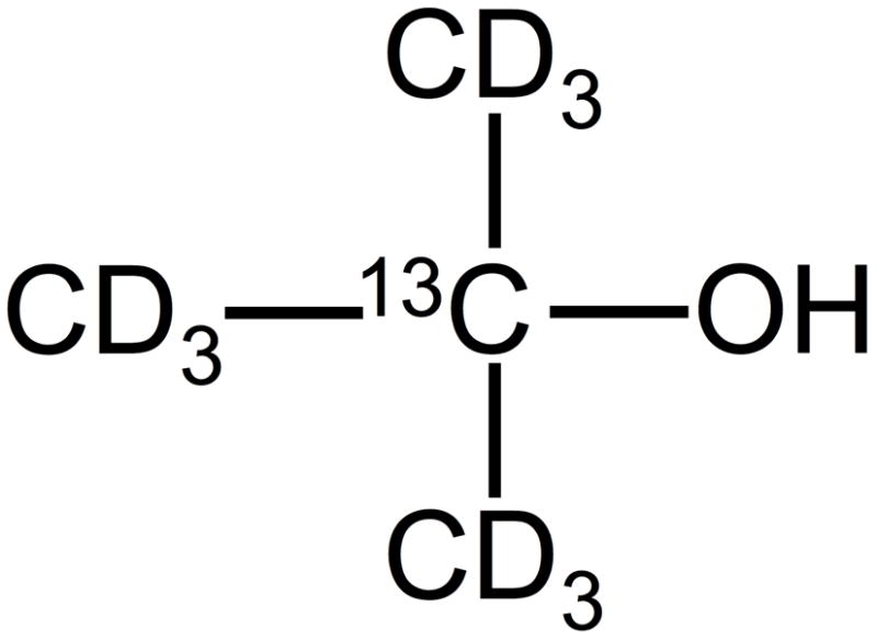
Perdeuterated ¹³C labeled 2-methylpropan-2-ol. In aqueous solution, the OH group is protonated by exchange.

2-methylpropan-2-ol has several features that make it a particularly attractive agent for perfusion imaging. The toxicity of 2-methylpropan-2-ol is low and has been well documented in the literature. These studies have shown that 2-methylpropan-2-ol is metabolized to form the excretory metabolites t-butanol-glucuronide, 2-methyl-1,2-propanediol, and 2-hydroxyisobutyrate. Its half-life in blood is roughly 5–7 hours (20,21). Although the diffusibility of 2-methylpropan-2-ol has not been previously documented in the literature, its octanol-water partition coefficient (log KOW) is 0.35 (22), indicating a comparable affinity for aqueous and lipid environments and suggesting that it should diffuse freely in tissue. Many other alcohols, including ethanol and n-butanol, are known to be freely diffusible in the brain (23,24). In addition, 2-methylpropan-2-ol has long T₁ and T₂ relaxation times when labeled as shown in Fig. 1. Finally, this material can be readily hyperpolarized using dynamic nuclear polarization (DNP) (25–28).

Measurement of 2-methylpropan-2-ol with balanced steady state free precession enables repeated imaging of the bolus passage for an extended period of time. Following a bolus injection, the agent passes slowly through tissue owing to its large distribution volume. The slow bolus passage combined with the long relaxation times of the agent make it possible to image the agent continuously for tens of seconds, thereby enabling extensive signal averaging and robust modeling to extract quantitative estimates of perfusion.

2. Materials and Methods

A. Measurements of 2-methylpropan-2-ol ¹³C relaxation times in blood at 400 MHz field strength

Perdeuterated ¹³C labeled 2-methylpropan-2-ol (Sigma-Aldrich, Saint Louis MO) shown in Fig. 1 was used for all measurements. Initially, the sample was deuterated on all methyl groups as well as the “OD” group. However, when placed in aqueous solution the OD group should be protonated by exchange.

To estimate the in vivo ¹³C relaxation times of 2-methylpropan-2-ol, measurements were performed in a single sample of human blood using non-hyperpolarized 2-methylpropan-2-ol. Blood was drawn into a heparin treated vessel and 20mM sodium citrate was added to prevent coagulation. This procedure was approved by our institutional review board. To prevent separation of blood components, the sample was then sonicated to lyse the red blood cells. Perdeuterated ¹³C labeled 2-methylpropan-2-ol was added to a concentration of 100mM and the mixture was placed in a 5mm NMR tube. The sample was then transferred to a 400 MHz (9.4T) spectrometer (Varian INOVA, Palo Alto, CA) and T₁ was measured using a saturation recovery method. The saturation recovery method was chosen over inversion recovery because it can be performed with a shorter repetition time. The more rapid acquisition of data ensured the stability of the blood sample during the measurements. T₂ was measured using a Carr-Purcell-Meiboom-Gill (CPMG) pulse sequence with an echo spacing of 20ms. A heater was used to maintain the sample at a temperature of 36C throughout the experiment.

B. DNP Hyperpolarization of 2-methylpropan-2-ol

A series of experiments were performed to assess the level of polarization that can be achieved by means of dynamic nuclear polarization (DNP). The DNP process requires that the agent be combined with a paramagnetic radical and frozen in a glassy state at low temperature. Although undiluted alcohols such as n-butanol (IUPAC name butan-1-ol) have been reported to form a glass when frozen rapidly in small drops (29), this approach was not immediately practical for our device. To ensure glass formation, 2-methylpropan-2-ol was therefore combined with glycerol to form a mixture containing 40–50% 2-methylpropan-2-ol by volume.

Preliminary experiments were performed with two radicals: 4-amino-TEMPO (Sigma Aldrich, St. Louis, MO) and “FINLAND” trityl radical (full name tris[8-carboxyl-2,2,6,6-tetramethyl-benzo(1,2-d:4,5-dS)bis(1,3) dithiole-4-yl] methyl sodium salt, GE Healthcare, London UK). The FINLAND radical was found to provide higher levels of solid-state polarization and was employed in all subsequent experiments at a concentration of 15mM.

Three samples containing 50% 2-methylpropan-2-ol by volume mixed with either protonated or deuterated glycerol were prepared. In two experiments, gadolinium contrast (ProHance, Bracco, Italy) was added at a concentration of roughly 1mM. In experiments with pyruvic acid, the addition of gadolinium has been shown to provide higher levels of polarization in the solid state and more rapid polarization buildup at the cost of a shortened ¹³C T₁ in the liquid state (30).

Samples were polarized by means of a commercial DNP hyperpolarizer (Oxford Instruments, Oxfordshire UK) using methods described previously (31). Briefly, material to be polarized was placed in an open sample cup and transferred to the polarizer where it was frozen in liquid helium. The temperature was then lowered to 1.4K and microwaves at a frequency of 94.111 GHz and a power of 50 or 100mW were applied. The microwave power was found to have a negligible impact on the polarization buildup, and was set to 50mW only if the system was unable to maintain a temperature of 1.4K at 100mW. Periodic ‘bake-outs’ were performed as necessary to remove impurities and ensure that the system could maintain a temperature of 1.4K at power levels of at least 50mW. Each sample was polarized until the solid-state ¹³C NMR signal reached at least 95% of the maximum, saturated, level as determined by automated fitting software included with the polarizer. Samples were then flushed from the polarizer using 4ml of water containing 25mg/liter of disodium EDTA and promptly placed within a ¹³C volume coil in a 4.7T horizontal bore animal scanner (Bruker Biospec, Billerica MA). A single FID was then acquired. Several RF pulses were then applied to crush the hyperpolarized magnetization, and the sample was allowed to return to thermal equilibrium over a period of 10 minutes. The thermal equilibrium ¹³C signal from the sample was then measured. The polarization levels were then computed from the ratio of the hyperpolarized signal to the thermal equilibrium signal, as predicted by the Boltzmann distribution.

C. In vivo experiments: animal handling

Two male Wistar rats, weight approximately 210g, were imaged a total of four times separated by at least seven days. All methods were approved by our Institutional Animal Care and Use Committee. Prior to imaging, the rats were anesthetized by inhaled isoflurane at 2–3% concentration. Following induction of anesthesia the level of isoflurane was reduced to approximately 1%. A catheter was placed in the tail vein and connected to a narrow plastic tube approximately 1 meter in length. The animal was placed on an MR compatible bed and anesthesia was maintained using inhaled isoflurane delivered via a nose cone. Throughout the imaging experiment the level of anesthesia was assessed by respiratory monitoring and adjusted as necessary to obtain a respiratory rate of approximately 60 breaths per minute.

Solutions of hyperpolarized 2-methylpropan-2-ol were prepared as described below and administered via the tail vein catheter. The volume administered in the four studies ranged from 1.5 to 3ml as specified in Table 1; in each case the solution was injected at a rate of approximately 100 microliters per second, resulting in bolus durations of 15 to 30s.

Table 1.

Sample compositions for in vivo experiments.

Experiment Number	Glycerol Type	2-methyl-propan-2-ol concentration by volume	Gd Concentration	Quantity Polarized	Dissolution Solvent Volume	Volume Injected(ml)	Polarization Time Constant(minutes)
1	Deuterated	40%	0 mM	242 mg	4 ml	2	64
2	Deuterated	40%	0 mM	214 mg	3 ml	1.5	66
3	Deuterated	50%	1.1 mM	276 mg	4 ml	3	40
4	Protonated	50%	0.9 mM	240 mg	4 ml	3	37

D. Preparation of 2-methylpropan-2-ol for in vivo experiments

All experiments made use of 2-methylpropan-2-ol/glycerol mixtures containing 15mM FINLAND radical as described above. The sample compositions for the four experiments are listed in Table 1. As before, samples were polarized at 50 or 100mW microwave power for sufficient time to achieve a solid-state polarization level of at least 95% of the maximum saturated level. Samples were then dissolved using 3–4ml of 0.45% saline solution containing 250mg/liter of disodium EDTA and transferred to a syringe for injection.

E. Image acquisition

¹³C MR imaging was performed on a 4.7T horizontal bore animal scanner (Bruker Biospin, Billerica MA) using a balanced steady state free precession (bSSFP) sequence. Because hyperpolarized magnetization does not exhibit T₁ recovery, a true steady state is not achieved with this sequence. Instead, the sequence behaves more like a RARE (rapid acquisition with relaxation enhancement) sequence for which a pseudosteady state (32) is achieved until the magnetization gradually decays with T₂ and T₁ relaxation. The use of bSSFP, rather than a conventional RARE sequence, preserves the signal from flowing spins, a property for which bSSFP is well known. Indeed, at the onset of imaging, hyperpolarized spins present in the imaged slice are placed in a pseudosteady state for imaging, while spins that flow into the slice transition to the pseudosteady state as they arrive. The bSSFP method has been advocated previously for hyperpolarized imaging (33), and offers several advantages for perfusion imaging. In particular, when employed with a low tip angle, this sequence can image the hyperpolarized magnetization over an extended period of time that is comparable to the bolus passage time. This aids in quantitation. Moreover, when employed with a short repetition time, the bSSFP RF pulse train serves to refocus the magnetization after each readout, so that the magnetization decays at a rate set by T₂ rather than T₂^*. This prolongs the decay time of the hyperpolarized signal, which can be used to improve the signal-to-noise ratio or to extend the time available for imaging.

The acquisition parameters for each of the four in vivo experiments are summarized in Table 2. Briefly, the bSSFP imaging parameters were TR/TE 4.08ms/2.04ms, 32 kHz Bandwidth, 6–10 cm axial field of view and matrix size 64×64 or 128×128. The slice thickness was 2–3mm. In each experiment, an “alpha/2” preparation pulse was applied and 100 successive images were acquired continuously with a temporal resolution of 248ms (for 64×64 matrix) or 502–521ms (for 128×128 matrix).

Table 2.

Acquisition parameters for in vivo experiments. In last column, ‘after’ means after the completion of the contrast injection, while ‘at beginning’ means at the beginning of the injection.

Experiment Number	Matrix Size	Frame Rate(ms)	Field of View(cm)	Slice Thickness	Approximate Refocusing Tip Angle	Scan Delay Relative to Injection
1	128×128	502	10 cm	3 mm	180	5s after
2	64×64	248	6 cm	3 mm	60	at beginning
3	128×128	521	8.5 cm	2 mm	60	at beginning
4	128×128	521	8.5 cm	2 mm	60	0s after

To assess the timescales for delivery and washout of 2-methylpropan-2-ol, several different scan delays were employed as summarized in Table 2. The scans with short delays enabled monitoring of the arterial signal and inflow of the tracer. Scans that were initiated later allowed full delivery of the bolus into the tissue prior to the application of RF pulses, thereby maximizing the signal available for assessment of the washout of the tracer. In addition, to assess the tolerable dose and concentration of 2-methylpropan-2-ol in the bolus injection, various concentrations were employed across the four experiments.

All images were acquired using a transmit/receive ¹³C surface coil. The coil consisted of two turns of 18-gauge magnet wire and was contoured to match the surface of the head. In order to verify the positioning of the coil and calibrate the ¹³C RF pulses, a vial containing 2.5M ¹³C labeled 2-methylpropan-2-ol in water was placed on top of the coil over the midline of the brain. Prior to administration of hyperpolarized 2-methylpropan-2-ol a series of ¹³C bSSFP scans at varying transmit power were acquired. The image intensity in the vial was used to determine the transmit power that yielded maximum signal, and hence a 180° refocusing pulse in the vial. 180 seconds were allowed between images to assure complete T₁ recovery. Although the surface coil is expected to have an inhomogeneous B1 profile, the coil and vial were situated with respect to the brain such that this technique is expected to yield a satisfactory, if approximate, estimate of the tip angle near the center of the brain (see also Fig. 3 below). Based on this calibration procedure, the refocusing pulse was set to either 60° or 180° as summarized in Table 2.

Fig. 3.

(a). Axial proton image showing rat brain and t-butanol/water vial. Panels (b)–(e) show ¹³C images acquired with 2.08s temporal resolution following administration of hyperpolarized t-butanol. In panel (e), arrows indicate bright signal from venous blood (see text).

Images were reconstructed by zero-filling the raw data to a 512-by-512 matrix size followed by Fourier transformation using MATLAB (The Mathworks, Natick MA). The phase of each complex image was adjusted by applying a constant overall phase correction (for Experiments 1,3 and 4) as well as a phase correction that was linear with position along the read direction (for Experiment 2). The latter phase correction was necessitated by a slight offset of the center of k-space for this particular acquisition. All phase corrections were constant with respect to time. The final images were then obtained by taking the real part of these phased images.

F. Estimation of in vivo relaxation times

Images acquired with the above methods can be used to obtain estimates of the in vivo T₁ and T₂ relaxation times of 2-methylpropan-2-ol. These estimates are at best approximate owing to the use of a transmit/receive surface coil with an inhomogeneous B1 field as well as uncertainties on the ¹³C tip angle. Keeping these caveats in mind, however, the decay rate of the image intensity at a given tip angle can be related to T₁, T₂, and the blood flow in the tissue. The signal decay rate can be converted to estimates of T₁ and T₂ using previously reported measurements of cerebral blood flow in rats under isoflurane anesthesia (34).

In the bSSFP steady state with refocusing tip angle α the magnetization is maintained at an angle α/2 with respect to the main magnetic field and undergoes both transverse and longitudinal decay. In addition, the signal intensity will decay owing to outflow of the tracer. For a freely diffusible tracer with blood/tissue partition coefficient λ in a tissue perfused at flow rate f, the net decay time T is given by

$$\frac{1}{T}=\frac{{cos}^2(\alpha /2)}{T_1}+\frac{{sin}^2(\alpha /2)}{T_2}+\frac{f}{\lambda }.$$ (1)

The first two terms on the right hand side of Eq. (1) describe the signal decay rate in the bSSFP steady state in the absence of flow (35). The last term incorporates the effect of tracer outflow (5). Note that for the short echo spacings employed for the in vivo studies, the effects of microscopic field inhomogeneities are largely refocused and the decay rate depends on T₂ rather than T₂*.

To apply Eq. (1) for estimation of the relaxation times, an estimate of f/λ is required. For rats under isoflurane anesthesia, the whole-brain average of the flow rate is 127±29ml/100g/min (34). The partition coefficient λ is defined as the ratio of the quantities of the tracer in 1ml of blood and 1g of tissue when tissue and blood are in equilibrium. Although the partition coefficient λ of 2-methylpropan-2-ol has not been measured, measurements using the closely related compound n-butanol yield λ = 0.77±0.29 ml/g (36). Based on these values, we obtain f/λ = 0.027±0.012 s⁻¹, where we have combined, in quadrature, the error on λ with an additional 20% error to account for uncertainties in f and differences between n-butanol and 2-methylpropan-2-ol.

The considerations of the preceding paragraph apply only to static magnetization in the imaging plane; magnetization outside the imaging plane undergoes free longitudinal decay with the usual T₁ relaxation time and dilution by fresh inflowing blood. The net decay rate given by substituting α=0 in Eq. (1): 1/T=1/T₁+f/λ. As a result, fresh venous blood flowing into the imaging plane should show high persistent signal relative to static tissue, particularly at high tip angles.

3. Results and Discussion

A. Relaxation times in blood at 400 MHz field strength

In Figure 2 we display saturation recovery measurements of T₁ (left) and CPMG measurements of T₂ (right) in blood. Fits to the data yield T₁=46±4s and T₂=0.55±0.03s. These relaxation times, measured at 9.4T, are not expected to coincide exactly with in vivo measurements at 4.7T. However, they do qualitatively support the expectation that ¹³C 2-methylpropan-2-ol should have relatively long relaxation times in vivo.

Fig. 2.

Measurements of the relaxation times of the quaternary ¹³C of 2-methylpropan-2-ol in blood at 9.4T and body temperature: saturation recovery measurements of T₁ (left) and CPMG measurements of T₂ (right).

B. Polarization of 2-methylpropan-2-ol

The sample compositions and polarization values for the polarization measurements are given in Table 3. The results show that both protonated and deuterated glycerol yield 5–10% polarization levels. Gadolinium does not appear to dramatically shorten the polarization time constant, which ranges from 37 to 43 minutes for the four samples in Table 3, nor does it increase the measured polarization in the liquid state. Polarization measurements in the solid state (not included in Table 3) show that addition of gadolinium can increase the solid-state polarization by a factor of 1.1 or more. However, these gains in polarization appear to be offset by the shortened ¹³C T₁ in the liquid state. The higher polarization level obtained with Sample 1 may be a result of sample composition or, alternatively, may be a consequence of the smaller sample size. We speculate that smaller samples form superior glasses because they freeze more rapidly than larger samples, and that this superior glass formation leads to higher polarization levels. By comparison, typical polarization levels obtained with DNP at 3.35T and 1.2–1.4K include 5% polarization for [5-¹³C]-glutamine (37) and 14–28% for [1-¹³C]-pyruvic acid (38). Although many aspects of 2-methylpropan-2-ol polarization remain to be explored, these data show that polarization levels comparable to those achieved previously can be obtained with relatively straightforward sample preparation techniques.

Table 3.

Sample compositions and polarization measurements.

Sample	Glycerol Type	t-Butanol Concentration by Volume	ProHance Concentration	Quantity Polarized	Polarization Constant(minutes)	Estimated Polarization
1	Protonated	50%	0.9 mM	50 mg	43	10%
2	Deuterated	50%	1.1 mM	231 mg	42	5%
3	Deuterated	50%	0 mM	226 mg	37	6%

C. In vivo images

Images were successfully acquired in all studies. There were no signs of distress, e.g. respiratory rate elevation, during the injection and animals survived repeated studies in apparent good health. Fig. 3 shows images acquired using the parameters from Experiment 1 given in Tables 1 and 2. Fig. 3a shows an axial T₂ weighted proton image of the rat head and a vial, described above, containing 2.5M ¹³C 2-methylpropan-2-ol in water. Figs. 3b–e show a series of ¹³C images acquired after administration of hyperpolarized 2-methylpropan-2-ol. The temporal resolution of the underlying acquisition was 502ms per image; these images have been averaged in groups of four to yield 2.08s temporal resolution. The ¹³C signal strength from the vial seen in Fig. 3a is insufficient to make it readily visible in the ¹³C images shown in Figs. 3b–e. However, in an image obtained by averaging all 100 frames (not shown), the vial is indeed visible.

Figs. 4a–j show ¹³C images acquired in Experiment 3, averaged 10 frames at a time to obtain 5.2s temporal resolution. In this case, the lower refocusing flip angle (60° rather than 180°) results in slower consumption of the hyperpolarized magnetization and a longer time window for image acquisition. Indeed, following the peak signal (presumably corresponding with the first pass of the bolus) occurring in Fig. 4c, the signal persists for tens of seconds afterward. Fig. 4k shows an SNR-optimal perfusion-weighted average of all 100 frames acquired in Experiment 3, described in more detail below.

Fig. 4.

(a)–(j). Frames acquired in Experiment 3, averaged to obtain 5.2s temporal resolution. Panel (k) shows SNR-optimal weighted average of all 100 frames.

These images can be used to quantify the signal-to-noise ratio attainable by these methods, to estimate the in vivo relaxation times of 2-methylpropan-2-ol, and to assess the ability of this agent to diffuse through brain tissue. The following sections address each of these topics.

D. Signal-to-noise ratio

Signal-to-noise ratio (SNR) can be quantified either in terms of the SNR of a single k-space acquisition or in terms of a suitable temporal average of frames. In Fig. 5 we display the first 502ms frame acquired during Experiment 1, expressed in SNR units. The SNR has been computed by dividing the signal in each pixel by the RMS noise in a noise-only region consisting of 100 columns of pixels adjacent to the right-hand edge of the image (this noise-only region has been cropped out in Fig. 5 to show the brain more clearly). In this example, the 2-methylpropan-2-ol bolus has been fully delivered into the brain tissue, and the high flip angle maximizes the available signal. The SNR over the bulk of the brain is in the range of 6–12.

Fig. 5.

The SNR of the first 502ms frame from Experiment 1. The scale is given by the bar at right.

Given the long residence time of 2-methylpropan-2-ol in tissue (see Sections 3E, 3F below), it is unlikely that the 502ms temporal resolution of Fig. 5 would be needed for perfusion quantification. An alternative measure of SNR is provided by an SNR-optimal weighted average of the entire set of 100 images. The optimal SNR is obtained by averaging the frames with a weighting factor proportional to the average signal intensity in the brain. More explicitly, the averaging procedure begins with forming the simple average of all the frames to be included in the final image. A pixel-by-pixel binary mask is then constructed which is equal to 1 in pixels that have SNR greater than 4 and 0 otherwise. The weighted average is then formed by averaging the frames with a weight proportional to the sum of the pixel magnitudes in each frame multiplied by the binary mask. Fig. 6 shows the weighted average images for Experiments 1–4 in SNR units. The peak SNR is on the order of 20–40 in all studies. In Experiments 1 and 4 the imaging sequence was initiated after bolus administration and the late frames show very little signal. Hence in Experiment 1 only the first 20 frames were included in the average, while in Experiment 4 the first 50 frames were included.

Fig. 6.

(a)–(d). SNR-optimal averages of data from Experiments 1 to 4 (a–d, respectively), displayed in SNR units. The bar to the right of each image specifies the SNR scale.

Detailed SNR comparisons between the experiments will depend on a variety of factors including the 2-methylpropan-2-ol dose, the polarization, the slice thickness, the in-plane resolution, and the RF tip angle. In addition, although respiratory monitoring was employed during the studies, variations in other physiological parameters may also influence the results. For purposes of perfusion imaging, the dependence on tip angle is of particular interest, as it impacts the signal persistence time as well as the SNR of each frame. The reduction in refocusing tip angle from α=180° in Experiment 1 to α=60° in Experiments 2–4 might naively be expected to result in a 2-fold reduction in SNR because the transverse magnetization is proportional to sin(α/2). However, this reduction in SNR is partially compensated by the longer persistence time of the signal at lower tip angles, which provides a longer time window for signal averaging. This is apparent from the comparison between Experiment 1 (with 3mm slice and 781 micron in-plane resolution) and Experiment 3 (with 2mm slice and 664 micron in-plane resolution). On the assumption that the two studies were performed under nearly equivalent physiological conditions, the higher resolution and lower tip angle of Experiment 3 would naively result in a substantial (~4-fold) reduction in SNR relative to Experiment 1. However, the images of Fig. 6 show comparable SNR in brain tissue for Experiments 1 and 3. The three bright dots above and on either side of the brain in Experiment 1 are the result of a venous time-of-flight effect described below, and are not directly relevant to this comparison.

The results of Figs. 5 and 6 can be evaluated by comparing with a recent ASL study in the rat brain, which reported SNR values in the range of 4.7–6.7 for perfusion weighted images acquired with 24s total scan time (39). These images were acquired at 2.35T field strength with 4×2 cm field of view, 128×64 matrix size, and 2mm slice thickness. After convolution with a Gaussian kernel, the effective in-plane resolution was approximately 625 microns. Direct comparisons to the results of Figs. 5 and 6 are complicated by differences in field strength (2.35T versus 4.7T) and by the use of a smaller (1 cm) surface coil in the ASL study, which should provide higher local SNR than the 3 cm surface coil employed here. Nevertheless, the SNR values in Figs. 5 and 6 compare favorably to those obtained with relatively mature ASL techniques.

E. Estimation of in vivo relaxation times

The data from Experiment 1, which were acquired after the arrival of the bolus using a high tip angle, can be used to estimate T₁ and T₂. Figs. 7a,b display fits to the signal decay time for representative pixels in the central region of the brain and in venous blood at lower right in Fig. 3. Fig. 7c shows a pixel-by-pixel fit to the decay rate. The fitted decay time constant in regions of static tissue in the brain is in the range 2–4s. At a tip angle of 180°, Eq. (1) together with the above estimate f/λ = 0.027±0.012s⁻¹ (see Sec. 2F) implies T₂~2–4s. The fit also shows that venous signal seen above and on either side of the brain decays with a time constant of 20s. Using Eq. (1) with α=0 as outlined in Sec. 2F yields T₁=(1/T-f/λ)⁻¹=43±24s, a value comparable to that found in blood at 9.4T (see Fig. 2).

Fig. 7.

Fits to the signal decay time T in venous blood (a) and in brain tissue (b). Panel (c) shows pixel-by-pixel map of the decay rate across the field of view. The bar at far right is in units of seconds.

The data of Experiments 2–4 provide a consistency check on the results of the preceding paragraph, demonstrate the extended signal decay times obtained by imaging at a lower flip angle, and illustrate the slow washout of the tracer. These characteristics enable imaging of 2-methylpropan-2-ol over extended periods of time. Fig. 8 shows pixel-by-pixel fits to the decay time after the first pass of the bolus in Experiments 2–4. For the regions of interest highlighted by yellow squares, the decay times are 11±2s, 18±4s, and 19±5s for Experiments 2, 3 and 4 respectively (mean±standard deviation within the ROI). By comparison, for T₁=43±24s, T₂=3±1s, f/λ=0.027±0.012s⁻¹, and α=60°, Eq. (1) predicts a decay time constant T=8–22s, consistent with the measurements of Fig. 8.

Fig. 8.

Pixel-by-pixel fits to the decay time in Experiments 2,3 and 4 (a–c, respectively). The bar at far right is in units of seconds.

F. Evidence for free diffusibility of 2-methylpropan-2-ol in brain tissue

The data of the preceding sections also provide evidence for the free diffusibility of 2-methylpropan-2-ol in the brain. Freely diffusible agents have at least two characteristics that differentiate them from intravascular agents: first, they have a significantly longer residence time in tissue than intravascular or partially permeable agents; and second, the venous signal from a diffusible agent is comparable to the signal from extravascular tissue, whereas the venous signal from an intravascular agent is stronger than the signal in tissue.

More quantitatively, in brain tissue perfused at a flow rate of 127±29ml/100g/min (34) and having a blood volume of 5mL/100g, a purely intravascular agent would be expected to pass through the brain in 2–3s. A freely diffusible agent, however, would have residence time of roughly 50s. The blood volume also implies that an intravascular agent should have a venous signal roughly 20 times larger than the signal in tissue. By contrast, a diffusible agent distributes freely through the extravascular space, resulting in roughly equal concentrations of the agent in the tissue and the veins. Consequently, in the absence of relaxation or time-of-flight effects, the venous signal should be equal to the signal in tissue.

The data displayed in Fig. 8 (particularly those from Experiments 3 and 4) imply a lower bound on the residence time of 2-methylpropan-2-ol in tissue. Indeed, the signal decay in Experiments 3 and 4 is hastened by the application of the bSSFP RF pulse train, and even in the presence of these pulses the signal persistence time is 18–19s. In addition, the persistence of the venous signal shown in Fig. 7a implies a residence time of not less than 20s, as this decay rate includes the effects of both washout and T₁ decay. Taken together, these measurements imply a tissue residence time well in excess of what would be expected for an intravascular or partially permeable agent. However, these data are readily accommodated by the hypothesis that 2-methylpropan-2-ol diffuses freely.

Comparisons of the venous and extravascular signal intensities can be seen in Figs. 4–6. In all cases, the two compartments show comparable signal intensity, providing further support for the free diffusibility of 2-methylpropan-2-ol in brain tissue. The locations of prominent veins seen in Experiment 1 have been noted in Fig. 3, which shows bright venous signal after the first pass of the bolus owing to a time-of-flight effect. In the first frame of Experiment 1 (shown in Fig. 5) the tissue and venous signals are comparable.

4. Conclusions

This initial study has demonstrated that ¹³C hyperpolarization offers an interesting option to improve perfusion imaging studies. Though DNP hyperpolarization has received more attention for metabolic applications, the high image quality and limited technical demands of perfusion imaging with appropriate tracers merits further development.

Apart from the quality of images that can be obtained, the utility of perfusion imaging with hyperpolarized diffusible tracers will depend on the availability and cost of polarizing systems. Polarizer technology is rapidly developing and at this stage, it is difficult to predict future configurations. One potential advantage of the perfusion application, relative to many metabolic studies, is that suitable tracers for Parahydrogen Induced Polarization (PHIP) (40) can be identified. Because PHIP does not require liquid helium temperature or high magnetic fields, it may ultimately be a more economical system for widespread use.

Other important factors for wider use are the toxicity and side effects of the tracer. The 2-methylpropan-2-ol, still mixed with free radical, used in our study is not acutely toxic. However there is limited experience with the side effects and longer-term toxicity of intravenous injection of 2-methylpropan-2-ol. In our study, the dose was primarily limited by the quantity of 2-methylpropan-2-ol that could be polarized using our methods and the dilution of the tracer by glycerol and saline prior to injection. The 2-methylpropan-2-ol dose used here is 500mg/kg, approximately one seventh the LD50 in rats, implying that higher doses may be tolerable. This agent is one of many small molecules with nearly equal solubility in water and lipids that could serve as hyperpolarized perfusion tracers. Identification of the optimal tracers to maximize polarization, T₁ and T₂, and to minimize toxicity is clearly an important next step.

These results highlight the potential of hyperpolarized diffusible tracer perfusion studies. The absence of background intensity, the long residence time in tissue, the relatively slow decay rate and the high potential SNR are major advantages of this approach. Despite the early stage of development, this method provides perfusion weighted images comparable with the best achieved with ASL or dynamic contrast techniques. Improvements in polarization by better glassing methods and lower bath temperatures (41) promise an additional 5 to 10 fold increase in signal for the same dose.

References

- 1.Schlaug G, Benfield A, Baird AE, Siewert B, Lovblad KO, Parker RA, Edelman RR, Warach S. The ischemic penumbra: operationally defined by diffusion and perfusion MRI. Neurology. 1999;53(7):1528–1537. doi: 10.1212/wnl.53.7.1528. [DOI] [PubMed] [Google Scholar]
- 2.Paul AK, Nabi HA. Gated myocardial perfusion SPECT: basic principles, technical aspects, and clinical applications. J Nucl Med Technol. 2004;32(4):179–187. quiz 188–179. [PubMed] [Google Scholar]
- 3.Bruehlmeier M, Roelcke U, Schubiger PA, Ametamey SM. Assessment of hypoxia and perfusion in human brain tumors using PET with 18F-fluoromisonidazole and 15O–H2O. J Nucl Med. 2004;45(11):1851–1859. [PubMed] [Google Scholar]
- 4.Roy PM, Colombet I, Durieux P, Chatellier G, Sors H, Meyer G. Systematic review and meta-analysis of strategies for the diagnosis of suspected pulmonary embolism. Bmj. 2005;331(7511):259. doi: 10.1136/bmj.331.7511.259. [DOI] [PMC free article] [PubMed] [Google Scholar]
- 5.Williams D, Detre J, Leigh J, Koretsky A. Magnetic resonance imaging of perfusion using spin inversion of arterial water. Proceedings of the National Academy of Sciences. 1992;89(1):212–216. doi: 10.1073/pnas.89.1.212. [DOI] [PMC free article] [PubMed] [Google Scholar]
- 6.Herscovitch P, Markham J, Raichle ME. Brain blood flow measured with intravenous H2(15)O. I. Theory and error analysis. J Nucl Med. 1983;24(9):782–789. [PubMed] [Google Scholar]
- 7.Herscovitch P, Raichle ME, Kilbourn MR, Welch MJ. Positron emission tomographic measurement of cerebral blood flow and permeability-surface area product of water using [15O]water and [11C]butanol. J Cereb Blood Flow Metab. 1987;7(5):527–542. doi: 10.1038/jcbfm.1987.102. [DOI] [PubMed] [Google Scholar]
- 8.Neirinckx RD, Canning LR, Piper IM, Nowotnik DP, Pickett RD, Holmes RA, Volkert WA, Forster AM, Weisner PS, Marriott JA, et al. Technetium-99m d,lHM-PAO: a new radiopharmaceutical for SPECT imaging of regional cerebral blood perfusion. J Nucl Med. 1987;28(2):191–202. [PubMed] [Google Scholar]
- 9.Tsuchida T, Yonekura Y, Nishizawa S, Sadato N, Tamaki N, Fujita T, Magata Y, Konishi J. Nonlinearity correction of brain perfusion SPECT based on permeability-surface area product model. J Nucl Med. 1996;37(7):1237–1241. [PubMed] [Google Scholar]
- 10.Brix G, Bahner ML, Hoffmann U, Horvath A, Schreiber W. Regional blood flow, capillary permeability, and compartmental volumes: measurement with dynamic CT--initial experience. Radiology. 1999;210(1):269–276. doi: 10.1148/radiology.210.1.r99ja46269. [DOI] [PubMed] [Google Scholar]
- 11.Gur D, Yonas H, Herbert D, Wolfson SK, Kennedy WH, Drayer BP, Gray J. Xenon enhanced dynamic computed tomography: multilevel cerebral blood flow studies. J Comput Assist Tomogr. 1981;5(3):334–340. doi: 10.1097/00004728-198106000-00003. [DOI] [PubMed] [Google Scholar]
- 12.Johnson DW, Stringer WA, Marks MP, Yonas H, Good WF, Gur D. Stable xenon CT cerebral blood flow imaging: rationale for and role in clinical decision making. Ajnr. 1991;12(2):201–213. [PMC free article] [PubMed] [Google Scholar]
- 13.Seifert H, Blass G, Leetz HK, Voges M. The radiation exposure of the patient from stable-xenon computed tomography. The British journal of radiology. 1995;68(807):301–305. doi: 10.1259/0007-1285-68-807-301. [DOI] [PubMed] [Google Scholar]
- 14.Ostergaard L, Sorensen AG, Kwong KK, Weisskoff RM, Gyldensted C, Rosen BR. High resolution measurement of cerebral blood flow using intravascular tracer bolus passages. Part II: Experimental comparison and preliminary results. Magn Reson Med. 1996;36(5):726–736. doi: 10.1002/mrm.1910360511. [DOI] [PubMed] [Google Scholar]
- 15.Pekar J, Ligeti L, Ruttner Z, Lyon RC, Sinnwell TM, van Gelderen P, Fiat D, Moonen CT, McLaughlin AC. In vivo measurement of cerebral oxygen consumption and blood flow using 17O magnetic resonance imaging. Magn Reson Med. 1991;21(2):313–319. doi: 10.1002/mrm.1910210217. [DOI] [PubMed] [Google Scholar]
- 16.Detre JA, Subramanian VH, Mitchell MD, Smith DS, Kobayashi A, Zaman A, Leigh JS., Jr Measurement of regional cerebral blood flow in cat brain using intracarotid 2H2O and 2H NMR imaging. Magn Reson Med. 1990;14(2):389–395. doi: 10.1002/mrm.1910140223. [DOI] [PubMed] [Google Scholar]
- 17.Petersen ET, Zimine I, Ho YC, Golay X. Non-invasive measurement of perfusion: a critical review of arterial spin labelling techniques. Br J Radiol. 2006;79(944):688–701. doi: 10.1259/bjr/67705974. [DOI] [PubMed] [Google Scholar]
- 18.Johansson E, Mansson S, Wirestam R, Svensson J, Petersson JS, Golman K, Stahlberg F. Cerebral perfusion assessment by bolus tracking using hyperpolarized 13C. Magnetic Resonance in Medicine. 2004;51:464–472. doi: 10.1002/mrm.20013. [DOI] [PubMed] [Google Scholar]
- 19.Johansson E, Olsson LE, Mansson S, Petersson JS, Golman K, Stahlberg F, Wirestam R. Perfusion assessment with bolus differentiation: a technique applicable to hyperpolarized tracers. Magnetic Resonance in Medicine. 2004;52:1043–1051. doi: 10.1002/mrm.20247. [DOI] [PubMed] [Google Scholar]
- 20.Amberg A, Rosner E, Dekant W. Biotransformation and Kinetics of Excretion of Methyl-tert-Butyl Ether in Rats and Humans. Toxicological Sciences. 1999;51:1–8. doi: 10.1093/toxsci/51.1.1. [DOI] [PubMed] [Google Scholar]
- 21.McGregor D. Methyl tertiary-Butyl ether: Studies for Potential Human Health Hazards. Critical Reviews in Toxicology. 2006;36:319–358. doi: 10.1080/10408440600569938. [DOI] [PubMed] [Google Scholar]
- 22.Lide DR. CRC Handbook of Chemistry and Physics. 88. CRC Press; 2008. [Google Scholar]
- 23.Cornford EM, Braun LD, Oldendorf WH, Hill MA. Comparison of Lipid-Mediated Blood-Brain-Barrier Penetrability in Neonates and Adults. American Journal of Physiology. 1982;243(3):C161–C168. doi: 10.1152/ajpcell.1982.243.3.C161. [DOI] [PubMed] [Google Scholar]
- 24.Raichle ME, Eichling JO, Straatmann MG, Welch MJ, Larson KB, Ter-Pogossian MM. Blood-Brain Barrier Permeability of C11-Labeled Alcohols and O15-Labeled Water. American Journal of Physiology. 1976;230(2):543–552. doi: 10.1152/ajplegacy.1976.230.2.543. [DOI] [PubMed] [Google Scholar]
- 25.Overhauser AW. Polarization of Nuclei in Metals. Physical Review. 1953;92(2):411–415. [Google Scholar]
- 26.Carver TR, Slichter CP. Polarization of Nuclear Spins in Metals. Physical Review. 1953;92(1):212–213. [Google Scholar]
- 27.Abragam A, Goldman M. Principles of dynamic nucelar polarization. Reports on Progress in Physics. 1978;41:395. [Google Scholar]
- 28.Ardenkjaer-Larsen JH, Fridlund B, Gram A, Hansson G, Hansson L, Lerche MH, Servin R, Thaning M, Golman K. Increase in signal-to-noise ratio of >10000 times in liquid-state NMR. Proceedings of the National Academy of Sciences of the United States of America. 2003;100(18):10158–10163. doi: 10.1073/pnas.1733835100. [DOI] [PMC free article] [PubMed] [Google Scholar]
- 29.Plueckthun M, Bradtke C, Dutz H, Gehring R, Goertz S, Harmsen J, Kingsberry P, Meyer W, Reicherz G. Polarization measurements of TEMPO-doped butanol targets. Nuclear Instrumentation and Methods in Physics Research Section A. 1997;400(1):133–136. [Google Scholar]
- 30.Ardenkjaer-Larson J, Macholl S, Johannesson H. Dynamic nuclear polarization with trityls at 1.2 K. Appl Magn Reson. 2008;34:509–522. [Google Scholar]
- 31.Kohler SJ, Yen Y, Wolber J, Chen AP, Albers MJ, Bok R, Zhang V, Tropp J, Nelson S, Vigneron DB, Kurhanewicz J, Hurd RE. In Vivo C13 Metabolic Imaging at 3T With Hyperpolarized C13-1-Pyruvate. Magnetic Resonance in Medicine. 2007;58:65–69. doi: 10.1002/mrm.21253. [DOI] [PubMed] [Google Scholar]
- 32.Alsop DC. The sensitivity of low flip angle RARE imaging. Magnetic Resonance in Medicine. 1997;37(2):176–184. doi: 10.1002/mrm.1910370206. [DOI] [PubMed] [Google Scholar]
- 33.Svensson J, Mansson S, Johansson E, Petersson JS, Olsson LE. Hyperpolarized 13C MR angiography using TrueFISP. Magnetic Resonance in Medicine. 2003;50:256–262. doi: 10.1002/mrm.10530. [DOI] [PubMed] [Google Scholar]
- 34.Sicard K, Shen Q, Brevard ME, Sullivan R, Ferris CF, King JA, Duong TQ. Regional cerebral blood flow and BOLD responses in conscious and anesthetized rats under basal and hypercapnic conditions: implications for functional MRI studies. J Cereb Blood Flow Metab. 2003;23(4):472–481. doi: 10.1097/01.WCB.0000054755.93668.20. [DOI] [PMC free article] [PubMed] [Google Scholar]
- 35.Scheffler K. On the transient phase of balanced SSFP sequences. Magn Reson Med. 2003;49(4):781–783. doi: 10.1002/mrm.10421. [DOI] [PubMed] [Google Scholar]
- 36.Herzog H, Seitz RJ, Tellmann L, Rota Kops E, Julicher F, Schlaug G, Kleinschmidt A, Muller-Gartner HW. Quantitation of regional cerebral blood flow with 15O-butanol and positron emission tomography in humans. J Cereb Blood Flow Metab. 1996;16(4):645–649. doi: 10.1097/00004647-199607000-00015. [DOI] [PubMed] [Google Scholar]
- 37.Gallagher FA, Kettunen MI, Day SE, Lerche M, Brindle KM. 13C MR spectroscopy measurements of glutaminase activity in human hepatocellular carcinoma cells using hyperpolarized 13C-labeled glutamine. Magn Reson Med. 2008;60(2):253–257. doi: 10.1002/mrm.21650. [DOI] [PubMed] [Google Scholar]
- 38.Larson PE, Bok R, Kerr AB, Lustig M, Hu S, Chen AP, Nelson SJ, Pauly JM, Kurhanewicz J, Vigneron DB. Investigation of tumor hyperpolarized [1–13C]-pyruvate dynamics using time-resolved multiband RF excitation echo-planar MRSI. Magn Reson Med. 63(3):582–591. doi: 10.1002/mrm.22264. [DOI] [PMC free article] [PubMed] [Google Scholar]
- 39.Wells JA, Lythgoe MF, Gadian DG, Ordidge RJ, Thomas DL. In vivo Hadamard encoded continuous arterial spin labeling (H-CASL) Magn Reson Med. 63(4):1111–1118. doi: 10.1002/mrm.22266. [DOI] [PubMed] [Google Scholar]
- 40.Golman K, Axelsson O, Johannesson H, Mansson S, Olofsson C, Petersson JS. Parahydrogen-Induced Polarization in Imaging: Subsecond 13C Angiography. Magnetic Resonance in Medicine. 2001;46:1–5. doi: 10.1002/mrm.1152. [DOI] [PubMed] [Google Scholar]
- 41.Goertz S, Harmsen J, Heckman C, Hess C, Meyer W, Radtke E, Reicherz G. Highest polarizations in deuterated compounds. Nuclear Instrumentation and Methods in Physics Research Section A. 2004;526(1–2):43–52. [Google Scholar]