

Abstract
Comprehensive proteomic analysis of human plasma or serum has been a major strategy used to identify biomarkers that serve as indicators of disease. However, such in-depth proteomic analyses are challenging due to the complexity and extremely large dynamic range of protein concentrations in plasma. Therefore, reduction in sample complexity through multidimensional pre-fractionation strategies is critical, particularly for the detection of low-abundance proteins that have the potential to be the most specific disease biomarkers. We describe here a 4D protein profiling method that we developed for comprehensive proteomic analyses of both plasma and serum. Our method consists of abundant protein depletion coupled with separation strategies – microscale solution isoelectrofocusing and 1D SDS-PAGE – followed by reversed-phase separation of tryptic peptides prior to LC–MS/MS. Using this profiling strategy, we routinely identify a large number of proteins over nine orders of magnitude, including a substantial number of proteins at the low ng/mL or lower levels from approximately 300 μL of plasma sample.
Keywords: Plasma proteome, Low-abundance protein, Immunoaffinity depletion, Biomarker, MicroSol IEF, SDS-PAGE, LC–MS/MS
1. Introduction
Human plasma (or serum) is one of the most valuable specimens for protein biomarker discovery because it is easily collected and contains thousands of proteins, including those secreted or leaked into the blood by normal cell and tissue processes or cell damage (1). Thus, the presence or change in expression of proteins might potentially indicate the onset and progression of most disease states. However, systematic analysis of the plasma proteome is extremely challenging due to its complexity, the extremely wide dynamic range of protein concentrations that span more than ten orders of magnitude, and the extensive physiological variation among patient samples. The plasma proteome is also dominated by a small number of high-abundance proteins, such as albumin and immunoglobulins, which together constitute more than 80% of the total plasma proteins. In contrast, known disease biomarkers, such as prostate-specific antigen (PSA) and carcinoembryonic antigen (CEA), are low-abundance proteins that are typically found in the low ng/mL to pg/mL range, and most other specific disease biomarkers are likely to be present at similar concentration levels (1–3).
The strategies that have been used most frequently to overcome the dynamic range and sample complexity problems of the plasma proteome are to deplete the major plasma proteins and subject the remaining proteome to multiple fractionation steps for further reduction of sample complexity (4–6). The fractionation steps employed should exploit the orthogonal physicochemical properties of the molecules as a basis for separation. One of the most common multidimensional approaches involves separation of tryptic peptides by strong cation exchange (SCX) followed by reversed-phase (RP) liquid chromatography (7, 8). However, tryptic peptides have limited orthogonal physicochemical properties; therefore, separation methods that involve both proteins and peptides can maximize the effectiveness of fractionation strategies. We have developed several multidimensional protein profiling strategies for a more efficient and comprehensive analysis of the human plasma and serum proteomes. One strategy uses three dimensions of separation coupled with a label-free quantitative comparison of proteomes (9). For an even greater depth of analysis, a 4D method has been developed (5). This strategy utilizes three sequential, and substantially orthogonal, protein pre-fractionation steps followed by online, reversed-phase, tryptic peptide separation prior to mass spectrometry analysis (LC–MS/MS). It is particularly well suited for in-depth cataloging of as many proteins as possible in very complex proteomes, such as human or mouse plasma, rather than for quantitative comparisons of multiple samples. We previously applied this protein profiling method for comprehensive analysis of serum and plasma proteomes and showed that it could detect a large number of proteins from a serum sample in the pilot phase of the Human Proteome Organization Plasma Proteome Project, including 14 of the 20 known proteins in the 1–100 ng/mL range and several proteins in the pg/mL range (5, 10).
2. Materials
2.1. Immunoaffinity Depletion of Major Plasma Proteins from Mouse Plasma or Serum
Mouse plasma or serum (see Note 1).
Milli-Q® water (Millipore, Bedford, MA) or equivalent. “Water” in this text refers to Milli-Q® water unless otherwise specified.
ÄKTA™ Purifier fast protein liquid chromatography (FPLC) system (GE Healthcare, Piscataway, NJ) with 1-mL sample loop.
Multiple Affinity Removal System® (MARS) for mouse serum proteins, 4.6 × 100-mm column (Agilent Technologies, Santa Clara, CA). Store at 2–8°C when not in use.
MARS buffer A. Before use, add the following final concentration of protease inhibitors: 5 mM ethylenediaminetetraacetic acid (EDTA), 0.15 mM phenylmethylsulfonyl fluoride (PMSF), 1 μg/mL leupeptin, and 1 μg/mL pepstatin A.
MARS buffer B. The solution is stable for at least 1 year at 25°C.
50% (v/v) 2-propanol (Optima grade, Fisher Scientific, Pittsburgh, PA).
Stericup® GP Express Plus membrane (Millipore), 0.22-μm filter units, 500 mL capacity.
Amicon® Ultrafree®-MC 0.22-μm microcentrifuge filters (Millipore).
5-kDa MWCO spin separators (Amicon® Ultra 4, Millipore).
10 mM Sodium phosphate buffer, pH 7.4: Prepare 0.1 M stock buffer by dissolving 3.1 g of NaH2PO4 H2O and 10.9 g of anhydrous Na2HPO4 in water to a final volume of 1 L. The stock buffer will have a pH of 7.4 and can be stored for up to 1 month at 4°C. Prepare the working solution by diluting one part with nine parts water.
Beckman J-6B centrifuge with JS-4.2 swinging bucket rotor (Beckman Coulter, Fullerton, CA).
2.2. Microscale Solution Isoelectrofocusing Fractionation
Urea (PlusOne™; GE Healthcare).
3 M Tris–HCl, pH 8.5: Dissolve 36.3 g of Tris in 90 mL water, adjust pH to 8.5 with 1 N HCl, and add water to a final volume of 100 mL.
3 M dithiothreitol (DTT) stock solution: Prepare 10 mL by dissolving 4.63 g in water. Stored in single-use aliquots at −20°C.
N,N-Dimethylacrylamide (DMA) solution (Sigma–Aldrich, St. Louis, MO). The concentration of this reagent is approximately 9.7 M.
Thiourea (Sigma–Aldrich).
3-[(3-Cholamidopropyl)dimethylammonio]-1-propanesulfonic acid (CHAPS) (GE Healthcare).
MicroSol IEF apparatus (ZOOM® IEF Fractionator, Invitrogen, Carlsbad, CA). Reagents for operating the ZOOM® IEF Fractionator were obtained from Invitrogen unless otherwise specified.
ZOOM® focusing buffers, pH 3–7 and pH 7–12.
Electrophoresis power supply (EPS 3501 XL, GE Healthcare) with a capacity of at least 1,000 V that can operate at currents below 1 mA.
pH membranes (ZOOM® disks): 3.0, 4.6, 5.4, 6.2, and 12.0. ZOOM® disks are stable for 3 months when stored at 4°C.
Anode buffer: Prepare 20 mL by mixing 3.5 mL Novex® IEF anode buffer (50×), 9.6 g urea, 3.0 g thiourea, and 7 mL water. Adjust to pH 3.0 with Novex® IEF buffer (50×) and add water to a final volume of 20 mL. Novex® IEF anode buffer (50×) is stored at 25°C and is stable for 1 year.
Cathode buffer: Prepare 20 mL by mixing 2 mL Novex® IEF cathode buffer, pH 9–12 (10×), 9.6 g urea, 3.0 g thiourea, and 7 mL water. Adjust to pH 12.0 with 1 N NaOH, and add water to a final volume of 20 mL. Store Novex® IEF cathode buffer (10×) at 4°C.
MicroSol sample buffer: 8 M urea, 2 M thiourea, 4% (w/v) CHAPS, 1% (w/v) DTT, and 1% (v/v) pH 3–7 and 1% (v/v) pH 7–12 of ZOOM® focusing buffers. Prepare by mixing 4.8 g urea, 1.5 g thiourea, 0.4 g CHAPS, 0.1 g DTT, and 100 μL of each ZOOM® focusing buffers in water to a final volume of 10 mL.
Falcon 3047 24-well, flat-bottom plate (Becton, Dickinson and Company, Franklin Lakes, NJ).
10% NuPAGE® Bis–Tris precast gels (Invitrogen).
Centrifugal filter devices (0.5 mL, 0.22 μm, Millipore).
2.3. 1-D SDSPolyacrylamide Gel Electrophoresis
1 N NaOH, to neutralize acidic samples.
200-Proof ethanol (Sigma–Aldrich), chilled to −20°C.
SDS-solubilizing buffer: 63 mM Tris–HCl, pH 6.8, 0.2 M sucrose, 3% (w/v) SDS, 2 mM Na2EDTA, 1% (v/v) 2-mercaptoethanol, and 1% (v/v) saturated bromophenol blue solution.
XCell SureLock™ Mini-Cell (Invitrogen).
1× NuPAGE® MES running buffer (Invitrogen): Prepare fresh by mixing 50 mL of 20× buffer with 950 mL of Milli-Q®water.
NuPAGE® 12% Bis–Tris, 1-mm thick, ten-well precast gel (Invitrogen). Store at 4°C.
Benchmark protein ladder (Invitrogen).
1-cc Insulin syringe (Becton, Dickinson and Company).
Higgins waterproof India ink (Sanford Corporation, Oak Brook, IL).
Novex® Colloidal Blue Staining kit (Invitrogen).
2.4. High-Throughput In-Gel Trypsin Digestion
Methanol (Optima grade, Fisher Scientific).
Wash solution: 0.1% (v/v) aqueous trifluoroacetic acid, 50% (v/v) aqueous methanol.
PCR cabinet with built-in laminar flow (e.g., Captair®Bio, Erlab) equipped with a light box.
96-Well pierced plates (BioMachines Inc., Carrboro, NC).
V-bottom, 96-well collecting plates (AB-1058, Thermo Fisher Scientific, Waltham, MA). Also used as a trypsin collecting plate and a humidifier plate.
Plate covers for 96-well plates (AB-0751, Thermo Fisher Scientific).
Clean glass plates: 20 × 20 cm and 8 × 12 cm.
Custom-made gel-cutting device consisting of multiple stainless steel razor blades separated by 1-mm Teflon spacer. Alternatively, the MEG-1.5 Gel Cutter (The Gel Company, San Francisco, CA).
Microforcep (Thermo Fisher Scientific).
SpeedVac® Concentrator with 96-well plate centrifuge rotor (Thermo Fisher Scientific).
Eight-channel motorized pipette (Rainin Instrument, Bristol, PA).
37°C Micro-incubator shaker (M-36, Taitec Corporation, Cupertino, CA).
25-mL Reagent reservoirs (Diversified Biotech, Boston, MA) for pipetting with an eight-channel pipette.
Destain solution: 0.2 M ammonium bicarbonate and 50% acetonitrile.
Trypsin solution: 0.02 μg/μL trypsin (Sequencing-grade Modified Trypsin, Promega Corporation, Madison, WI) in 40 mM ammonium bicarbonate, pH 8.0.
Trypsin wash buffer: 40 mM ammonium bicarbonate, 3% formic acid.
Autosampler sample tubes (12 × 32 mm polypropylene vials, Thermo Fisher Scientific).
2.5. Liquid Chromatography–Tandem MS Analysis
Formic acid (LC/MS grade), 10 × 1 mL sealed ampoules (Fluka Analytical, Seelze, Germany).
Hamilton 500-μL glass syringe (GASTIGHT® #1750, Hamilton Company, Reno, NV).
Solvent A: Milli-Q® water with 0.1% formic acid. Add acid using a glass syringe.
Solvent B: Acetonitrile with 0.1% formic acid. Add acid using a glass syringe.
Trap column: NanoACQUITY™ UPLC Symmetry 5-μm C18 trap, 180 mm i.d. × 2 cm long (Waters Corporation, Milford, MA).
Analytical column: NanoACQUITY™ UPLC BEH 1.7-μ C18 column, 75 μm i.d. × 25 cm long (Waters); or self-packed, 25-cm long PicoFrit® column (75 μm i.d./15 μm tip i.d., New Objective, Woburn, MA) with 3-μm 100 Å Magic C18AQ™ resin (Michrom Bioresources, Auburn, CA).
High-performance or ultra-performance LC (UPLC) system, capable of nanoliter flow rates, with a chilled autosampler (e.g., NanoACQUITY™ UPLC, Waters).
Mass spectrometer with fast scan rate (e.g., LTQ Orbitrap XL™, Thermo Fisher Scientific).
MS/MS data analysis software (e.g., Sequest or Mascot).
3. Methods
The protein profiling strategy described here consists of three sequential protein separation steps, i.e., major protein depletion, microscale solution isoelectrofocusing (MicroSol IEF), and 1D SDS-polyacrylamide gel electrophoresis (SDS-PAGE), followed by online, reversed-phase, LC peptide separation prior to mass spectrometry (MS) analysis. Each of these separation steps is designed to reduce the complexity of the plasma proteome incrementally and thus allow a higher amount of sample to be processed or analyzed in subsequent steps. Maximizing the protein load at each separation step is critical to obtain comprehensive, in-depth proteome coverage.
While this multidimensional protein profiling method enables in-depth proteome analysis, it also will increase the total number of samples (and analysis time) for downstream analysis. Therefore, a major consideration before beginning the protocol is to determine the total number of fractions per sample for LC–MS/MS analysis that is desired. In this protocol, the sample number is affected mainly by the number of MicroSol IEF fractions and the separation distance/number of slices per lane for the 1D SDS gels. Increasing the number of fractions will increase the resolution and usually result in the identification of higher numbers of proteins and peptides (depth of coverage) at the expense of longer analysis time per proteome. The method presented here is aimed at maximizing the depth of coverage while keeping the sample size as low as possible.
3.1. Immunoaffinity Removal of Major Plasma Proteins
The first protein fractionation step is the depletion of major plasma proteins. We have examined a number of commercially available dye-based and immunoaffinity methodologies for depleting abundant proteins from human plasma. We found that the immunodepletion methods are more efficient at depleting targeted proteins, typically with greater than 98% removal of most targets and with minimal removal of untargeted minor proteins (11). Since major plasma proteins prevent the identification of lower-abundance proteins, immunoaffinity columns capable of efficiently depleting the most number of major plasma proteins would facilitate the greatest in-depth analysis of the plasma proteome. Aside from human plasma, immunodepletion methods are also available for a few other species, especially mouse and rat, due to their widespread use as animal models for human diseases, toxicology, and drug testing, as well as in protein biomarker discovery. The protocols for immunodepletion of major human and mouse proteins are very similar, although vendor-specific buffers for binding and elution of proteins are usually required. We have previously published protocols for immunodepletion of human plasma using the Sigma ProteoPrep 20®, which removes 20 major plasma proteins (12). In this protocol, we describe the use of the Agilent MARS-Mouse 3® column for depletion of three major proteins from mouse plasma as an example of major protein depletion. The depletion step is important for comprehensive analysis of the plasma proteome because these major proteins constitute approximately 80% of plasma proteins (1, 2). Hence, after depletion, far greater volumes of plasma can be separated by downstream analytical methods:
Transfer the MARS column to room temperature and prepare fresh daily the appropriate amount of Buffer A (see Note 2) and Buffer B. The final volumes needed for each depletion is approximately 50 mL of Buffer A and 25 mL of Buffer B. Filter the buffers through a 0.22-μm filter unit and degas for 5 min at 25°C using vacuum filtration with stirring.
Flush the FPLC system, including the column inlet line, with Buffer A for 15 min at 1 mL/min. Reduce the flow to 0.5 mL/min, remove the top plug of the column, and connect the inlet line to the top of the column, taking care not to introduce air into the column. Remove the bottom plug of the column and connect the detector inlet solvent line. Continue to equilibrate with Buffer A for 5 min at 1 mL/min.
Prior to injection of the first sample of the day, run a blank to remove any residual protein from previous depletions and re-equilibrate the column using Buffer A.
Dilute the required volume of mouse plasma five times with Buffer A. Filter the diluted plasma with pre-rinsed, 0.22-μm microcentrifuge filters to remove particulates. Keep the filtered sample on ice until ready for use (see Note 3).
After the column has fully equilibrated, inject 375–500 μL of diluted plasma at 0.5 mL/min.
Elute the unbound proteins (depleted plasma) from the column with Buffer A at 0.5 mL/min for 10 min. Collect the flow-through fractions and pool the unbound fractions containing protein as it is eluted from the column. Keep the pooled sample on ice.
Elute the bound proteins with Buffer B at 1 mL/min for 14 min. Collect and pool the bound proteins and store on ice (see Note 4). Re-equilibrate the column with Buffer A for 22 min at 1 mL/min.
Repeat steps 5–7 until all samples are processed.
Disconnect and store the column at 4°C in Buffer A.
Replace Buffers A and B with Milli-Q® water and flush the FPLC system, including the detector, for 30 min at 1 mL/min, followed by 50% 2-propanol for 30 min at 1 mL/min.
Pre-rinse two or more 5-kDa MWCO spin separators by centrifuging 2 mL of Milli-Q® water through them, using the J6-B centrifuge at 1,500 × g and 4°C for 10 min.
Pool all unbound fractions and concentrate to 200 μL using the pre-rinsed spin separator.
Desalt the concentrated unbound fraction by adding 1.8 mL of 10 mM sodium phosphate buffer, pH 7.4, and again concentrating to 200 μL. Repeat at least four times to reduce ionic strength and replace the MARS Buffer A.
Rinse the concentrator unit with 50 μL of 10 mM Sodium phosphate, pH 7.4, and combine with the concentrated unbound fraction (see Note 5).
Run proportional amounts of unbound and bound fractions on a SDS-polyacrylamide gel to evaluate the efficiency of protein depletion. Examples of the results produced for mouse plasma, as described in this protocol, as well as for human plasma using the ProteoPrep® 20 column, are shown in Fig. 1.
Fig. 1.
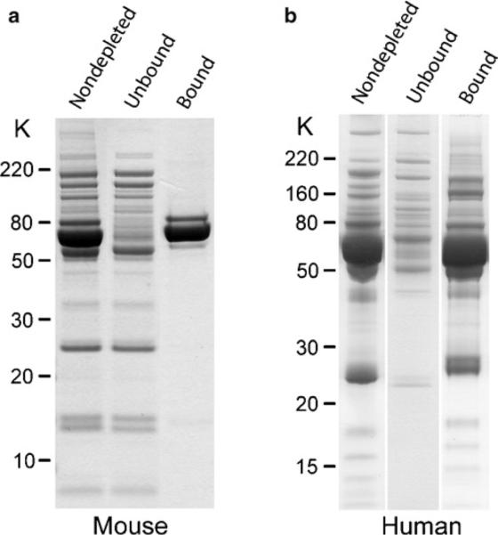
Comparison of major protein depletion from mouse and human plasma. (a) Depletion of three major mouse proteins (albumin, IgG, and transferrin) using the Agilent MARS Mouse 3 LC-Column®. (b) Depletion of 20 major human proteins using Sigma ProteoPrep® 20 FPLC system. In both cases, depletion of major proteins enhanced detection of lower-abundant plasma proteins. Samples were separated on a NuPAGE® Bis–Tris gel and stained with colloidal Coomassie® blue.
3.2. MicroSol IEF Fractionation of Unbound Proteins
Solution IEF is used as the second fractionation step to further reduce the complexity of the plasma proteome. Solution IEF separation devices that rely on immobiline-buffered membranes for protein separation are capable of very high-resolution separations because membrane partitions can be selectively made at precise pH values, and proteins with pI values differing by as little as 0.01 pH units can be separated (13, 14). We developed a convenient, multi-chamber solution IEF device that was subsequently commercialized as Invitrogen's ZOOM® IEF Fractionator (14–17).
Solution IEF is performed using the ZOOM® IEF Fractionator, which contains seven 700-μL separation chambers and can, therefore, provide a maximum of seven pI fractions when eight immobiline/acrylamide partition disks are used. There is, however, great flexibility in its assembly, offering different configurations of immobiline/acrylamide partition disks and numbers of fractions for analyzing diverse types of samples and for different research needs (14, 17). This protocol describes a four-separation chamber configuration that we routinely use for comprehensive plasma proteome analysis:
Add sufficient 3 M Tris–HCl, pH 8.5, and dry urea to 3 mg of depleted plasma to yield final concentrations of 8 M urea, 20 mM Tris–HCl, pH 8.5, in a 500-μL final volume (see Note 6).
Add 3 M DTT to a final concentration of 20 mM to reduce disulfide bonds. Mix, blanket with argon, and incubate at 25°C for 30 min with gentle agitation.
Add DMA to a final concentration of 50 mM to alkylate cysteine residues. Mix, blanket with argon, and incubate at 25°C for 30 min with gentle agitation (see Note 7).
Terminate the reaction by adding DTT to a final concentration of 64.8 mM (1% DTT), taking into account that it already contains 20 mM DTT. Mix well. Incubate at 25°C for 15 min (see Note 8).
Add dry urea, thiourea, CHAPS, and ZOOM® focusing buffers, pH 3–7 and 7–12, to a final concentration of 8 M urea, 2 M thiourea, 4% (w/v) CHAPS, and 1% (v/v) each of ZOOM focusing buffers, pH 3–7 and 7–12 (the same final concentration as in the MicroSol sample buffer). If necessary, re-adjust DTT to 64.8 mM final concentration. The final sample volume should be less than 2,680 μL (step 8). Mix well.
Clean and assemble the ZOOM® IEF Fractionator according to the manufacturer's instructions. Assemble a four-chamber separation device with adjacent chambers separated by membrane disks in the following order: pH 3.0, 4.6, 5.4, 6.2, and 12.0 (see Note 9). The first two and the last chambers are blank chambers without a disk separating them from the anode and cathode chambers.
Load approximately 17.5 mL anode buffer (pH 3.0) and cathode buffer (pH 12.0) into each electrode reservoir of the chamber. Note that chambers 1, 2, and 7 will also contain the anode or cathode electrode buffer when the four-separation-chamber configuration is used.
Dilute the sample to a final volume of 2,680 μL (670 μL for each of the four chambers) with MicroSol sample buffer. Remove any undissolved particulate material by centrifugation at 16,000 × g for 10 min at 25°C. Load 670 μL of the diluted sample in all four chambers, taking care not to introduce bubbles into the chambers (see Note 10).
Insert sample chamber port plugs into all sample chambers. Place the lid on the assembled fractionator and focus the sample by applying an electrical field. Set the maximum limits of the power supply to 750 V, 1 mA, and 1 W. The separation is initially limited by current, and as the conductivity falls, the voltage rises until 750 V is achieved. Continue the separation until a stable low current is reached (see Note 11).
After focusing is completed and prior to disassembling the device, remove the fractionated samples in chambers 3–6 through the fill ports using a gel-loading pipette (see Note 12). Transfer the contents into individual microfuge tubes. Rinse each chamber with 100 μL MicroSol sample buffer and combine with the corresponding fractions.
Disassemble the device. Place each of the membrane disks into individual wells of a 24-well flat-bottom plate, each containing 100 μL of MicroSol sample buffer.
Incubate at 25°C with shaking for 30 min.
Transfer the membrane disk extracts to individual microfuge tubes. Add another 100 μL of MicroSol sample buffer to the wells containing the membrane disks. Repeat step 12. Combine the second membrane disk extract with the first extract (see Note 13).
Run each fraction and membrane disk extract on a SDS polyacrylamide gel to evaluate the ZOOM® IEF separation. An example of the results produced is shown in Fig. 2.
Fig. 2.
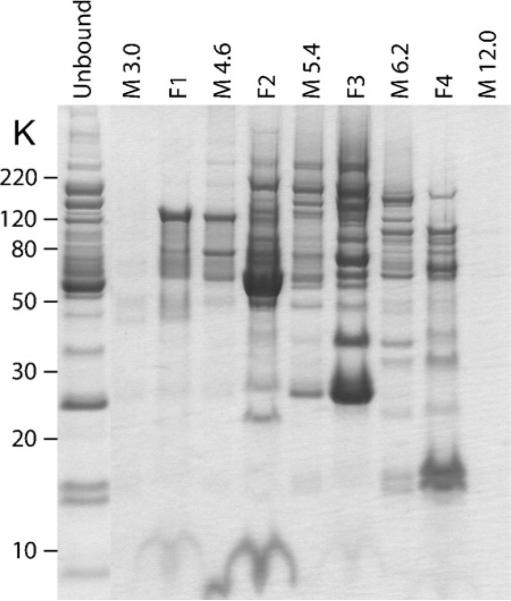
MicroSol IEF fractionation of a depleted mouse plasma sample. Depleted plasma proteins (unbound) were separated by MicroSol IEF using a four-chamber configuration. The membrane extracts (M) and the pH values are indicated. The four MicroSol IEF fractions are indicated by F1–F4. Samples were run on a 10% NuPAGE® Bis–Tris gel with MES buffer and stained with colloidal blue. A good separation is evident from the presence of unique protein bands in each of the MicroSol IEF fractions.
3.3. Separation of MicroSol IEF Fractions by 1D SDS-PAGE
The third fractionation step utilizes 1D SDS-PAGE to separate proteins in each MicroSol IEF fraction and membrane disk extract efficiently according to their molecular weights. SDS-PAGE not only offers reproducible separation, but also provides a convenient method for sample clean-up prior to trypsin digestion. This protocol uses commercial precast gels for convenient and reliable protein separation. An important parameter to consider for SDS-PAGE is the length of electrophoretic separation, as it will affect the number of samples for downstream MS analysis and gel volume per trypsin digest. Generally, complex samples are electrophoresed for a longer distance to obtain better resolution, and less complex samples can be run for a short distance without drastically affecting the depth of analysis. In all cases, a maximum amount of proteins that will not cause excessive band distortion should be loaded in each gel lane to facilitate in-depth protein identification:
Precipitate desired amounts of each MicroSol IEF fraction and membrane disk extract with ethanol. Neutralize the F1 (pH 3.0–4.6) fraction to pH 7 with 1 N NaOH prior to ethanol precipitation. Add nine volumes of 200-proof ethanol (−20°C) to the samples.
Incubate the samples overnight on ice at 4°C. Centrifuge the samples for 30 min at 4°C. Carefully remove the supernatant without disturbing the pellets, and air-dry pellets briefly in a fume hood. Dissolve the pellets with the appropriate volume of SDS-solubilizing buffer (see Note 14).
Use separate precast gels for each fraction. Measure a distance of 1 or 3 cm from the bottom of the wells and mark the position on the gel cassette with a permanent marker. Use the 1-cm-marked gels for membrane disk extracts and the 3-cm-marked gels for F1–F4 samples (see Note 15).
Clean the gel unit and assemble as per the manufacturer's instructions. Fill the gel tank with 1× MES running buffer (see Note 16).
Heat the samples and protein standard at 90°C for 2 min. Load at least three lanes for each sample.
Run gels at 200 V constant. Terminate the electrophoresis when the bromophenol blue dye front reaches the 1- or 3-cm line.
Remove the gel from the unit chamber. Discard one of the plastic plates to expose the gel. Mark the dye front with a small amount of black India ink using a 1-cc syringe needle.
Fix and stain all gels using Colloidal blue stain according to the manufacturer's instructions. Store destained gels in clean Ziploc® plastic bags at 4°C until ready for trypsin digestion. Representative results are shown in Fig. 3.
Fig. 3.

Composite gels showing optimized loading of MicroSol IEF samples of fractionated mouse plasma for in-gel trypsin digestion. Samples were concentrated by ethanol precipitation and maximal amount of sample (not producing visible streaks) was loaded on a 12% NuPAGE® Bis–Tris gel. Each MicroSol IEF fraction and membrane extract were separately electrophoresed for 3 and 1 cm from the bottom of the sample well, respectively. All gels were stained with colloidal Coomassie® blue.
3.4. In-Gel Trypsin Digestion of Proteins
Due to the large number of digests that need to be performed, we have developed a high-throughput protocol that utilizes a 96-well plate format for in-gel digestion. Reagents are rapidly dispensed using an eight-channel pipette from disposable reservoirs, and gel slices are processed in 96-well plates with pierced bottoms that allow rapid centrifugal removal of reagents. This protocol allows a single person to perform up to 384 tryptic in-gel digests (4 × 96-well plates) easily in parallel:
Perform all procedures in a PCR hood to minimize airborne contamination. Clean all 96-well plates and glass plates by washing with 50% methanol containing 0.1% trifluoroacetic acid, followed by rinsing with methanol. Air-dry in the PCR hood.
Stack a 96-well pierced plate on top of a V-bottomed 96-well collecting plate.
Place the gel on a clean 20 × 20-cm glass plate. Cover the gel with just enough Milli-Q® water to prevent dehydration during the slicing process. Cut the gel lane using the gel cutting device into 1 × 4 mm slices (see Note 17). Transfer the gel slices into separate wells on the 96-well pierced plate using a microforcep. Combine gel slices from three adjacent replicate lanes (same molecular weight range) into the same well on the pierced plate (see Note 18).
Add 100 μL of destain solution to each gel-containing well using an eight-channel pipette. Place a cover on top of the pierced plate and incubate at 37°C for 30 min with shaking.
Remove destain solution from the pierced plate into the collecting plate by spinning for 1 min in the SpeedVac® concentrator. Discard destain solution from the collecting plate and put it back under the pierced plate.
Dry the gel slices under vacuum in a SpeedVac® at 37°C for approximately 30 min. Replace the collecting plate with a clean 96-well plate (trypsin collecting plate) for trypsin digestion.
Add 40 μL of trypsin solution to each gel-containing well (see Note 19). Place an 8 × 12-cm glass plate on top of the pierced plate to prevent sample loss by evaporation. To further prevent evaporation of samples, add 80 μL of water to the wells of another 96-well collecting plate (humidifier plate) and place it under the trypsin collecting plate. Assemble the three plates, together with the glass plate and cover, in a Ziploc® bag to create a humidified chamber. Incubate the plate for 16 h at 37°C with no shaking.
Collect trypsin digests into the trypsin collecting plate with 1-min spin in the SpeedVac® concentrator. Add 30 μL trypsin wash buffer to each gel-containing well in the pierced plate and incubate with no shaking at 37°C for 30 min (see Note 20). Combine this tryptic supernatant with the first tryptic supernatant on the trypsin collecting plate with 1-min spin in the SpeedVac® concentrator.
Transfer the samples into cleaned autosampler vial and load directly into the LC–MS/MS system, or freeze the samples at −20°C until needed.
3.5. Reversed-Phase Separation of Tryptic Peptides and Tandem MS Analysis
Tremendous progress has been made in the field of protein/peptide MS in the past two decades, resulting in a wide variety of commercial mass spectrometers with different types of ionization methods and mass analyzers. Linear ion trap instruments (e.g., Thermo Fisher's LTQ series of instruments) – which feature high-duty cycle, tandem MS (MS/MS) capability, fast scan rates, and high sensitivity – are best suited for comprehensive, in-depth proteomic studies of complex samples (18, 19). Recently, hybrid mass spectrometers have been built that combine the advantages of multiple mass analyzers. One such instrument is the LTQ Orbitrap, which combines the speed and sensitivity of the LTQ with the high resolution and mass accuracy of the Orbitrap mass analyzer (20, 21).
Despite progress in MS instrumentation, successful MS analysis of complex samples requires front-end separations to simplify the extremely complex peptide mixtures prior to MS analysis. This is especially critical for the detection of low-abundance peptides that would otherwise be obscured by higher-abundance signals. The most common front-end separation technique, which is also used here as the fourth separation mode, is reversed-phase, high-performance liquid chromatography (RP-HPLC). Peptides are continuously separated based on their hydrophobicity by RP-HPLC, and the effluent is directly analyzed using tandem MS analysis (LC–MS/MS). The introduction of UPLC systems has enabled the use of longer reversed-phase columns packed with small particle size (<2 μm) resins that result in improved resolution, peak capacity, and sensitivity of peptide separation (8, 22):
Tune and calibrate the LTQ Orbitrap according to the manufacturer's instructions (see Note 21).
Set the autosampler to pick up 4–8 μL of sample (see Note 22). Inject onto the trap column at 5 μL/min for 4 min with 100% Solvent A.
Set the binary solvent manager (UPLC pump) to deliver the following acetonitrile gradient at 0.2 μL/min for peptide separations: 3–28% B over 42 min, 28–50% B over 26 min, 50–80% B over 5 min, 80% B for 4 min, 3% B over 1 min, and hold for an additional 10 min (see Note 23).
To minimize carry-over between samples, run a quick blank gradient at 0.4 μL/min with the following gradient: 3–80% B over 11 min, hold at 80% B for 5 min, back to 3% B in 0.5 min, and hold for an additional 13.5 min.
Set the mass spectrometer to acquire MS/MS in data-dependent mode. Perform full MS scan (m/z 400–2,000) in the Orbitrap with 60,000 resolution at 400 m/z. Trigger MS/MS in the linear ion trap on the six most intense ions exceeding a minimum threshold of 1,000 (see Note 24).
Start flow at 0.5 μL/min with 3% Solvent B through the trap and analytical column for 15 min. Ensure that there is no leakage or blockage by monitoring the system pressure.
Place the sample vials on the chilled 48-well tray in the sample manager (autosampler) and start the MS run (see Note 25). An example of a typical LC–MS/MS run is shown in Fig. 4.
Analyze MS/MS results using software packages such as Sequest (23) or Mascot (Matrix Science, Boston, MA), and combine the results for all LC–MS/MS runs for the proteome using programs such as DTASelect (24) and Scaffold (Proteome Software, Portland, OR).
Fig. 4.

Increased protein/peptide identification with longer LC–MS/MS analysis. Tryptic digests from two different gel slices of a depleted plasma proteome were combined and analyzed by LC–MS/MS. The MS method is identical for both analyses, but two different LC run times (88 and 240 min) were used. Base peak chromatograms indicate that the 88-min run (top) had higher ion intensities (Int) than the 240-min run (bottom), as expected. The 240-min run identified substantially more unique proteins and peptides than the 88-min run, but at the expense of decreased sample throughput. MS/MS spectra were searched using Sequest (23) and then processed using DTASelect (24) and custom software to obtain a comprehensive catalog of the plasma proteome.
Acknowledgments
This work was supported in part by National Institutes of Health Grants CA120393 and CA131582, and institutional grants to the Wistar Institute including an NCI Cancer Core Grant (CA10815) and the Commonwealth Universal Research Enhancement Program, Pennsylvania Department of Health.
Footnotes
Blood samples should be collected in a consistent manner with a well-defined protocol in order to avoid introducing bias related to sample collection and handling. Samples should be stored in aliquots, preferably in liquid nitrogen or at −80°C, to prevent proteolysis or modifications. A recent study suggests that platelet-depleted plasma may be better than serum, which contains a large number of peptides that are thought to be generated as the result of platelets releasing peptides or from its blood-clotting process (25).
Buffer A is prepared fresh with the addition of protease inhibitors to minimize protein degradation.
The column can deplete approximately 75–100 μL of mouse plasma, depending upon the concentration of the samples and the actual column capacity. Typically, we obtained about 1 mg of unbound proteins from 100 μL of mouse plasma. For comprehensive plasma proteome analysis using this 4D method, we generally performed sufficient depletions to have at least 3 mg of unbound proteins for the next fractionation step. Protein concentrations can be determined using the BCA protein assay.
The bound fractions containing the major plasma proteins are usually not analyzed but are frozen for potential future analysis. Prior to storage, neutralize the bound fraction by adding 1 N NaOH to pH 7.0.
Set aside 1–3 mg of unbound fraction for subsequent analysis. Store the remainder in aliquots at −80°C.
The maximum amount of sample that can be separated effectively by MicroSol IEF varies slightly depending upon sample type, loading position, and the number of sample chambers used (14, 17). For most studies, a sample load capacity in the 1–3 mg range is recommended and should be adequate for downstream analysis. Vortex gently to ensure complete protein solubilization and denaturation. This will facilitate reduction and alkylation of all disulfide bonds, which are critical for efficient and reproducible separation of proteins by solution IEF. Since urea is used for sample denaturation, avoid excessive heating of samples to minimize unwanted protein carbamylation.
Do not use iodoacetamide for alkylation, as it will result in high current and interfere with MicroSol IEF separation.
This step not only quenches the alkylation reaction but also ensures that the sample contains a high concentration of DTT to keep any residual unmodified cysteines reduced during subsequent ZOOM® IEF fractionation.
The number of chambers used should be determined based on experimental needs. A seven-chamber approach, especially using custom pH disks (14), will increase the resolution of the separation but will substantially increase the total separation time. A frequent alternative for higher-resolution separation is using a five-chamber separation mode by inserting an additional chamber with a pH 7.0 disk between the pH 6.2 and pH 12.0 disks. Increase the maximum voltage to 1,000 V for five-chamber separations.
In general, a sample is loaded into all separation chambers to allow dilution to the largest possible volume. However, with some samples (e.g., non-depleted plasma), restricting the loading to the middle chamber might result in better focusing. This presumably is because some proteins that are unstable at pH extremes may precipitate before they have sufficient time to move out of the highest and lowest pH chambers. Also, some proteins loaded into the most basic and acidic sample chambers must migrate the longest distance to reach the appropriate chamber at equilibrium.
The separation should be terminated as soon as a stable low current (usually around 0.3 mA) is achieved, because excessive focusing times can result in poorer separation. The total focusing time for 3 mg of plasma sample is approximately 3 h using the conditions described here. Samples containing higher protein loads, high salt concentrations, or higher ampholyte concentrations will usually require much longer separation times, and in some cases, it may not be feasible to reach 750 V or a minimum current below 1 mA.
After the MicroSol IEF run, the volumes in sample chambers may be reduced slightly due to electro-osmosis. Reduction of any fraction to less than 50% of its original volume indicates that the chamber was poorly sealed and the quality of the entire separation will probably be compromised.
Proteins with pI values equal to the membrane pH value will be trapped in the membrane disks and need to be extracted for optimal proteome coverage. Because the membrane disks are in contact with two chambers, the membrane extracts will also contain some proteins from the adjacent chambers (Fig. 2). In this protocol, all membrane extracts are analyzed individually, albeit at a lower gel resolution. Alternatively, the membrane extracts could be combined with an adjacent solution fraction to reduce the number of fractions for downstream analysis. In this case, the membrane disk extracts should be combined to an adjacent solution fraction that displays the protein profile most similar to that determined from the SDS-PAGE analysis.
Concentrate enough of each MicroSol IEF fraction for at least three lanes using a maximum load. We typically combine gel slices of the same molecular weight range from three adjacent replicate lanes to generate larger amounts of the tryptic digest. Generally, fractions with less protein (F1 and F4) can be concentrated up to 20-fold or more, and fractions with more proteins (F2 and F3) can be concentrated up to approximately tenfold. It is recommended to determine the maximum sample load by running an aliquot of the concentrated samples on a SDS-gel prior to running the preparative multiple lane gel.
Using a separate gel for each fraction will avoid contamination from other fractions, especially when maximum volumes are loaded and slight well overflow may occur. Since the sample complexity of membrane extracts is low, running the gel for 1 cm will compress all the protein bands, reducing the size of sparsely populated regions in the gel, and, therefore, reducing gel volumes (improved peptide recovery) and/or fractions for MS analysis (increases throughput). Running the more complex MicroSol IEF fractions for 3 cm typically yields adequate depth of analysis and is a good compromise between increased gel resolution and decreased throughput of MS analysis.
One of the major environmental contaminants identified by MS analysis is keratin. Make sure that the gel units are clean and protect them from dust. Wear gloves and wash gloves with Milli-Q® water before handling the gels.
Using 1-mm slices, a 1- and 3-cm gel lane will result in 10 and 30 gel slices, respectively.
Multiple replicate lanes from each MicroSol IEF fraction are cut and adjacent gel slices are combined to generate a larger amount of tryptic digest for potential additional LC–MS/MS runs. Corresponding gel slices from up to three or four replicate lanes can be digested per well. We prefer to use the custom gel-cutting tool because the width of the razor blade array allows up to four gel lanes to be cut simultaneously, thereby minimizing lane-to-lane variations in the locations of the gel slices. In addition, the sharp razor blades cut into the gel easily without crushing it.
The volume of trypsin solution used is dependent upon the number of gel slices. Use 40 μL for three gel slices. Increase the volume to 50 μL for digesting four gel slices, and reduce the volume to 20 μL for digesting one or two gel slices.
Add 30 μL of trypsin wash buffer for three gel slices. Increase volume to 40 μL for digesting four gel slices, and reduce volume to 15 μL for digesting one or two gel slices.
The major benefit of the Orbitrap mass analyzer is the ability to measure peptide masses accurately with less than 5 ppm error. High mass accuracy greatly increases the confidence of peptide identifications. To maintain this level of accuracy, the mass spectrometer usually needs to be calibrated every 2–3 days. The LTQ Orbitrap can also be run with “Lock Mass” on, which allows for real-time recalibration using polydimethylcyclosiloxane ions present in ambient air (26). However, it is recommended that the Orbitrap mass calibration still be performed regularly even if “Lock Mass” is used during data acquisition.
The injection volume depends upon the amount of protein in the gel slices that were digested. We typically inject 4 μL of digests from slices with very heavy protein loads, and 8 μL for all other gel slices. Generally, nano-C18 columns have a loading capacity of approximately 1–2 μg of tryptic peptides. If protein/peptide quantitation is critical, it is best to use a slightly lower load (~0.5 μg) to ensure that the signals are within the linear range of quantitation.
We find that this 88-min HPLC method is generally sufficient to handle the peptide complexity generated from this protocol. For highly complex peptide samples (e.g., a combination of multiple gel digests or non-MicroSol IEF fractionated samples), a longer gradient will certainly result in greater depth of peptide identifications. An example is shown in Fig. 4.
Other LTQ Orbitrap parameters that we typically use are as follows. Preview mode for FTMS master scans is enabled to allow parallel collection of MS/MS data in the linear ion trap, while the Orbitrap analyzes the full MS scan. Ions are isolated for MS/MS using an isolation width of 2.5 Da. Dynamic exclusion is enabled to prevent repeated analysis of the same ion (m/z within 5 ppm) with a duration of 45 s. The monoisotopic precursor selection is enabled to ensure correct reporting of the peptide monoisotopic mass, and charge state screen is used to exclude singly charged ions (mainly caused by chemical noise) from MS/MS analysis.
Always run a reference digest prior to running actual samples to ensure that the LC–MS/MS system is operating optimally.
References
- 1.Anderson NL, Anderson NG. The human plasma proteome: history, character, and diagnostic prospects. Mol Cell Proteomics. 2002;1:845–867. doi: 10.1074/mcp.r200007-mcp200. [DOI] [PubMed] [Google Scholar]
- 2.Tirumalai RS, Chan KC, Prieto DA, et al. Characterization of the low molecular weight human serum proteome. Mol Cell Proteomics. 2003;2:1096–1103. doi: 10.1074/mcp.M300031-MCP200. [DOI] [PubMed] [Google Scholar]
- 3.Rifai N, Gillette MA, Carr SA. Protein biomarker discovery and validation: the long and uncertain path to clinical utility. Nat Biotechnol. 2006;24:971–983. doi: 10.1038/nbt1235. [DOI] [PubMed] [Google Scholar]
- 4.Pieper R, Su Q, Gatlin CL, et al. Multi-component immunoaffinity subtraction chromatography: an innovative step towards a comprehensive survey of the human plasma proteome. Proteomics. 2003;3:422–432. doi: 10.1002/pmic.200390057. [DOI] [PubMed] [Google Scholar]
- 5.Tang HY, Ali-Khan N, Echan LA, et al. A novel four-dimensional strategy combining protein and peptide separation methods enables detection of low-abundance proteins in human plasma and serum proteomes. Proteomics. 2005;5:3329–3342. doi: 10.1002/pmic.200401275. [DOI] [PubMed] [Google Scholar]
- 6.Liu T, Qian WJ, Gritsenko MA, et al. High dynamic range characterization of the trauma patient plasma proteome. Mol Cell Proteomics. 2006;5:1899–1913. doi: 10.1074/mcp.M600068-MCP200. [DOI] [PMC free article] [PubMed] [Google Scholar]
- 7.Washburn MP, Wolters D, Yates JR., 3rd. Large-scale analysis of the yeast proteome by multidimensional protein identification technology. Nat Biotechnol. 2001;19:242–247. doi: 10.1038/85686. [DOI] [PubMed] [Google Scholar]
- 8.Shen Y, Jacobs JM, Camp DG, et al. Ultra-high-efficiency strong cation exchange LC/RPLC/MS/MS for high dynamic range characterization of the human plasma proteome. Anal Chem. 2004;76:1134–1144. doi: 10.1021/ac034869m. [DOI] [PubMed] [Google Scholar]
- 9.Beer LA, Tang HY, Barnhart KT, Speicher DW. Plasma biomarker discovery using 3-D protein profiling coupled with label-free quantitation. In: Simpson RJ, Greening DW, editors. Serum/Plasma Proteomics, Methods Mol Biol. Vol. 728. Humana Press; 2011. [DOI] [PMC free article] [PubMed] [Google Scholar]
- 10.Omenn GS, States DJ, Adamski M, et al. Overview of the HUPO Plasma Proteome Project: results from the pilot phase with 35 collaborating laboratories and multiple analytical groups, generating a core data-set of 3020 proteins and a publicly-available database. Proteomics. 2005;5:3226–3245. doi: 10.1002/pmic.200500358. [DOI] [PubMed] [Google Scholar]
- 11.Echan LA, Tang HY, Ali-Khan N, et al. Depletion of multiple high-abundance proteins improves protein profiling capacities of human serum and plasma. Proteomics. 2005;5:3292–3303. doi: 10.1002/pmic.200401228. [DOI] [PubMed] [Google Scholar]
- 12.Echan LA, Speicher DW. Immunoaffinity depletion of high abundance plasma and serum proteins. In: Walker JM, editor. The Protein Protocols Handbook. Humana Press; New York: 2009. pp. 139–153. [Google Scholar]
- 13.Righetti PG, Wenisch E, Jungbauer A, et al. Preparative purification of human monoclonal antibody isoforms in a multi-compartment electrolyser with immobiline membranes. J Chromatogr. 1990;500:681–696. doi: 10.1016/s0021-9673(00)96103-x. [DOI] [PubMed] [Google Scholar]
- 14.Tang HY, Speicher DW. Complex proteome pre-fractionation using microscale solution isoelectrofocusing. Expert Rev Proteomics. 2005;2:295–306. doi: 10.1586/14789450.2.3.295. [DOI] [PubMed] [Google Scholar]
- 15.Zuo X, Speicher DW. A method for global analysis of complex proteomes using sample pre-fractionation by solution isoelectrofocusing prior to two-dimensional electrophoresis. Anal Biochem. 2000;284:266–278. doi: 10.1006/abio.2000.4714. [DOI] [PubMed] [Google Scholar]
- 16.Zuo X, Echan L, Hembach P, et al. Towards global analysis of mammalian proteomes using sample pre-fractionation prior to narrow pH range two-dimensional gels and using one-dimensional gels for insoluble and large proteins. Electrophoresis. 2001;22:1603–1615. doi: 10.1002/1522-2683(200105)22:9<1603::AID-ELPS1603>3.0.CO;2-I. [DOI] [PubMed] [Google Scholar]
- 17.Joo WA, Speicher D. Prefractionation using microscale solution IEF. Methods Mol Biol. 2009;519:291–304. doi: 10.1007/978-1-59745-281-6_18. [DOI] [PubMed] [Google Scholar]
- 18.Schwartz JC, Senko MW, Syka JE. A two-dimensional quadrupole ion trap mass spectrometer. J Am Soc Mass Spectrom. 2002;13:659–669. doi: 10.1016/S1044-0305(02)00384-7. [DOI] [PubMed] [Google Scholar]
- 19.Douglas DJ, Frank AJ, Mao D. Linear ion traps in mass spectrometry. Mass Spectrom Rev. 2005;24:1–29. doi: 10.1002/mas.20004. [DOI] [PubMed] [Google Scholar]
- 20.Hu Q, Noll RJ, Li H, et al. The Orbitrap: a new mass spectrometer. J Mass Spectrom. 2005;40:430–443. doi: 10.1002/jms.856. [DOI] [PubMed] [Google Scholar]
- 21.Makarov A, Denisov E, Kholomeev A, et al. Performance evaluation of a hybrid linear ion trap/orbitrap mass spectrometer. Anal Chem. 2006;78:2113–2120. doi: 10.1021/ac0518811. [DOI] [PubMed] [Google Scholar]
- 22.Shen Y, Zhang R, Moore RJ, et al. Automated 20 kpsi RPLC-MS and MS/MS with chromatographic peak capacities of 1000–1500 and capabilities in proteomics and metabolomics. Anal Chem. 2005;77:3090–3100. doi: 10.1021/ac0483062. [DOI] [PubMed] [Google Scholar]
- 23.Eng JK, McCormack AL, Yates JR., III An approach to correlate tandem mass spectral data of peptides with amino acid sequences in a protein database. J Am Soc Mass Spectrom. 1994;5:976–989. doi: 10.1016/1044-0305(94)80016-2. [DOI] [PubMed] [Google Scholar]
- 24.Tabb DL, McDonald WH, Yates JR., 3rd. DTASelect and Contrast: tools for assembling and comparing protein identifications from shotgun proteomics. J Proteome Res. 2002;1:21–26. doi: 10.1021/pr015504q. [DOI] [PMC free article] [PubMed] [Google Scholar]
- 25.Rai AJ, Gelfand CA, Haywood BC, et al. HUPO Plasma Proteome Project specimen collection and handling: towards the standardization of parameters for plasma proteome samples. Proteomics. 2005;5:3262–3277. doi: 10.1002/pmic.200401245. [DOI] [PubMed] [Google Scholar]
- 26.Olsen JV, de Godoy LM, Li G, et al. Parts per million mass accuracy on an Orbitrap mass spectrometer via lock mass injection into a C-trap. Mol Cell Proteomics. 2005;4:2010–2021. doi: 10.1074/mcp.T500030-MCP200. [DOI] [PubMed] [Google Scholar]