A novel signal processing approach for the detection of copy number variations in the human genome

Abstract

Motivation: Human genomic variability occurs at different scales, from single nucleotide polymorphisms (SNPs) to large DNA segments. Copy number variations (CNVs) represent a significant part of our genetic heterogeneity and have also been associated with many diseases and disorders. Short, localized CNVs, which may play an important role in human disease, may be undetectable in noisy genomic data. Therefore, robust methodologies are needed for their detection. Furthermore, for meaningful identification of pathological CNVs, estimation of normal allelic aberrations is necessary.

Results: We developed a signal processing-based methodology for sequence denoising followed by pattern matching, to increase SNR in genomic data and improve CNV detection. We applied this signal-decomposition-matched filtering (SDMF) methodology to 429 normal genomic sequences, and compared detected CNVs to those in the Database of Genomic Variants. SDMF successfully detected a significant number of previously identified CNVs with frequencies of occurrence ≥10%, as well as unreported short CNVs. Its performance was also compared to circular binary segmentation (CBS). through simulations. SDMF had a significantly lower false detection rate and was significantly faster than CBS, an important advantage for handling large datasets generated with high-resolution arrays. By focusing on improving SNR (instead of the robustness of the detection algorithm), SDMF is a very promising methodology for identifying CNVs at all genomic spatial scales.

Availability: The data are available at http://tcga-data.nci.nih.gov/tcga/ The software and list of analyzed sequence IDs are available at http://www.hsph.harvard.edu/~betensky/ A Matlab code for Empirical Mode Decomposition may be found at: http://www.clear.rice.edu/elec301/Projects02/empiricalMode/code.html

Contact: caterina@mit.edu

1 INTRODUCTION

Genome-wide DNA aberrations (duplications, deletions and rearrangements) are part of the normal human genetic variability. Copy number variations (CNVs) occur at thousands of loci across the genome (Carter, 2007; Iafrate et al., 2004; Redon et al., 2006). To date, over 66 000 DNA aberrations at ~16 000 loci have been identified [Database for Genomic Variants (DGV)]. CNVs may occur in >10–20% of the genome (Beckmann et al., 2007; Zhang et al., 2009), and pairwise comparisons of human genomes suggest that they may differ by at least 1%, a 10-fold higher percentage than the previously estimated 0.1% based on single nucleotide polymorphism (SNP) incidence (Beckmann et al., 2007). CNVs have also been associated with many diseases and disorders (Kalliomeni et al., 1992; Sebat et al., 2007), and may specifically play an important role in sporadic diseases (Lupski, 2007).

Array comparative genomic hybridization (aCGH) is a high-resolution technology that enables simultaneous interrogation of the entire genome. It involves hybridization of differentially fluorescent dye-labeled reference and test sequences on a microarray, and estimation of relative allelic changes as the log₂-ratio of the two fluorescence intensities. CNV detection is often limited by the resolution of the microarray and the data signal-to-noise ratio (SNR). Current platforms with >1 million probes enable the detection of shorter CNVs (10–25 kb), and consequently capture the finer scale of genomic variability (Lupski, 2007; Perry et al., 2008). In practice, detection of short CNVs is still limited by high noise levels in the data. Consequently, methodologies that explicitly increase SNR to improve CNV detection are needed.

Several detection methods have been proposed and applied to genomic data with variable success (Barros et al., 2007; Engler et al., 2006; Wineinger et al., 2008). They include smoothing procedures (Hupe et al., 2004), Hidden Markov Models (HMM) (Fridlyand et al., 2004; Snijders et al., 2001xs), Circular Binary Segmentation (CBS) (Olshen et al., 2004), a change-point method that segments a chromosome into regions of constant copy number, and the Genome Alteration Detection Algorithm (GADA) (Pique-Regi et al., 2008), based on Bayesian learning. These methods aim to improve the true positive detection rate, not to increase SNR. Their performance also depends on the selection of appropriate thresholds for calling CNVs. The false discovery rate (Benjamini et al., 1995) or the Genomic Identification of Significant Targets in Cancer (GISTIC) approach are often used to establish these thresholds (Beroukhim et al., 2007).

Genomic and measurement noise, as well as impurities and artifacts may contaminate aCGH data, decrease their SNR and introduce spurious spatial correlations (Fridlyand et al., 2004; Marioni et al., 2007). Dimensionality reduction methods, including principal component analysis (PCA), independent component analysis (ICA) and wavelet decomposition (Alter et al., 2000; Hsu et al., 2005), have been applied for denoising and artifact suppression in genomic data. The lack of physical interpretation of some components, or lack of a priori knowledge of an appropriate mother wavelet, are respective drawbacks of these methods.

Signal processing methods for locally increasing SNR are widely used in the physical sciences and engineering, where measured signals are often severely contaminated by different types of noise. When a waveform of interest is known or can be robustly estimated, it may be recovered from a noisy signal via pattern matching methods, e.g. matched filtering, which increases SNR locally, in regions where the known signal (the template) matches the observed signal, and reduces SNR elsewhere (Turin, 1960; Willett et al., 1991). The application of signal processing methods to genomic data has been very limited, since these data are not truly continuous (Lai et al., 2005). However, such methods may be very useful for improving CNV detection. In this article, data-driven signal decomposition (for denoising), followed by matched filtering, hereafter referred to as Sequence-Decomposition-Matched Filtering (SDMF), is proposed to locally improve SNR, and consequently restrict the genomic regions of interest and increase the specificity of CNV detection. SDMF is applied in normal genomic sequences from The Cancer Genome Atlas (TCGA). The performance of SDMF is compared to CBS through simulations. Detected CNVs are also compared to identified CNVs in the DGV.

2 APPROACH

A two-step methodology is proposed, summarized in Figure 1. Signal decomposition is performed to increase the overall data SNR and suppress artifacts, followed by matched filtering where pairs of genomic sequences are treated as both template and test signals and pattern matched, to increase SNR locally. CNVs are ultimately called based on their frequency of occurrence.

Fig. 1.

Schematic representation of the SDMF method and CNV detection.

3 METHODS

3.1 Sequence decomposition for artifact elimination

3.1.1 Data

ACGH sequences (log₂ intensity ratios) from 429 normal samples were obtained from the Cancer Genome Atlas (TCGA). These included all 322 normals matched to glioblastoma samples, from all available data batches (1–4, 6–10, 16, 20, 26), and all 107 normals matched to ovarian cancer samples, from all available data batches (9, 11, 15). The Agilent Human Genome CGH Microarray 244A was used for hybridization in both sets. Cytoband information was obtained from Agilent and TCGA (Gene list, http://chem.agilent.com). Detected CNVs were compared to those catalogued in the DGV. All sequences were segmented into individual chromosomes, which were then analyzed separately.

3.1.2 Mode estimation and signal decomposition

A wave-like genomic artifact has been identified in array CGH, SNP arrays and whole-genome tiling arrays (Diskin et al., 2008; Komura et al., 2006), and appears to be highly correlated with the guanine–cytosine (GC) content in DNA (Diskin et al., 2008). This artifact introduces spurious spatial correlations in the data, which makes the detection of CNV breakpoints difficult. Previous studies have applied different methods to suppress the artifact (Diskin et al., 2008; Marioni et al., 2007; Van de Wiel et al., 2009). Each has advantages and shortcomings. For example, smoothing methods may eliminate small amplitude CNVs in addition to artifacts.

The structure of typically non-stationary genomic log₂ sequences may be investigated using an appropriate decomposition method. There are very few truly data-driven methods for non-stationary signals, that do not make a priori assumptions on the shape of the unknown signal components (referred to as modes). The most-widely used method is the Empirical Mode Decomposition (EMD) (Huang et al., 1998), which recursively decomposes a non-stationary signal into modes with significant amplitude contributions. These modes must satisfy two conditions: (i) they must have zero mean and (ii) they must contain a single extremum between zero crossings. In addition, they must be such that the signal reconstruction error between the original signal x(k) and mode-based estimated signal [see Equation (2)], defined as , is minimized. The algorithm first identifies one set of maxima and one set of minima in a signal, and fits respective cubic spline functions through them to obtain the upper and lower signal envelopes. The mean of the two envelopes m_1,1 is then subtracted from the original signal. If the mean of the residual h_1,1 is zero, then h_1,1 is the first mode. In practice, multiple iterations are necessary, at which new means are estimated and removed from successive residual signals. This procedure continues until convergence, i.e. until the first q that satisfies:

(1)

which implicitly ensures that h_1,q is zero mean. In Equation (1), k denotes probe and K is the total number of probes in a chromosome sequence. The first mode is then defined to be d₁(·) = h_1,q(·), and is subtracted from x(·) to obtain the residual r₁(·), which is then treated as the new signal. The sifting process is repeated for r₁(·),…,r_M−1(·), to obtain modes d₂(·),…,d_M(·). The decomposition stops once the difference between successive reconstruction errors, based on sets with progressively higher number of modes, is negligible. Additional criteria have been used to stop the mode estimation (Huang et al., 1998), e.g. (i) the root mean-squared residual , and/or (ii) a depletion of extrema through which to fit the envelopes, and/or (iii) a pre-defined upper bound on the number of modes is reached. Here we set an upper bound (M_max = 30), which was, however, never reached. The signal reconstruction error was typically minimized when M≤15 modes were estimated. Thus, EMD is also a dimensionality reduction approach. The reconstructed signal based on M modes is given by:

(2)

for k=1,…K. Some of these M modes may still correspond to high-amplitude artifacts and/or noise. Thus, a subset M^′≤M is ultimately selected, as described below.

Although a powerful method, there are sources of variability in the EMD estimation. First, there are theoretically infinite combinations of modes with different amplitude distributions that can be estimated from a given signal (Huang et al., 1998). There is currently no consensus on what constitutes an optimal basis (these modes form an approximately orthogonal basis) (Huang et al., 1998), and thus the requirement of basis uniqueness is not satisfied. Second, the stoppage criteria for mode estimation are often arbitrarily set. Thus, a criterion for the selection of an optimum set of modes is desirable. Thresholding approaches, model selection criteria and penalized least-squares approaches can all be used to estimate a subset of modes (Donoho et al., 1994), since the stoppage criterion may not penalize higher order (redundant) decompositions. However, these methods do not directly provide a means for selecting an optimum mode subset. A different upper bound may result in a different distribution of modes, and a higher number of modes is not necessarily optimal. An example of a sequence and reconstructed signals using upper bounds of 20, 15 and 10 modes, respectively, are shown in Figure 2. The reconstruction error based on 15 modes is two orders of magnitude higher than the error corresponding to 10 modes.

Fig. 2.

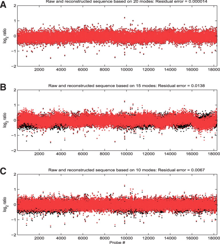
Original (black) and mode-reduced (red) sequences based on 20 (A), 15 (B) and 10 modes (C). Respective residual errors of the reconstructed signals are 1.4e-5, 1.38e-2, 6.7e-3.

To assess the effect of individual modes, signal x(k) may be decomposed into a set of modes that are sequentially eliminated to obtain the m-mode reduced . This is then compared to x(k):

(3)

(4)

where s(k) is the noiseless signal, is the estimate of this signal and ε~N(0, σ_ε²) and w_m~N(0, σ_w²) with σ_wm² < σ_e² are the additive Gaussian noise of the original and reconstructed signals, respectively. The requirement for denoising may be expressed as , i.e. the variance of the estimated signal is less than the variance of the noise in the measured signal. When additional modes are eliminated, the noise variance decreases further, i.e. σ_ε > σ_wm=1 > σ_wm=2 > … >σ_wm=M. However, sequential mode reduction may also eliminate significant components, resulting in large signal reconstruction errors. Thus, we need to bound the number of eliminated modes. We define the risk function as:

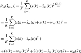(5)

When 0 modes are eliminated from the original signal, and R₀=0. When the reconstructed signal is the optimum estimate of the s(k), then and Equation (5) becomes:

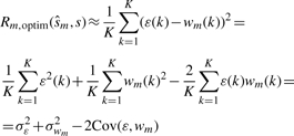(6)

It is assumed that and w(k) are independent and thus . Then, if we set the variance of the mode-reduced signal equal to the risk function, we have [from Equation (6)]

(7)

which ensures the desired (assuming w_m and ε are positively correlated), with equality when ε(k) or w_m(k) is zero, i.e. a noiseless measurement x(k)=s(k) or noiseless estimate and asymptotic equality when K→∞.

There are several threshold estimation approaches for denoising, e.g. wave-shrinkage (Donoho et al., 1994). Although perhaps not optimal, our proposed approach has the advantage of not requiring detailed estimation of the threshold. Setting the variance of the mode-reduced signal equal to the risk function ensures that mode reduction increases SNR. An example is shown in Figure 3, using a subset of the data. Typically, the variance and risk function intersected at mode 1 or 2, depending on the chromosome, and thus 1–2 modes were eliminated.

Fig. 3.

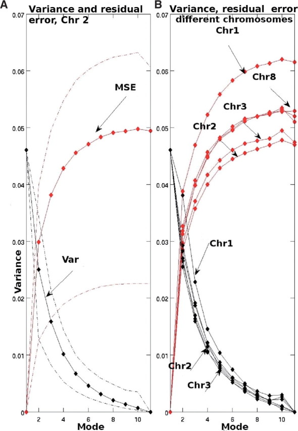
Effects of sequential mode elimination on the risk function (black) and variance (red) of the mode-reduced sequence. (A) The inter sequence parameter variability for one chromosome (dashed lines). Mean parameter values for several chromosomes (B).

We compared the proposed approach to loess curve fitting (Marioni et al., 2007), PCA and ICA. Corresponding changes in SNR (averaged over all sequences) are shown in Figure 4. SNR was computed as the log₂ ratio at each probe divided by the SD of the signal, to be consistent with the definition of SNR in Marioni et al. (2007). Elimination of redundant ICA/PCA components and loess fitting yielded only modest changes in SNR. In contrast, mode elimination resulted in substantial increases in SNR. Similar results were obtained for all chromosomes.

Fig. 4.

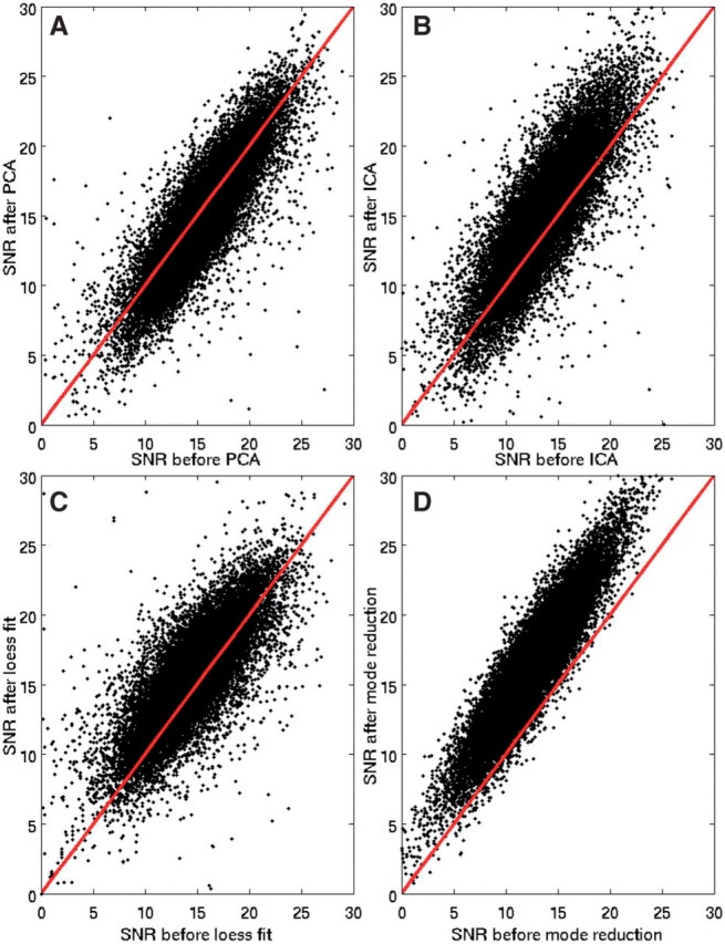
Comparison of artifact elimination via PCA (A), ICA (B), loess curve fitting (C) and mode elimination (D). Each plot is for SNR before (x-axis) versus SNR after application of the respective method (y-axis), averaged over all normal sequences.

3.2 Effect of normalization by a common reference

In addition to the wave-like artifact, a common reference for normalization may also introduce spurious spatial correlations in genomic data. To explore this, the normalization was reversed by adding the log₂ reference to each observed sequence, to obtain non-normalized data:

(8)

where x_i is the non-normalized sequence and x_i,obs the batch-normalized sequence. Each non-normalized sequence was decomposed. Contributions of low-amplitude modes were compared in raw and normalized sequences. The wave-like artifact was not suppressed in non-normalized data, which implies that it is unrelated to the normalization, as also noted in Diskin et al. (2008).

We assessed the effect of renormalization (measured by the variance of the sequence) by renormalizing each sequence by the mean of all others, as shown is Figure 5 (for 20 sequences). The variance of renormalized raw and mode-reduced data were compared. The diagonal entries correspond to the variance of the non-normalized sequence. The effect of normalization was in some sequences significantly higher (~O(1)) than in others, e.g. the variance increase in sequence 1 was negligible when the sequence was normalized by 2–4, 8–14, 18–20, but substantial when normalized by sequences 15–17. In contrast, renormalization of mode-reduced sequences resulted in small variance changes. Thus, denoising via mode elimination reduces the uncertainty associated with normalization by different sequences.

Fig. 5.

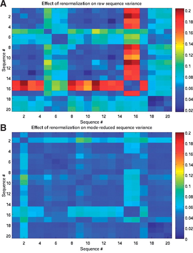
Effect of renormalization on the variance (shown as color) of 20 raw (A) and corresponding mode-reduced sequences (B).

3.3 Matched filtering

Matched filtering is a waveform-matching method that is widely used in pattern recognition, sonar and communications, to detect a desired waveform c(k) in a measured signal x_obs(k). The matched filter is a quasi-optimum filter that locally maximizes the output SNR by decreasing SNR in regions of mismatch between observed and desired (template) signals and increasing SNR in matched regions. It improves SNR by reducing the noise spectral bandwidth to that of the desired waveform (Turin, 1960). Theoretically, the optimum filter that maximizes SNR is the time-reversed signal itself, i.e. c(k)=x_obs(−k) under the assumption of Gaussian noise, and matched filtering is a convolution operation:

(9)

Template signal: typically, the template c(k) is either precisely known or robustly estimated. An observed signal is then matched-filtered with this template. However, in this study there was no unique or known template. Every normal chromosome sequence was treated both as a template and an observation. To identify CNVs, regions of signal mismatch rather than regions of match were examined. Each of N_s mode-reduced sequences was segmented according to the filter length described below, and each of Q segments was filtered with N_s−1 corresponding segments (the templates), to obtain N_s−1 matched-filtered segments. The ratio of pre- over post-filtering SNR ΔSNR, was computed for each segment, and averaged over N_s−1 SNRs. A matrix of ΔSNRs was ultimately obtained of size N_s×Q. A segment was further examined for potential CNVs if , averaged over N_s was less than an estimated threshold, described below.

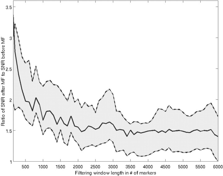
Filter length: the choice of filter length is important for achieving optimal SNR. We examined the change in SNR following matched filtering as a function of filter length. We used the typical definition of SNR = 20 in dB, estimated the change in SNR as , where <·>_rms denotes root-mean squared. Figure 6 shows the average (over all sequences and chromosomes) SNR change as a function of filter length. Since the first change in slope of average SNR change occurs at a length of ~500 probes, which was determined empirically to be sufficiently long for matched filtering, we selected this as the segment/filter length, though it may not be optimal.

Fig. 6.

Ratio of SNR of matched-filtered data over raw data as a function of the filter length. The solid line corresponds to mean SNR change, averaged over all sequence SNRs, and superimposed is the variability of this ratio.

Threshold for estimating regions of mismatch: contrary to the traditional application of matched filtering, for CNV detection we are interested in regions of mismatch rather than regions of maximum match. This is because we presume that CNVs occur with relatively low frequency. Regions of mismatch not only include both allelic variability between two sequences but also potentially distinct noise and artifacts. Thus, the first step of mode decomposition for denoising is necessary. Furthermore, a threshold or random mismatch due to noise rather than true waveform mismatch must also be estimated, instead of assuming that any decrease in SNR, i.e. ΔSNR≤0, following matched filtering reflects waveform mismatch. We simulated and matched-filtered 500 pairs of identical, and thus theoretically perfectly matched signals, but corrupted with distinct additive Gaussian noise sequences, while maintaining high SNR. We estimated that noise-induced mismatch resulted in a maximum decrease in SNR of 1.5 dB. Therefore, regions where mean SNR in the filtered sequence decreased by more than −1.5 dB were identified as regions of potential true waveform mismatch.

CNV call: matched filtering increases/decreases SNR according to match/mismatch, and thus the resulting signal amplitude in the filtered data may be different from the log₂ ratios in the original (but denoised) data. Thus, once potential segments of mismatch have been identified, we need to examine the corresponding segments in the denoised data for determining the actual type of aberration at the probe level. For simplicity, we set a detection threshold of one loss or one gain, i.e. for gain and for loss. The probability of a CNV at probe k was defined as the union of the probabilities of (mutually exclusive) gain and loss. This is practically equivalent to the maximum of these probabilities since one of the probabilities is typically negligible relative to the other:

(10)

where N_s is the total number of sequences, and log₂(j, k) corresponds to the mode-reduced sequence j at probe k. A probability of 0.1 (10% frequency) was chosen as the threshold for a CNV call. Although this choice is somewhat arbitrary, low CNV frequencies ≤10% have been reported in the normal genome (Ionita-Laza et al., 2008; Jakobsson et al., 2008).

4 RESULTS

4.1 CNV detection in the normal genome

We applied SDMF to 429 normal sequences from the TCGA database, and compared them to CNVs in the DGV detected in datasets with least 420 samples, irrespective of their frequency of occurrence, as well as CNVs in two studies with 270 samples and high frequency (≥40%) (McCarroll et al., 2008; Pinto et al., 2007). For the Y chromosome, the maximum sample size in any study was 270. For two CNVs to be comparable, we assumed a very conservative 50% spatial overlap of the length of the detected CNV with respect to the length of the CNV in the DGV. In cases where the same CNV was reported by multiple studies, but with slightly different lengths, the intersection of these regions was assumed as the CNV length. Finally, when a detected aberrations was entirely contained within the genomic coordinates of the corresponding CNV in the DGV, it was called a separate CNV irrespective of its overlap (this occurred in only very few instances). On average, filtering restricted the regions of mismatch for further examination to 19–34% of the total number of segments, depending on the chromosome. This is expected as these were all normal sequences, and thus with high waveform similarities and low mismatch. Table 1 summarizes the number of CNVs in DGV, in each chromosome, irrespective of frequency (column 2); the overall sensitivity of SDMF with respect to DGV, calculated as the ratio of the number of CNVs in the intersection of the two sets over the total number of CNVs in DGV (column 3); Cohen's kappa statistic (Cohen, 1960), as a measure of agreement between SDMF and DGV that accounts for overlap between the two occurring by chance (column 4); CNVs detected by SDMF with least 10% frequency (column 5); CNVs in DGV with at least 10% frequency (column 6); sensitivity of SDMF with respect to CNVs in DGV with frequencies at least 10% (column 7); and the corresponding kappa (column 8). Note that the kappa statistic is calculated at the probe level, by assuming that the maximum number of CNVs is the number of probes in each chromosome. However, CNVs in DGV have been detected with a wide range of arrays of different resolution. To account for this, we obtained the genomic coordinates for each identified CNV in the DGV and calculated the corresponding number of probes in our data, so that the two sets are comparable for the estimation of kappa.

Table 1.

CNVs in DGV (column 2), sensitivity of SDMF with respect to DGV (column 3), κ statistic (column 4), CNVs in DGV and in this study, with at least 10% frequency (columns 5 and 6), sensitivity of SDMF with respect CNVs in DGV with at least 10% frequency (column 7) and the corresponding κ (column 8).

Chr	DGV	Sens. SDMF w.r.t. DGV	κ	SDMF ≥10%	DGV ≥10%	Sens. SDMF w.r.t. DGV>10%	κ10%
1	1235	0.44	0.41	1178	115	0.92	0.15
2	833	0.46	0.46	586	83	0.89	0.21
3	726	0.42	0.5	456	82	0.96	0.29
4	727	0.34	0.38	478	108	0.91	0.32
5	652	0.31	0.32	495	80	0.95	0.26
6	586	0.43	0.4	550	100	0.9	0.27
7	642	0.48	0.56	423	75	0.94	0.27
8	638	0.4	0.4	530	76	0.92	0.22
9	585	0.49	0.54	428	37	0.94	0.14
10	568	0.46	0.47	488	55	0.95	0.18
11	607	0.23	0.28	313	73	0.91	0.33
12	577	0.41	0.42	473	74	0.94	0.25
13	347	0.37	0.4	256	12	0.92	0.08
14	382	0.28	0.33	225	31	0.94	0.2
15	441	0.44	0.54	253	37	0.95	0.23
16	411	0.39	0.42	296	45	0.91	0.23
17	365	0.51	0.57	269	52	0.91	0.28
18	213	0.17	0.25	65	12	0.83	0.26
19	446	0.28	0.32	241	36	0.89	0.22
20	255	0.54	0.58	203	24	0.88	0.18
21	159	0.57	0.67	106	15	0.93	0.22
22	287	0.23	0.35	72	17	1	0.38
X	309	0.59	0.62	267	22	0.91	0.14
Y	27	0.6	0.52	34	2	1	0.11

A significant number of detected CNVs have also been reported in DGV with frequencies ≥10%. For this subset, the sensitivity of SDMF with respect to DGV was ≥83%. The overall sensitivity of SDMF was lower (17–60%). Furthermore, based on the accepted interpretations of levels of kappa (Landis et al., 1977), the agreement between DGV and SDMF was slight (0<κ<0.2) to moderate (0.4<κ<0.6), depending on the chromosome. This may be due due to: (i) differences in the populations of DGV and TCGA normals; (ii) novel CNVs detected by SDMF; and (iii) the use of distinct thresholds for CNV calls in different studies. We can only assess the false positive rate of SDMF through simulations.

4.2 Comparison of SDMF with CBS via simulation

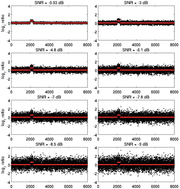
SDMF may be applied to identify regions of mismatch, and thus to detect CNVs occurring at low frequencies in a relatively large set of genomes, or to identify regions of significant waveform match between sequences, and thus to detect common CNVs occurring at high frequencies. We compared SDMF to CBS. Although other methods have been shown to be computationally faster, e.g. Pique-Regi et al. (2008), CBS is widely used for CNV detection (Olshen et al., 2004), by simulating both cases (match/mismatch). The respective performance of the two methods was measured by the true and false detection rates, as a function of SNR and inter-CNV distance. Sequences were corrupted with additive, multiplicative or periodic (sine wave) Gaussian noise. SNR was measured in decibel. We simulated 1000 sequences (100 per each of 10 noise levels). In this set, CNV frequency was 100% and matched filtering was applied in the traditional sense, to identify regions of maximum match between template and test sequences, which corresponded to regions containing CNVs. To simulate low-frequency occurring CNVs, all but 10–25% of sequences in this set were randomly selected and replaced by pure Gaussian noise. An example of a sequence containing 1 short CNV (300 markers long), contaminated with progressively higher additive noise levels (decreasing SNR) is shown in Figure 7. Note that SDMF was applied to simulated data in the same way as in real data, using noise-contaminated sequences as both the template and test signals. All sequences were first mode-decomposed for denoising.

Fig. 7.

Simulated genomic sequences with one CNV and decreasing SNR (0 to −9 dB, top left to bottom right plots), and superimposed original (uncorrupted) sequence (red).

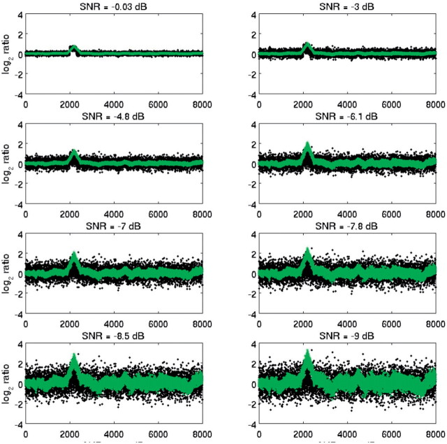
The matched-filtered sequences corresponding to Figure 7 are shown in Figure 8. matched filtering successfully suppressed noise in regions of mismatch, even in very low SNR (−7 to −10 dB), locally increased SNR in the neighborhood of the CNV by at least 5 dB and decreased SNR elsewhere by at least 3 dB. This example demonstrates the ability of SDMF to detect even short CNVs in very high noise levels. Note that when a template with high SNR is precisely known, the first step of signal denoising by mode-reduction results only in modest additional increases in SNR (<2 dB). However, when a robust template is not precisely known and/or is noisy, mode decomposition is a necessary pre-processing step.

Fig. 8.

Individual raw (black) and match-filtered sequences (green).

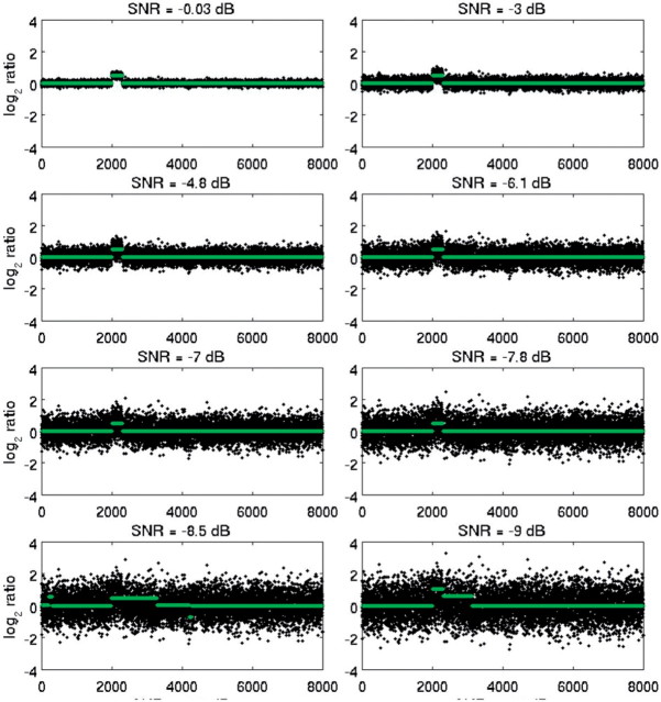
In the examples shown in Figure 9, CBS performed very well for SNR ≥−6dB, but detected spurious CNVs at lower SNRs. In contrast, SDMF correctly identified one CNV in all sequences. In cases of pure noise (no CNVs), neither SDMF nor CBS identified any CNVs. Also, the additional simulations for mismatch did not change the results of CBS, which processes each sequence individually. True and false detection rates of SDMF and CBS as a function of SNR, noise type and distance between CNVs are summarized in Table 2. SDMF correctly detected at least 70% of CNVs irrespective of SNR and noise type, compared with at least 15% detected by CBS. Multiplicative noise decreased the true detection rate in both methods, but periodic noise did not significantly affect detections by SDMF, possibly due to the initial denoising. With regard to inter-CNV distance, for fewer than 1000 markers, SDMF detected 84% of CNVs, versus 40 by CBS, at low SNR. CBS sometimes detected closely spaced CNVs as a single CNV. Also, the estimated mean gain/loss, which depended on the accuracy of the CNV breakpoints, was more precisely estimated by SDMF, particularly for SNR <−6 dB. Finally, false detection rate, estimated as the ratio of falsely identified CNV probes over the number of true non-CNV probes, increased significantly for multiplicative and periodic noise for CBS but not for SDMF. This calculation was based on 8000 probes and a varying number of CNVs of different lengths. In simulations for mismatch, the true detection rate was higher for SDMF than CBS and the false detection rate was lower. As expected, the false detection rate of SDMF in these simulations was slightly higher than the corresponding rate in simulations for waveform match, since it is calculated at the probe level and random mismatch at low SNR may affect the estimated CNV length. In general, although SDMF substantially outperformed CBS at low SNR, CBS performed well for higher SNR. However, the computational cost of CBS was significantly higher (O(5) in simulations and O(8) in real data). Next-generation CGH arrays with very high resolution will require computationally efficient analysis methods. SDMF can handle large genomic datasets, whereas CBS is limited in that respect.

Fig. 9.

Original (black) and CNV detections based on CBS (green).

Table 2.

True and false detection rates for SDMF (S) and CBS (C) as a function of SNR, noise type and simulation type (match/mismatch), and % difference between estimated and true mean log₂ ratio

Parameter	Method	−10	−8	−6	−4	−2
		SNR/Additive noise: Match
True	S	0.84	0.91	0.95	1	1
+ve rate	C	0.42	0.75	0.82	0.95	1
False	S	0.05	0	0	0	0
+ve rate	C	0.42	0.11	0	0	0
Δmean	S	0.01	0	0	0	0
log2 ratio	C	0.2	0.11	0	0	0
		SNR/Multiplicative noise: Match
True	S	0.73	0.85	0.9	0.96	1
+ve rate	C	0.27	0.55	0.64	0.92	1
False	S	0.19	0.15	0.05	0	0
+ve rate	C	0.68	0.36	0.23	0.13	0.1
Δmean	S	0.04	0.02	0	0	0
log2 ratio	C	0.3	0.26	0.1	0	0
		SNR/Periodic noise: Match
True	S	0.8	0.9	0.92	1	1
+ve rate	C	0.17	0.46	0.6	0.84	0.9
False	S	0.11	0.05	0	0	0
+ve rate	C	0.67	0.52	0.45	0.23	0.1
Δmean	S	0.04	0.01	0	0	0
log2 ratio	C	0.35	0.29	0.16	0.09	0
		SNR/Additive noise: Mismatch
True	S	0.83	0.9	0.95	1	1
+ve rate	C	0.42	0.75	0.82	0.95	1
False	S	0.14	0.06	0	0	0
+ve rate	C	0.42	0.11	0	0	0

5 DISCUSSION

We have developed SDMF, a computationally efficient methodology that combines the signal processing tools of signal decomposition and matched filtering for CNV detection in array CGH data. The latter are inherently noisy and robust CNV detection is difficult at low SNR. SDMF treats genomic sequences as spatially continuous, non-stationary signals, which are denoised through elimination of noise-related components. Spatially localized matched filtering is then applied to identify regions of pairwise match/mismatch. Through these two processes, SDMF increases SNR and improves the specificity of CNV detection. Note that SDMF requires the selection of the matched-filter length and thresholds for match/mismatch and loss/gain for CNV detection. These were not explicitly optimized in this study. The choices of filter length and match/mismatch thresholds are dataset dependent. The log2 ratio threshold depends on the goal of the study, e.g. for detection of pathological CNVs it may be based on the log2 ratios of normal CNVs. SDMF was applied to 429 normal sequences from the TCGA, and detected CNVs were compared to those in the DGV. Very high sensitivity (≥83%) relative to the DGV for CNVs with frequency ≥10% was estimated. In simulations, SDMF had a higher true detection rate and significantly lower false detection rate and computational cost than the CBS method, an important advantage when analyzing large datasets from very high-resolution arrays.

In summary, SDMF is a promising approach for CNV detection even in very noisy genomic data. Microarray platforms are rapidly improving and remain the most appropriate tool for interrogating the entire genome at a reasonable cost. Although next-generation sequencing technologies are very promising, their cost currently prohibits the analysis of the entire genome, and may require significant amounts of DNA not always available. Furthermore, there is much information to be gained from existing well-annotated array-based studies through the application of highly sensitive and computationally efficient methods such as SDMF.

REFERENCES

- Alter O., et al. Singular value decomposition for genome-wide expression data processing. Proc. Natl Acad. Sci. USA. 2000;97:10101–10106. doi: 10.1073/pnas.97.18.10101. [DOI] [PMC free article] [PubMed] [Google Scholar]
- Barros A., et al. Assessment of algorithms for high throughput detection of genomic copy number variation in oligonucleotide microarry data. BMC Bioinformatics. 2007;8:368. doi: 10.1186/1471-2105-8-368. [DOI] [PMC free article] [PubMed] [Google Scholar]
- Beckmann J.S., et al. Copy number variants and genetic traits: closer to the resolution of phenotypic to genotypic variability. Nat. Rev. Genet. 2007;8:639–644. doi: 10.1038/nrg2149. [DOI] [PubMed] [Google Scholar]
- Benjamini Y., Hochberg Y. Controlling the false discovery rate: a practical and powerful approach to multiple testing. J. R. Stat. Soc. B. 1995;57:289–300. [Google Scholar]
- Beroukhim R., et al. Assessing the significance of chromosomal aberrations in cancer. Proc. Natl Acad. Sci. USA. 2007;104:20007–20012. doi: 10.1073/pnas.0710052104. [DOI] [PMC free article] [PubMed] [Google Scholar]
- Carter N.P. Methods and strategies for analyzing copy number variation using DNA microarrays. Nat. Genet. 2007;39:S16–S21. doi: 10.1038/ng2028. [DOI] [PMC free article] [PubMed] [Google Scholar]
- Cohen J. A coefficient for agreement for nominal scales. Educ. Psychol. Meas. 1960;20:37–46. [Google Scholar]
- Diskin S.J., et al. Adjustment of genomic waves in signal intensities for whole-genome SNP genotyping platforms. Nucleic Acids Res. 2008;36(e126):1–12. doi: 10.1093/nar/gkn556. [DOI] [PMC free article] [PubMed] [Google Scholar]
- Donoho D., Johnstone I.M. Spatial adaptation by wavelet shrinkage. Biometrika. 1994;81:425–455. [Google Scholar]
- Engler D.A., et al. A pseudolikelihood approach for simultaneous analysis of array comparative genomic hybridization. Biostatistics. 2006;7:399–421. doi: 10.1093/biostatistics/kxj015. [DOI] [PubMed] [Google Scholar]
- Fridlyand J., et al. Hidden Markov Models approach to the analysis of array CGH data. J. Multivar. Anal. 2004;90:132–153. [Google Scholar]
- Huang N.E., et al. Empirical Mode Decomposition and Hilbert spectrum for non-linear, non-stationary time series analysis. Proc. R. Soc. Lond. A. 1998;454:903–995. [Google Scholar]
- Hupe P., et al. Analysis of array CGH data: from signal ratio to gain and loss of DNA regions. Bioinformatics. 2004;20:3413–3422. doi: 10.1093/bioinformatics/bth418. [DOI] [PubMed] [Google Scholar]
- Hsu L., et al. Denoising array-based comparative genomic hybridization data using wavelets. Biostatistics. 2005;6:211–226. doi: 10.1093/biostatistics/kxi004. [DOI] [PubMed] [Google Scholar]
- Iafrate A.J., et al. Detection of large-scale variation in the human genome. Nat. Genet. 2004;39:949–951. doi: 10.1038/ng1416. [DOI] [PubMed] [Google Scholar]
- Ionita-Laza I., et al. On the frequency of copy number variants. Bioinformatics. 2008;24:2350–2355. doi: 10.1093/bioinformatics/btn421. [DOI] [PMC free article] [PubMed] [Google Scholar]
- Jakobsson M., et al. Genotype, haplotype and copy-number variation in worldwide human populations. Nature. 2008;451:998–1003. doi: 10.1038/nature06742. [DOI] [PubMed] [Google Scholar]
- Kallioniemi A., et al. Comparative genomic hybridization for molecular cytogenetic analysis of solid tumors. Science. 1992;258:818–821. doi: 10.1126/science.1359641. [DOI] [PubMed] [Google Scholar]
- Komura D., et al. Genome-wide detection of human copy number variations using high-density DNA oligonucleotide arrays. Genome Res. 2006;16:1575–1584. doi: 10.1101/gr.5629106. [DOI] [PMC free article] [PubMed] [Google Scholar]
- Lai W.R., et al. Comparative analysis of algorithms for identifying amplifications and deletions in array CGH data. Bioinformatics. 2005;21:3763–3770. doi: 10.1093/bioinformatics/bti611. [DOI] [PMC free article] [PubMed] [Google Scholar]
- Landis J.R., Koch G.G. The measurement of observed agreement for categorical data. Biometrics. 1977;33:159–174. [PubMed] [Google Scholar]
- Lupski J.R. Genomic rearrangements and sporadic disease. Nat. Genet. 2007;39:S43–S47. doi: 10.1038/ng2084. [DOI] [PubMed] [Google Scholar]
- McCarroll S.A., et al. Integrated detection and population-analysis of SNPs and copy number variation. Nat. Genet. 2008;40:1166–1174. doi: 10.1038/ng.238. [DOI] [PubMed] [Google Scholar]
- Marioni J.C., et al. Breaking the waves: improved detection of copy number variation from microarray-based CGH. Genome Biol. 2007;8:R228. doi: 10.1186/gb-2007-8-10-r228. [DOI] [PMC free article] [PubMed] [Google Scholar]
- Olshen A.B., et al. Circular binary segmentation for the analysis of array-based DNA copy number data. Biostatistics. 2004;5:557–572. doi: 10.1093/biostatistics/kxh008. [DOI] [PubMed] [Google Scholar]
- Perry G.H., et al. The fine-scale and complex architecture of human copy-number variation. Am. J. Hum. Genet. 2008;82:685–695. doi: 10.1016/j.ajhg.2007.12.010. [DOI] [PMC free article] [PubMed] [Google Scholar]
- Pinto D., et al. Copy-number variation in control population cohorts. Hum. Mol. Genet. 2007:R168–R173. doi: 10.1093/hmg/ddm241. Spec No. 2. [DOI] [PubMed] [Google Scholar]
- Redon R., et al. Global variation in copy number in the human genome. Nature. 2006;44:444–454. doi: 10.1038/nature05329. [DOI] [PMC free article] [PubMed] [Google Scholar]
- Pique-Regi R., et al. Sparse representation and Bayesian detection of genome copy number alterations from microarray data. Bionformatics. 2008;24:309–318. doi: 10.1093/bioinformatics/btm601. [DOI] [PMC free article] [PubMed] [Google Scholar]
- Sebat J., et al. Strong association of de novo copy number mutations in autism. Science. 2007;316:445–449. doi: 10.1126/science.1138659. [DOI] [PMC free article] [PubMed] [Google Scholar]
- Snijders A.M., et al. Assembly of microarrays for genome-wide measurement of DNA copy number. Nat. Genet. 2001;29:263–264. doi: 10.1038/ng754. [DOI] [PubMed] [Google Scholar]
- Turin G.L. An introduction to matched filters. IRE Trans. Inf. Theory. 1960;6:311–329. [Google Scholar]
- Van de Wiel M.A., et al. Smoothing waves in array CGH profiles. Bioinformatics. 2009;25:1099–1104. doi: 10.1093/bioinformatics/btp132. [DOI] [PubMed] [Google Scholar]
- Willett P.K., Thomas J.B. Robust signal selection for the matched filter. IEEE Trans. Signal. Process. 1991;39:2559–2563. [Google Scholar]
- Wineinger N.E., et al. Statistical issues in the analysis of DNA copy number variations. J. Comput. Biol. Drug Des. 2008;1:368–395. doi: 10.1504/IJCBDD.2008.022208. [DOI] [PMC free article] [PubMed] [Google Scholar]
- Zhang F., et al. Copy number variation in human health, disease, and evolution. Annu. Rev. Genomics Hum. Genet. 2009;10:451–481. doi: 10.1146/annurev.genom.9.081307.164217. [DOI] [PMC free article] [PubMed] [Google Scholar]