Comparison of no-prior and soft-prior regularization in biomedical microwave imaging

Abstract

Microwave imaging for medical applications is attractive because the range of dielectric properties of different soft tissues can be substantial. Breast cancer detection and monitoring of treatment response are areas where this technology could be important because of the contrast between normal and malignant tissue. Unfortunately, the technique is unable to achieve the high spatial resolution at depth in tissue which is available from other conventional modalities such as x-ray computed tomography (CT) or magnetic resonance imaging (MRI). We have incorporated a soft-prior regularization strategy within our microwave reconstruction algorithm and compared it with the images obtained with traditional no-prior (Levenberg-Marquardt) regularization. Initial simulation and phantom results show a significant improvement of the recovered electrical properties. Specifically, errors in the microwave property estimates were improved by as much as 95%. The effects of a false-inclusion region were also evaluated and the results show that a small residual property bias of 6% in permittivity and 15% in conductivity can occur that does not otherwise degrade the property recovery accuracy of inclusions that actually exist. The work sets the stage for integrating microwave imaging with MR for improved resolution and functional imaging of the breast in the future.

Introduction

Microwave imaging (MI) for biomedical applications is based on recovering the electrical properties (permittivity and conductivity) of tissue. Early studies showed a significant dielectric property contrast between normal and malignant breast tissues;[1–3] however, more recent data have indicated that the properties of the normal breast are more variable than originally thought and that the contrast may not be as great for some types of breast tissue.[4] This is particularly true for radiographically denser breast with higher concentrations of fibroglandular tissue.[4] Notwithstanding, early clinical MI studies on patients with suspected tumors have demonstrated significant discrimination between those with malignant cancers versus those with benign lesions and other normal tissues.[5] In addition, the non-ionizing and non-compressive nature of MI makes the technique potentially attractive for cancer screening.[6]

MI mainly consists of solving two problems: the forward problem and the inverse problem. The forward problem involves computing the output (i.e., the scattered field) from known inputs (i.e., the low-power, non-ionizing microwave exposure) and system properties (i.e., the dielectric property distribution of the tissue being imaged), whereas the inverse problem estimates the properties of an unknown volume (i.e., the dielectric properties of the tissue) from known input (i.e., the low-power, non-ionizing microwave exposure) and measured field values. Since the inverse electromagnetic problem is non-linear, the image reconstruction process is solved iteratively.[7,8] Moreover, because of its ill-posed nature Gauss-Newton schemes are well suited to the application but require some form of regularization to impose additional constraints.[8] Although regularized Gauss-Newton methods can be susceptible to convergence to local minima, we have found that log transformationserves to mitigate these effects.[9,10] Indeed, recent studies of convergence indicate that our Gauss-Newton algorithm reaches the same image (i.e., solution) for widely different initial estimates suggesting that it is not easily trapped by local minima.[11] Completely different approaches to inverse problem solution such as genetic algorithms and stochastic processes are also possible and have been applied successfully to MI as well.[12–14]

Regularization may also involve a priori information about the tissue being imaged, which can be necessary to ensure convergence of the reconstruction algorithm to the correct electromagnetic property distribution.[15] In MI applications, a number of studies have investigated the incorporation of different types of priors ranging from the internal and/or external shape of the body to information about tissue dielectric properties including their upper and lower bounds.[16–25] For example, Crocco et al assumed that the object was homogeneous and that the permittivity value of the target was known.[26] In their shape reconstruction simulation study, El-Shenawee et al, used estimates of inclusion properties and location, and exact knowledge of the number of targets to aid convergence to a viable solution.[27]

Soft-prior regularization can be used to combine the functional information available through MI (i.e. property contrast) with the high spatial resolution of MR or x-ray CT to recover more accurate dielectric properties. The spatial prior is considered “soft” because it does not force the property estimates inside an identified region to be constant. Rather, the known boundary data are used to adjust the regularization to smooth the property estimates within a pre-defined region but not across its boundaries (to preserve property changes at its interface with other tissues). The approach has been developed successfully in a similar imaging system that represents a combination of NIR tomography and MRI methods for breast cancer detection.[28]

In this investigation, we develop the analogous image reconstruction strategy for MI that exploits structural information as a soft-constraint in the microwave property estimation process and compare its performance with a standard no-prior (Levenberg-Marquardt) regularization. The soft-prior algorithm encodes spatial information from different regions of the tissue being imaged into a regularization matrix that associates points within the same region of the reconstruction mesh to minimize variation within each zone. The focus of the study is to evaluate quantitatively the accuracy of the microware property estimates recovered with and without soft-prior regularization in a series of simulation and phantom experiments including under conditions of false inclusions. While MI studies published in the literature have considered priors in various forms, the spatially encoded regularization matrix used here has not been previously implemented or otherwise systematically evaluated when applied to property estimation governed by the time harmonic wave equation. Further, the property accuracy improvements observed with the approach when used with MI phantom data offer the first evidence that the technique produces quantitatively superior results under experimental conditions.

Breast MR is widely used clinically and despite pressures from healthcare cost containment, the number of breast MR imaging studies is likely to continue to grow in the future because of their exquisite soft tissue delineation. However, breast MR has a substantial false positive rate for cancer.[29] As a result, significant opportunities exist to supplement the diagnostic information derived from MR with another modality such as co-registered MI which may be used as complementary image data to improve the specificity of breast MR, especially if the MI properties in areas of contrast enhancement can be accurately estimated. Indeed, this same soft-prior technique resulted in a 26% decrease in the root mean square (RMS) error of the absorption and reduced scattering coefficient images when prior structure of a phantom was used to guide the NIR property estimation[30] and the prospect of attaining similar positive results with MI has motivated the algorithm development and evaluation described here.

Materials and Methods

Image reconstruction without priors

Reconstruction algorithms in MI are based on determining the distribution of the constitutive parameters within tissue where the dielectric properties are embedded in a constitutive equation involving the squared complex-valued wave number which can be written as

where is the position vector in the imaging domain, ω is the angular frequency, j is the imaginary unit, μ₀ is the free-space permeability, ε is the permittivity, and σ is the conductivity. In our algorithm, calculation of the forward solution is based on the 2D form of Maxwell's equations and is computed using a finite difference time domain (FDTD) algorithm,[31] whereas the reconstruction process is based on a Gauss-Newton iterative approach with a variance stabilizing transformation in which the measured electric field vector, , is matched iteratively with the computed electric field vector, , calculated using the forward model for a given distribution of the constitutive parameters stored in the vector k².[9,32] In the 2D FDTD method, a frequency domain field response is produced for each transmitter and the individual field values are extracted at each receiver location.[33] The length of the vector k² is N, the number of reconstruction parameters. In order to overcome the ill-posedness of the problem, constraints on the reconstructed image are required. In our algorithm, Tikhonov regularization[8] is used to stabilize the reconstruction procedure, albeit with added smoothing. The objective function is

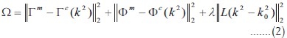
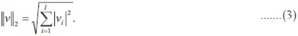
whereand Γ^c are Γ^c the log magnitudes and Φ^m and Φ^c are the phases of the measured and computed field values, respectively,[9,32,33] λ is the weighting coefficient, also known as the Tikhonov regularization parameter, and L is a positive definite, dimensionless regularization matrix. k₀² is a prior estimate of k² and the two-norm of a vector of length O (in this case O is the number of measurements)is the square root of the sum of the squares of the complex modulus of its elements:

In our previous and current studies, the choice of λ is derived empirically. After some manipulation, equation 2 can be solved for the iterative property update, Δk_η²

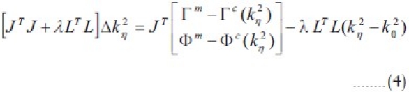
where J is the Jacobian matrix, which has dimensions 2O × 2N and consists of derivatives of the log magnitude and phases of the computed field values with respect to the property values at each of the N reconstruction parameter mesh nodes. k_η² is the vector k² at iteration η and is updated as

This implementation is referred as a Gauss-Newton iterative algorithm with a variance stabilizing transformation.[10,33] In addition, a dual-mesh approach is used where the forward solution is computed on a rectangular uniform FDTD lattice, while the electromagnetic property parameters are reconstructed on a triangular element mesh placed concentrically within the antenna array.

In our original reconstruction algorithm, the regularization matrix L in equation (4) was set to the identity matrix, which applied the same weight to the values at all nodes within the imaging domain. In addition, k₀² was set to leading to k_η² a simplified version of the update equation:

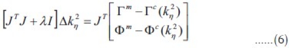
corresponding to the Levenberg-Marquardt algorithm.[7]

Soft-prior encoding of spatial information

We have modified our reconstruction algorithm based on the update equation (6) to include prior spatial information on the boundaries within the tissue (or phantom) being imaged following the methods reported in.[28,30,34–36] Soft- prior regularization penalizes the variation within regions that are assumed to have the same or similar dielectric properties. In addition, when two different regions share the same boundary, the smoothing across their common interface is restricted.[30] In the current implementation, we incorporate prior information about the structure of tissue through the regularization matrix, “L”, in the update equation (4). According to information known about the tissue's structure (derived from a high spatial resolution source such as MR images), each node in the reconstruction mesh is assigned a region number. Given two nodes, i and j, in the reconstruction mesh with their associated regions, R_i and R_j, the corresponding entry in the L matrix is defined as

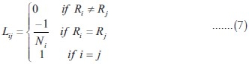
where N_i is the number of nodes in region R_i. Based on this construction of L, L^TL in equation (4) approximates a second-order Laplacian smoothing operator inside each region, which limits the smoothing across the boundaries of distinct regions.[37,38] Since the structure of the tissue being imaged does not change during the iterative image reconstruction algorithm, both the regularization matrix L and Laplacian smoothing operator L^TL, can be calculated once and stored at the beginning of the procedure to avoid redundant calculations (making the algorithm more efficient).

Imaging system

In order to evaluate the soft-prior implementation relative to the no-prior case based on actual measured data from phantom experiments, we have used our prototype breast imaging system for data acquisition. The imaging array consists of 16 monopole antennas located on a 15.2 cm diameter circle. The coupling liquid comprises an 86:14 glycerin:water mixture that is sufficiently lossy at these frequencies to attenuate unwanted reflections from the tank walls and base. The operating frequency ranges from 500 MHz to 3.0 GHz. Each channel operates in both transmit and receive modes at a single frequency which is serially scanned over a user-defined band (e.g. from 1100 to 1700 MHz) at a user-specified increment (e.g. 100 MHz) depending on the measurement data of interest. The antennas sequentially transmit a signal, while the other 15 act as receivers. As a result, 240 (16 transmitter × 15 receivers) measurements of the scattered field are obtained at each frequency and used in the reconstruction process. The measured field component at each receiver is parallel to the axis of the antenna array representing a transverse magnetic (TM) polarization which is assumed during the 2D image reconstructions reported here. A more complete description of our clinical imaging system can be found in Meaney et al.[39]

Error analysis

Since the true values of the dielectric property distribution are known in simulations and phantom experiments, the relative error between the true property distribution and the estimated values can be computed as

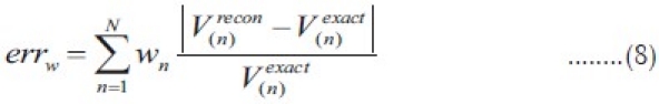
where V_(n)^recon is the reconstructed dielectric property value (either permittivity or conductivity) at node n (in the reconstruction mesh), whereas V_(n)^exact is the true value of the selected dielectric property at that location. To account for the fact that nodes in the reconstruction meshes are not uniformly distributed, a weighting factor has been added at each location computed as w_n = A_n/A, where A_n is the area of the elements surrounding node n and A is the total imaging area. Because of the iterative nature of the reconstruction procedure, a stopping criterion is needed to terminate the algorithm. Since the algorithm typically converges within 15 iterations, we allowed all reconstructions to execute for 20 iterations as a simple way to ensure convergence in each case and verified that the squared error (i.e. equation (2)) was below a threshold (relative to the squared error produced by the initial estimate) of 0.2 in each case.

Results

In the current study, we evaluated MI with soft-prior regularization relative to MI with no priors in simulation and phantom experiments where the boundaries of different regions were known. Figure 1 shows a schematic of the imaging geometries considered. The “Simulation Results” section reports simulations involving variations in mesh resolution and synthetic measurement noise. The effects of parameter coupling and arbitrary inclusion geometry are also investigated. The “Phantom Experiments” section describes analogous results from phantom experiments which consider the impact of false inclusions as well.

Figure 1.

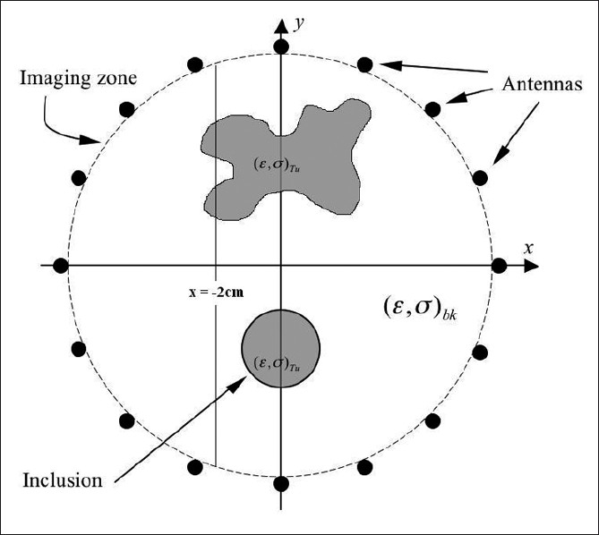
Schematic of the imaging domains evaluated. The background diameter was 14 cm (antennas are positioned on a 15.2 cm diameter). The circular inclusion's center with radius r = 1.40 cm was located at (0,–3 cm), whereas the arbitrarily shaped inclusion was located in the upper part of the imaging domain. The reconstructed values from the simulation experiment with an here arbitrarily shaped inclusion were extracted at 30 points evenly distributed along the line x = –2 cm

Simulation results

Simulated measurement data were generated by our hybrid boundary element/finite element approach[40] for the circular target shape in Figure 1. The images were reconstructed at 1300 MHz using update equation (6) with no spatial information (on reconstruction parameter meshes with 473, 915, 961, and 1725 nodes), and update equation (4) with the soft-prior regularization defined in equation (7) (on the 915 and 1725 node meshes which had external and internal boundaries conforming to the outer surface and lower circular inclusion in Figure 1).

Mesh resolution and noise level

The cylindrical inclusion centered at (x,y) = (0,–3 cm) with a radius of 1.4 cm and the dielectric properties of ε_r,Tu = 51.16 and σ_Tu = 1.44 S/m was embedded in a background medium with the dielectric properties of ε_r,bk = 15.60 and σ_bk = 0.90 S/m. Noise ranging from –110 dBm to –80 dBm was added to the synthetic measurements. Figure 2 shows reconstructed images at 1300 MHz (noise level of –100 dBm) using the no prior (on 473, 915, and 961 node meshes) and soft-prior (on the 915 node mesh) regularizations, respectively. Without spatial priors, the reconstructed images are very similar which indicates that increasing the number of nodes or changing their distribution to be preferentially greater within the inclusion in the reconstruction mesh does not improve the quality of the recovered images. Both regularizations recovered the inclusion in the permittivity and conductivity images, but those from the soft-prior technique are more accurate in terms of the recovered property values. In addition, the recovered background permittivity and conductivity values are more uniform in the soft-prior case. Figure 2 confirms that these improvements are not due to the reconstruction mesh, but to the regularization matrix. The weighted permittivity and conductivity errors without priors were 0.172 and 0.128, respectively, while those with soft-prior regularization were reduced by nearly a factor of 8 to 0.028 and 0.016, respectively.

Figure 2.

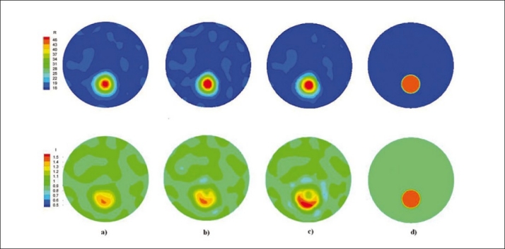
Simulated 1300 MHz reconstructed permittivity (top) and conductivity (bottom) images (a) without priors on the 473 node mesh, (b) without priors on the 961 node mesh, (c) without priors on the 915 node mesh with preferential node deployment in the inclusion, and (d) with soft-prior regularization on the 915 node mesh.

In order to compare the reconstructed and the true dielectric properties, vertical transects of the permittivity and conductivity profiles along the y-axis are shown in Figure 3, for added noise levels of –110, –100, –90, and –80 dBm. In this case, the measurements ranged in amplitude from –30 dBm for the nearest antennas to –87 dBm for those farthest away from the transmitter. The signal to noise ratio for the lowest amplitude measurements with –80 dBm of added noise was 7 dB. As expected, artifacts increased in both the permittivity and conductivity images without priors as the noise level rose, especially in the –80 dBm conductivity images where the fluctuations are significant. The soft-prior regularization tolerates the added noise much better with relatively minor decreases in the recovered inclusion permittivity and only slightly greater reductions in conductivity at the highest noise level. Using soft-priors, the reconstructed permittivity values were underestimated (~10--15%) in the inclusion at all noise levels. Notwithstanding, the method clearly detected the inclusion given the large property contrast with the background. In addition, even when considerable noise was added to the measured data (–90 dBm), the algorithm with soft-prior regularization recovered the inclusion conductivity very accurately, and started to underestimate (~15%) its property values only at even higher noise levels (–80 dBm).

Figure 3.

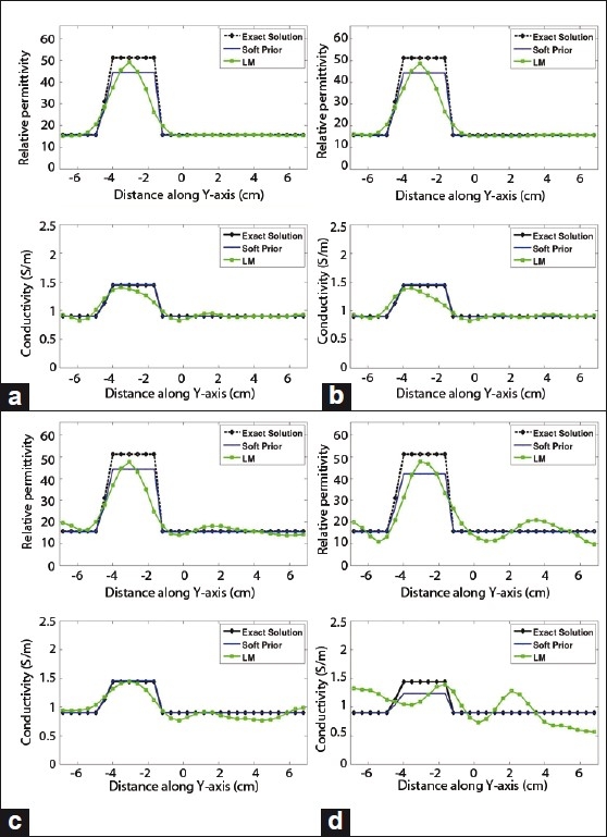
Comparison of the 1300 MHz reconstructed permittivity (top) and conductivity (bottom) values using no-prior (Levenberg-Marquardt, LM) and soft-prior regularizations with different levels of added noise: (a) –110, (b) –100, (c) –90, (d) –80 dB m.

Estimation parameter coupling

In order to study the effects of no prior and soft-prior regularization on reconstruction parameter coupling, two simulation experiments were performed in the same background medium (ε_r,bk= 15.60 and σ_bk = 0.90 S/m). In the first case, no permittivity contrast existed in the inclusion region (dielectric properties were ε_r,Tu=15.60 and σ_Tu = 1.44 S/m). The second experiment had no conductivity contrast in the inclusion (dielectric properties were ε_r,Tu = 51.16 and σ_Tu = 0.90 S/m). Figure 4 shows transects of the 1300 MHz reconstructed permittivity (top row) and conductivity (bottom row) profiles along the y-axis for the first and second experiments (in the left and right columns of the composite figure), respectively (with added noise of –100 dBm).

Figure 4.

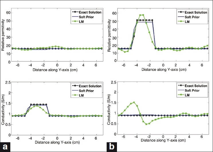
Comparison of 1300 MHz reconstructed permittivity (top row) and conductivity (bottom row) profiles for the no-prior (Levenberg- Marquardt, LM) and soft-prior regularizations: (a) no permittivity contrast (left column), (b) no conductivity contrast (right column)

While both methods (no-priors and soft-priors) handle the no-permittivity contrast case [Figure 4a] effectively, the soft-prior regularization is clearly superior when no conductivity contrast exists in the inclusion [Figure 4b]. The soft-prior regularization profile almost overlaps the exact solution, whereas the no-prior regularization curve has significant differences with the exact solution. Quantitatively, the permittivity--conductivity parameter coupling is only about 5% with the soft-prior regularization in both Figure 4 cases. Here, we consider the permittivity--conductivity parameter coupling to be the relative error (equation 8) between the true values and the recovered properties in the region of the inclusion in the no-contrast images (i.e., reconstructed permittivity in the inclusion in Figure 4a (top row, left column) and conductivity in Figure 4b (bottom row, right column)) when using the soft-prior regularization.

Arbitrarily shaped inclusion

An arbitrarily shaped inclusion [Figure 1] with the dielectric properties of ε_r,Tu = 40.0 and σ_Tu = 1.30 S/m was embedded in a background medium with the dielectric properties of ε_r,bk = 15.60 and σ_bk = 0.90 S/m. With the addition of –100 dBm of noise to the data, the images were reconstructed at 1300 MHz both with and without priors, as shown in Figure 5. Figure 6 shows transects of the reconstructed permittivity (left) and conductivity (right) profiles along the line x = –2 cm using the two regularizations along with the exact solution. While the LM regularization images show an object at roughly the correct location, both the permittivity and conductivity component of the soft-prior images recover the complex shape and properties exactly. In addition, the level of artifacts in the background is significantly reduced with this approach.

Figure 5.

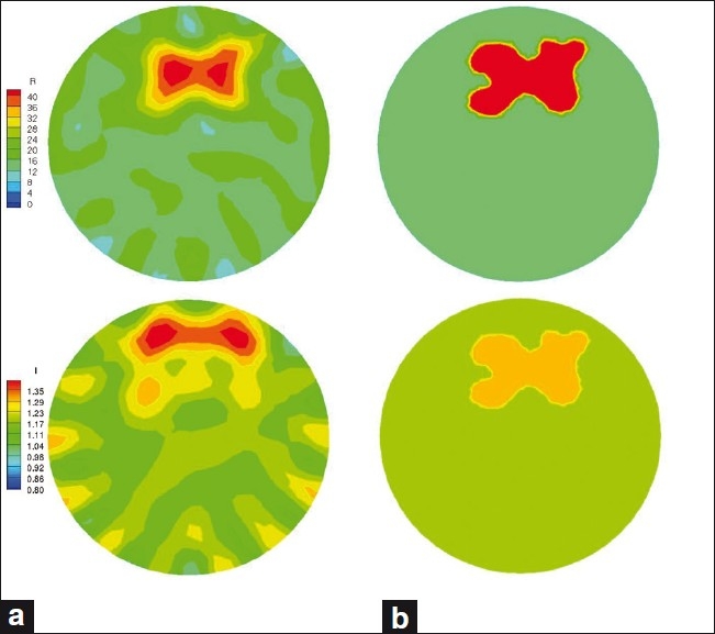
1300 MHz reconstructed permittivity (top) and conductivity (bottom) images from a phantom experiment with arbitrarily shaped inclusion for (a) no-prior and (b) soft-prior regularizations

Figure 6.

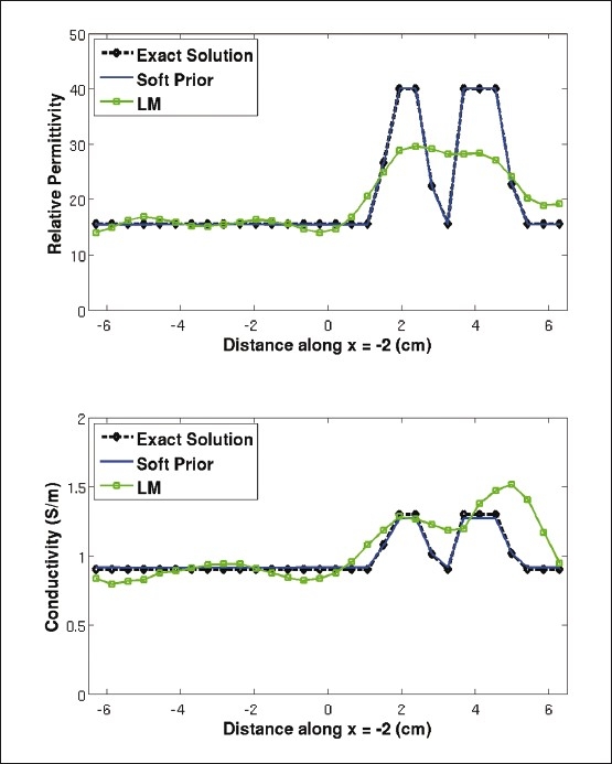
Comparison of the 1300 MHz reconstructed permittivity (top) and conductivity (bottom) profiles along the line x = –2 cm in the figure 5 experiment with arbitrarily shaped inclusion for the no-prior (LM) and soft-prior regularizations

Phantom experiments

In order to illustrate differences in no-prior and soft-prior regularization of experimental data, several phantom experiments were performed at 1100, 1300, 1500, and 1700 MHz. The geometry used in this study was the same as the simulations with the circular inclusion described in the “Mesh Resolution and Noise Level” section. Specifically, a 1.4 cm radius, thin-walled plastic cylinder filled with a mixture of 55% glycerin and 45% water was offset along the y-axis in the background medium (86:14 glycerin:water mixture) by 3 cm.

No-Prior versus soft-prior regularization

Figure 7 shows the images obtained with the two regularizations. In both instances, the inclusion is evident. Several background artifacts appear in the no-prior images, which are more pronounced in the conductivity parameter. Incorporating thespatial priors substantially improves the quality of both the permittivity and conductivity images. Weighted permittivity and conductivity errors decrease from 0.329 and 0.302 to 0.015 and 0.045, respectively, when the spatial structure of the phantom is incorporated through soft-prior regularization. Figure 8 shows the reconstructed dielectric properties from the two approaches along the y-axis relative to the exact values.

Figure 7.

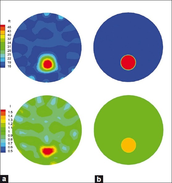
1300 MHz reconstructed permittivity (top) and conductivity (bottom) images from a phantom experiment for (a) no-prior and (b) soft-prior regularizations

Figure 8.

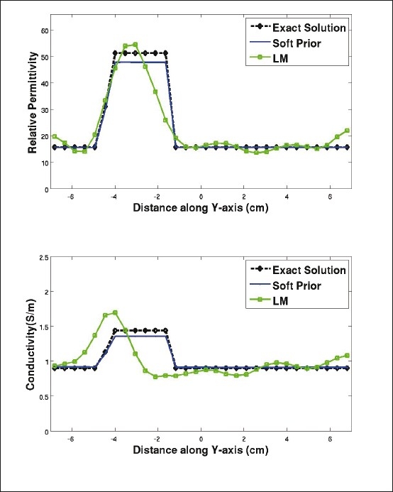
Comparison of the 1300 MHz reconstructed permittivity (top) and conductivity (bottom) profiles along the y-axis in the figure 7 phantom experiment for no-prior and soft-prior regularizations

Clearly, the soft-prior regularization dramatically reduces the spatial oscillations within the background, but it also recovers the dielectric properties in the inclusion more accurately. Improvements are even more pronounced in the conductivity images in which case the recovered inclusion values are over-estimated and displaced (toward the boundary) without priors. These artifacts are eliminated when the spatial structure of the phantom is incorporated through soft-prior regularization.

Choice of soft-prior coefficient

In all previous results, the soft-prior coefficient, λ in equation 4, was set to unity as a default, but in this section, a more detailed study of the effects of λ as a function of frequency is presented. Data from the same experimental setup described in the “No-Prior versus Soft-Prior Regularization” section was used and images were reconstructed at 1100, 1300, 1500, and 1700 MHz. The independently measured dielectric properties of the coupling medium and the inclusion are reported in Table 1 as a function of frequency. A spectrum of soft-prior coefficients was used for the reconstruction procedure, λ = 0.01, 0.1, 1, 10, and 100, based on testing over an even wider range of values in simulation and phantom experiments. Lower values, such as 0.001 for λ, allowed the solution to diverge in some cases, while higher values tended to suppress the recovered inclusion properties. Transects along the y-axis of the reconstructed images for ε_r and σ at 1100, 1300, 1500, and 1700 MHz for the range of soft-prior coefficients are shown in Figure 9. The weighted permittivity and conductivity errors associated with each image are computed and summarized in Table 2. In general, no observable difference occurred between the reconstructed values when λ=1.0 and λ=10. When λ=0.01 the recovered properties in the inclusion are close to the exact values, whereas those of the background begin to deviate from the true levels at higher frequencies. The λ=100 reconstructions appear to estimate the inclusion conductivity values closer to the true levels than the corresponding permittivities which are noticeably underestimated. The weighted property errors are elevated at all frequencies by an order of magnitude when compared to the two lower λ cases. These results suggest that values in the range of λ=1.0 and λ=10 appear to be appropriate soft-prior weighting coefficients over our reconstruction frequency range (usually from 1100 to 1700 MHz). However, the stability of the weighting parameter λ investigated here is based on the present set of experiments, and other situations, for example, with multiple inclusions or different contrast levels may lead to different results and should be investigated further in the future.

Table 1.

Independently measured dielectric properties of the background medium and inclusion over the range of frequencies evaluated

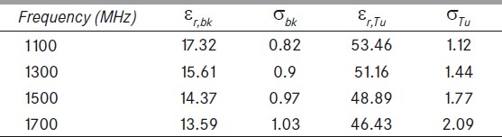
Figure 9.

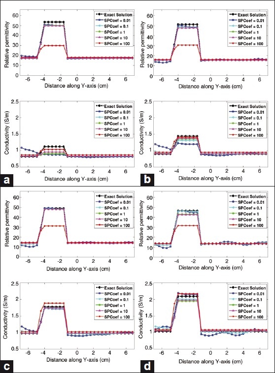
Comparison of the reconstructed permittivity (top), and conductivity (bottom) values from phantom experiment for different values of the spatial prior coefficient, λ, at (a) 1100, (b) 1300, (c) 1500, and (d) 1700 MHz, respectively

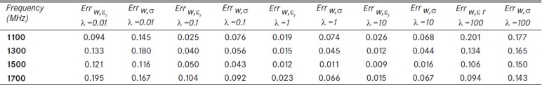
Table 2.

Weighted ε_r and σ errors for a phantom experiment over a range of frequencies from 1100 to 1700 MHz using five different soft-prior coefficients: λ =0.01, 0.1, 1, 10, and 100.

Sensitivity to false inclusions

The behavior of soft-prior regularization in regions, which are identified prior to MI property estimation but do not actually have contrast, is of interest because of the potential of the approach to identify false inclusions based solely on the presumed structural information. Figure 10 shows a reconstruction mesh with a false inclusion region (radius of 1.4 cm) centered at (0, 3cm) along with the previous target zone [Figure 1]. We used the same measurement data generated in the phantom experiments described in the previous section, where only a single inclusion at the lower location (0, -3 cm) actually existed.

Figure 10.

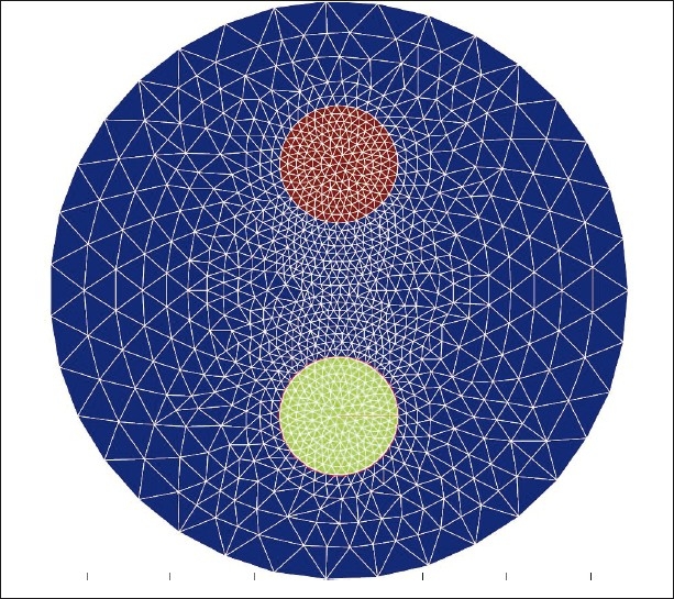
Reconstruction mesh (1196 nodes and 2215 elements) with a false inclusion (upper circle)

Figure 11 shows the 1300 MHz reconstructed images when λ=0.01, λ= 0.1 and λ=1.0, respectively. The false region appears as a weak increase (~ 3 to 6%) in the permittivity images, but with a more pronounced decrease (~ –4% to –20%) in the conductivity images. Transect plots through the inclusion in the permittivity and conductivity images are presented in Figure 12. Consistent with the images in Figure 11, the permittivity values within the false inclusion region are close to the true background, while the conductivity profile is more noticeably affected and exhibits lower values than the background liquid, especially when larger values of λ are used. Since the contribution from the soft-prior regularization is reduced when λ=0.01, the dielectric properties are not significantly influenced by the presence of the false inclusion region (~ 3% and ~ –4% error in the permittivity and conductivity images, respectively). However, for smaller values of λ, more artifacts are observed in the background. As the soft-prior weighting coefficient increases to λ=1.0, more error appears in the false inclusion region (~ 6% and ~ –20% in the permittivity and conductivity images, respectively). The weighted errors are reported in Table 3. For λ=1, err_w,εr = 0.131 and err_w,σ = 0.162, which are larger relative to the case when the exact spatial structure of the phantom was used (err_w,σ = 0.015 and err_w,σ = 0.045), but significantly lower than those obtained without priors (err_w,σr = 0.329 and err_w,σ = 0.302).

Figure 11.

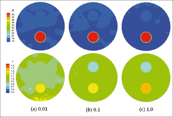
1300 MHz reconstructed permittivity (top) and conductivity (bottom) images of a phantom experiment using soft-prior regularization and the reconstruction mesh with a false inclusion region shown in Figure 10

Figure 12.

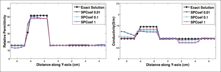
1300 MHz reconstructed permittivity (left) and conductivity (right) profiles from a phantom experiment using soft-prior regularization and the reconstruction mesh with a false inclusion region shown in Figure 10

Table 3.

Weighted ε_r and σ errors for a phantom experiment using the soft-prior regularization and the reconstruction mesh with a false inclusion region for three different soft-prior coefficients: λ =0.01, 0.1, and 1.0 at 1300 MHz

Discussion

We have shown that reconstructed images using simulation and measurement data with soft-prior constraints significantly improve the accuracy of the recovered dielectric properties compared with no prior regularization. We also confirmed that this improvement is not due to the number or distribution of nodes in the reconstruction mesh, but to the regularization matrix which incorporates structural priors into the reconstruction procedure. The weighted errors for the simulated 1300 MHz images with –100 dBm noise decreased by 83% and 87% for ε_r and σ , respectively, when the soft-prior regularization was used. Comparable error reductions of 95% and 85% were observed when using actual measurement data. Moreover, soft-prior regularization is considerably more robust in the presence of noisy data and an arbitrary-shaped inclusion, and is also able to dampen estimation parameter coupling effects, especially in the conductivity, much more readily than Levenberg-Marquardt regularization without spatial information.

We also studied the range over which the soft-prior coefficient was optimal and the algorithm's behavior outside of this span. For a wide operating frequency range (1100 to1700 MHz), λ =0.1 to λ =10 produced similar high quality reconstructions with lower values causing divergence and higher values producing overly smoothed images. In the latter case, the recovered properties of the inclusion dropped significantly from the actual values to levels closer to the background.

Finally, the sensitivity of the soft-prior approach to false inclusion regions was analyzed when using experimental phantom data. The results indicate that creating a false inclusion region and weighting it with the soft-prior regularization does introduce some bias, especially for larger weighting coefficients. For these experiments, the effect observed was a modest increase of 3--6% in permittivity and a more pronounced decrease in conductivity (~–4% to –20%) compared to the surrounding background. Overall, the deviations were relatively minor, and did not detract from the net benefit of improved property recovery in the true target zone. However, the false inclusion evaluated in the “Sensitivity to False Inclusions” section represents a simple example of an extreme case of imperfect shape and location of a region. The behavior of the algorithm when small errors occur in an actual inclusion boundary is an important consideration that warrants further investigation. Our initial results indicate that the MI property estimates deviate smoothly from the true values as location and shape errors increase, but a thorough study of the impact of true-inclusion boundary errors remains to be reported in the future. The occurrence of multiple inclusions, each potentially with its own contrast (that might prove to be true or “false”), has also not been studied, but is likely to occur during clinical imaging and needs to be understood as the MI soft-prior algorithm is refined and developed further.

Since we have adapted methods for introducing spatial priors that have already been developed for NIR tomography, it is interesting to compare the general performances of soft-prior regularization with the two forms of data. Both imaging methods utilize model-based image reconstruction where the properties to be estimated depend nonlinearly on the measurements, but the NIR problem is governed by a time-harmonic diffusion equation whereas the microwave problem obeys a time-harmonic wave equation. No doubt the spatial priors dramatically improve the quantitative accuracy with which the respective image properties can be recovered with the two imaging systems. However, a striking difference occurs in the degree to which a false inclusion manifests itself and the amount of reconstruction parameter coupling that can result. In the NIR case, the contrast and coupling effects (on a true inclusion) of the false inclusion are much more significant than in the corresponding microwave reconstructions where very modest influences were observed.[41] Additionally, the independence with which contrast in permittivity is recovered relative to conductivity; that is, the degree of estimated property parameter coupling is much less in the microwave case when spatial priors are invoked relative to the equivalent NIR problem where property parameter coupling is fairly significant (anywhere from 15% to 40% or more depending on noise level[28,38] compared to about 5% here). While these observations and assessments of the encoding of spatial priors favor the outcomes attained with MI (relative to NIR), some caution is advised not to over-interpret the results (e.g. in terms of property parameter coupling and the effect of false inclusions) because quantitative evaluations must be carefully controlled (e.g. in terms of contrast, inclusion size, location, etc) in order to represent a fair comparison between the two imaging techniques.

Finally, the choice of 1/ N_i as the weighting factor in equation (7) has not been optimized or extensively evaluated and other options are certainly possible. For example, since the elements in the reconstruction parameter mesh comprise different areas, a region-specific, area-related weighting factor might improve performance and is well worth exploring in the future.

Conclusions

We have compared no-prior (Levenberg-Marquardt) versus soft-prior regularization in microwave image reconstruction under a series of representative circumstances. The findings have been supported by simulation and phantom results which indicate that including structural information in the form of a soft-constraint can significantly improve the recovered images both qualitatively and quantitatively. The implementation of soft-prior regularization is appealing because it demonstrates that current measurement data sets are sufficient (in combination with anatomical knowledge) to produce high fidelity reconstructions of experimental phantom targets which is an encouraging first step. The framework presented here sets the stage for extending the approach to more complex 2D and 3D phantom experiments and eventually to clinical patient data where anatomical images might be available from other modalities such as MR.

References

- 1.Chaudhary SS, Mishra RK, Swarup A, Thomas JM. Dielectric properties of normal & malignant human breast tissues at radiowave & microwave frequencies. Indian J Biochem Biophys. 1984;21:76–9. [PubMed] [Google Scholar]
- 2.Joines WT, Zhang Y, Li C, Jirtle RL. The measured electrical properties of normal and malignant human tissues from 50 to 900 MHz. Med Phys. 1994;21:547–50. doi: 10.1118/1.597312. [DOI] [PubMed] [Google Scholar]
- 3.Surowiec AJ, Stuchly SS, Barr JB, Swarup A. Dielectric properties of breast carcinoma and the surrounding tissues. IEEE Trans Biomed Eng. 1988;35:257–63. doi: 10.1109/10.1374. [DOI] [PubMed] [Google Scholar]
- 4.Lazebnik M, Popovic D, McCartney L, Watkins CB, Lindstrom MJ, Harter J, et al. A large-scale study of the ultrawideband microwave dielectric properties of normal, benign and malignant breast tissues obtained from cancer surgeries. Phys Med Biol. 2007;52:6093–115. doi: 10.1088/0031-9155/52/20/002. [DOI] [PubMed] [Google Scholar]
- 5.Poplack SP, Tosteson TD, Wells WA, Pogue BW, Meaney PM, Hartov A, et al. Electromagnetic breast imaging: results of a pilot study in women with abnormal mammograms. Radiology. 2007;243:350–9. doi: 10.1148/radiol.2432060286. [DOI] [PubMed] [Google Scholar]
- 6.Fear EC, Hagness SC, Meaney PM, Okoniewski M, Stuchly MA. Enhancing breast tumor detection with near-field imaging. IEEE Microwave magazine. 2002:48–56. [Google Scholar]
- 7.Kaltenbacher B. Some Newton-type methods for the regularization of nonlinear ill-posed problems. Inverse Probl. 1997;13:729–53. [Google Scholar]
- 8.Arsenin VY, Tikhonov AN. Solutions of ill-posed problems. Washington Winston & Sons. 1977 [Google Scholar]
- 9.Meaney PM, Fang Q, Rubaek T, Demidenko E, Paulsen KD. Log transformation benefits parameter estimation in microwave tomographic imaging. Med Phys. 2007;34:2014–23. doi: 10.1118/1.2737264. [DOI] [PubMed] [Google Scholar]
- 10.Meaney PM, Paulsen KD, Pogue BW, Miga MI. Microwave image reconstruction utilizing log-magnitude and unwrapped phase to improve high-contrast object recovery. IEEE T Med Imaging. 2001;20:104–16. doi: 10.1109/42.913177. [DOI] [PubMed] [Google Scholar]
- 11.Grzegorczyk TM, Meaney PM, Jeon SI, Geimer SD, Paulsen KD. Importance of phase unwrapping for the reconstruction of microwave tomographic images. Biomed Opt Express. 2011;2:315–30. doi: 10.1364/BOE.1.000315. [DOI] [PMC free article] [PubMed] [Google Scholar]
- 12.Caorsi S, Pastorino M. Two-dimensional microwave imaging approach based on a genetic algorithm. IEEE T Antenn Propag. 2000;48:370–3. [Google Scholar]
- 13.Donelli M, Massa A. Computational approach based on a particle swarm optimizer for microwave imaging of two-dimensional dielectric scatterers. IEEE T Microw Theory. 2005;53:1761–76. [Google Scholar]
- 14.Rocca P, Benedetti M, Donelli M, Massa A. Presented at the Antennas and Propagation Society International Symposium APSURSI ‘09 IEEE. 2009 [Google Scholar]
- 15.Tarantola A. Inverse problem theory: methods for data fitting and model parameter estimation. Amsterdam; New York: Elsevier; 1987. [Google Scholar]
- 16.Fhager A, Persson M. Using a priori data to improve the reconstruction of small objects in microwave tomography. IEEE T Microw Theory. 2007;55:2454–62. [Google Scholar]
- 17.Chew WC, Lin JH. A Frequency-Hopping Approach for Microwave Imaging of Large Inhomogeneous Bodies. IEEE Microw Guided W. 1995;5:439–41. [Google Scholar]
- 18.Caorsi S, Gragnani GL, Pastorino M, Sartore M. Electromagnetic Imaging of Infinite Dielectric Cylinders Using a Modified Born Approximation and Including a-Priori Information on the Unknown Cross-Sections. IEEE P-Microw Anten P. 1994;141:445–50. [Google Scholar]
- 19.Benedetti M, Donelli M, Franceschini G, Pastorino M, Massa A. Effective exploitation of the a priori information through a microwave imaging procedure based on the SMW for NDE/NDT applications. IEEE T Geosci Remote. 2005;43:2584–92. [Google Scholar]
- 20.Joachimowicz N, Pichot C, Hugonin JP. Inverse Scattering - an Iterative Numerical-Method for Electromagnetic Imaging. IEEE T Antenn Propag. 1991;39:1742–52. [Google Scholar]
- 21.Feron O, Duchene B, Mohammad-Djafari A. Microwave imaging of inhomogeneous objects made of a finite number of dielectric and conductive materials from experimental data. Inverse Probl. 2005;21:S95–S115. [Google Scholar]
- 22.Dorn O, Miller EL, Rappaport CM. A shape reconstruction method for electromagnetic tomography using adjoint fields and level sets. Inverse Probl. 2000;16:1119–56. [Google Scholar]
- 23.Litman A. Reconstruction by level sets of n-ary scattering obstacles. Inverse Probl. 2005;21:S131–S52. [Google Scholar]
- 24.Ferraye R, Dauvignac JY, Pichot C. An inverse scattering method based on contour deformations by means of a level set method using frequency hopping technique. IEEE T Antenn Propag. 2003;51:1100–13. [Google Scholar]
- 25.Osher SJ, Santosa F. Level set methods for optimization problems involving geometry and constraints I.Frequencies of a two-density inhomogeneous drum. J Comput Phys. 2001;171:272–88. [Google Scholar]
- 26.Crocco L, Isernia T. Inverse scattering with real data: detecting and imaging homogeneous dielectric objects. Inverse Probl. 2001;17:1573–83. [Google Scholar]
- 27.El-Shenawee M, Dorn O, Moscoso M. An Adjoint-Field Technique for Shape Reconstruction of 3-D Penetrable Object Immersed in Lossy Medium. IEEE T Antenn Propag. 2009;57:520–34. [Google Scholar]
- 28.Brooksby BA, Dehghani H, Pogue BW, Paulsen KD. Near-infrared (NIR) tomography breast image reconstruction with a priori structural information from MRI: Algorithm development for reconstructing heterogeneities. IEEE J Sel Top Quant. 2003;9:199–209. [Google Scholar]
- 29.Kuhl CK. The current status of breast MR imaging - Part I.Choice of technique, image interpretation, diagnostic accuracy, and transfer to clinical practice. Radiology. 2007;244:356–78. doi: 10.1148/radiol.2442051620. [DOI] [PubMed] [Google Scholar]
- 30.Brooksby B, Jiang SD, Dehghani H, Pogue BW, Paulsen KD, Weaver J, et al. Combining near-infrared tomography resonance imaging to study in vivo and magnetic breast tissue: implementation of a Laplacian-type regularization to incorporate magnetic resonance structure. J Biomed Opt. 2005;10 doi: 10.1117/1.2098627. [DOI] [PubMed] [Google Scholar]
- 31.Taflove A, Hagness SC. Computational electrodynamics: the finite-difference time-domain method. 3rd ed. Boston: Artech House; 2005. [Google Scholar]
- 32.Kelley CT. Iterative methods for linear and nonlinear equations. Philadelphia: Society for Industrial and Applied Mathematics; 1995. [Google Scholar]
- 33.Fang Q. Computational methods for microwave medical imaging Hanover: Dartmouth College. 2004 [Google Scholar]
- 34.Dehghani H, Pogue BW, Jiang SD, Brooksby B, Paulsen KD. Three-dimensional optical tomography: resolution in small-object imaging. Appl Optics. 2003;42:3117–28. doi: 10.1364/ao.42.003117. [DOI] [PubMed] [Google Scholar]
- 35.Pogue BW, Paulsen KD. High-resolution near-infrared tomographic imaging simulations of the rat cranium by use of apriori magnetic resonance imaging structural information. Optics Letters. 1998;23:1716–8. doi: 10.1364/ol.23.001716. [DOI] [PubMed] [Google Scholar]
- 36.Pogue BW, Zhu HQ, Nwaigwe C, McBride TO, Osterberg UL, Paulsen KD, et al. Hemoglobin imaging with hybrid magnetic resonance and near-infrared diffuse tomography. Adv Exp Med Biol. 2003;530:215–24. doi: 10.1007/978-1-4615-0075-9_21. [DOI] [PubMed] [Google Scholar]
- 37.Lynch DR. Numerical partial differential equations for environmental scientists and engineers: a first practical course. New York: Springer; 2005. [Google Scholar]
- 38.Yalavarthy PK, Pogue BW, Dehghani H, Carpenter CM, Jiang SD, Paulsen KD. Structural information within regularization matrices improves near infrared diffuse optical tomography. Opt Express. 2007;15:8043–58. doi: 10.1364/oe.15.008043. [DOI] [PubMed] [Google Scholar]
- 39.Meaney PM, Fanning MW, Raynolds T, Fox CJ, Fang Q, Kogel CA, et al. Initial clinical experience with microwave breast imaging in women with normal mammography. Acad Radiol. 2007;14:207–18. doi: 10.1016/j.acra.2006.10.016. [DOI] [PMC free article] [PubMed] [Google Scholar]
- 40.Meaney PM, Paulsen KD, Ryan TP. 2-Dimensional Hybrid Element Image-Reconstruction for Tm Illumination. IEEE T Antenn Propag. 1995;43:239–47. [Google Scholar]
- 41.Yalavarthy PK, Pogue BW, Dehghani H, Paulsen KD. Weight-matrix structured regularization provides optimal generalized least-squares estimate in diffuse optical tomography. Medical Physics. 2007;34:2085–98. doi: 10.1118/1.2733803. [DOI] [PubMed] [Google Scholar]