Conditional random pattern algorithm for LOH inference and segmentation

Abstract

Motivation: Loss of heterozygosity (LOH) is one of the most important mechanisms in the tumor evolution. LOH can be detected from the genotypes of the tumor samples with or without paired normal samples. In paired sample cases, LOH detection for informative single nucleotide polymorphisms (SNPs) is straightforward if there is no genotyping error. But genotyping errors are always unavoidable, and there are about 70% non-informative SNPs whose LOH status can only be inferred from the neighboring informative SNPs.

Results: This article presents a novel LOH inference and segmentation algorithm based on the conditional random pattern (CRP) model. The new model explicitly considers the distance between two neighboring SNPs, as well as the genotyping error rate and the heterozygous rate. This new method is tested on the simulated and real data of the Affymetrix Human Mapping 500K SNP arrays. The experimental results show that the CRP method outperforms the conventional methods based on the hidden Markov model (HMM).

Availability: Software is available upon request.

Contact: xzhou@tmhs.org

Supplementary information: Supplementary data are available at Bioinformatics online.

1 INTRODUCTION

Loss of heterozygosity (LOH) refers to the loss of genetic information inherited from one parent in some chromosomal regions, which is often resulted from copy-loss events such as hemizygous deletions, as well as copy-neutral events such as chromosomal duplications (Huang et al., 2004; McEvoy et al., 2003). LOH of chromosomal regions with tumor suppressors is one of the key mechanisms in the tumor evolution (Albertson and Pinkel, 2003; Knudson, 2001) Therefore, in addition to copy number (CN) variation, identification of LOH regions will facilitate mapping susceptibility loci for cancers and disorders (Eeles et al., 2008; Gudmundsson et al., 2008). The single nucleotide polymorphism (SNP) is the most common form of genetic variation in the human genome; therefore the best high-resolution genetic marker for detection of genome variations. Millions of human SNPs have been discovered in the past decade. This, together with the advance of high-throughput SNP array techniques makes SNPs the best tool for high-resolution LOH analysis (Beroukhim et al., 2006; Lindblad-Toh et al., 2000).

Currently, there are mainly two ways for LOH inference: one uses both tumor and normal samples from the same individual (paired samples), while the other only uses the tumor samples (unpaired samples). In unpaired cases, the occurrence of LOH is inferred from the decreased heterozygous rate in certain regions of the tumor samples. For example, a hidden Markov model (HMM) was developed (Beroukhim et al., 2006) to infer LOH from unpaired tumor samples using 10K and 100K SNP arrays. In many cancer studies, both tumor and normal cells of the same individual are genotyped. Therefore, LOH can be detected by comparing the genotypes of the tumor sample and its normal counterpart of the same individual. The utilization of the genotypes of normal samples makes the inference of LOH more accurate and reliable. In this article, we will focus on the paired sample LOH inference and segmentation, but the proposed method can be adapted to the unpaired case.

Indentifying the LOH status is straightforward when there is no error in genotypes of tumor and normal samples (Table 1). But, whichever SNP arrays and genotyping algorithms are used, the genotyping errors are unavoidable. For example, estimation of the genotyping error rate based on SNP array data derived from the analysis of HapMap samples is 2% using the Affymetrix Human Mapping 500K SNP arrays with BRLMM genotyping algorithm (Affymetrix, 2007). One of LOH inference's main tasks is how to detect these genotyping errors by borrowing the information of neighboring SNPs.

Table 1.

Identifying single loci LOH status based on the genotypes of paired normal and tumor samples from the same individual

Genotypes		Tumor
		AA	AB	BB	NoCall
Normal	AA	No-info	Mutation	Mutation	No-info
	AB	LOH	RET	LOH	No-info
	BB	Mutation	Mutation	No-info	No-info
	NoCall	No-info	RET	No-info	No-info

LOH: loss of heterozygosity, RET: retention, No-info: Non-informative.

On the other hand, the naive method in Table 1 can only give the LOH status of SNPs that are heterozygous in normal samples. On average, 30% of SNPs in an individual sample are heterozygous. In other words, 70% of SNPs are non-informative and their LOH status cannot be detected directly. Some LOH inference methods ignore the non-informative SNPs (Affymetrix, 2007). In the literature, some simple methods were developed to infer the LOH status of non-informative SNPs from the neighboring SNPs. Lindblad-Toh et al. (2000) used a simple extension method that does not consider the relative distances between neighboring SNPs. Lin et al. (2004) introduced the ‘Nearest Neighbor’ and ‘Regions with Same Boundary’ methods in their software dChip to infer the LOH status of non-informative SNPs. The ‘Nearest Neighbor’ method infers the LOH status of a non-informative SNP as the LOH status of the nearest informative SNP within 1 Mb distance. The ‘Regions with Same Boundary’ method infers the LOH status of all non-informative SNPs bounded by two informative SNPs with the same LOH status as the LOH status of the boundaries. Both methods consider the distances between the non-informative SNPs and informative SNPs in a very simple way, i.e. only the SNPs within given distance from the nearest informative SNP are inferred. The LOH inference models based on HMM consider the SNP distance and heterozygosity rate in a more complex way (Affymetrix, 2007; Beroukhim et al., 2006; Lin et al., 2004).

In this article, a novel LOH inference and segmentation algorithm based on the conditional random pattern (CRP) model is proposed. The new algorithm explicitly considers the distance between two neighboring SNPs, as well as the genotyping error rate, and the heterozygous rate. CRP is developed based on the conditional random field (CRF) (Lafferty et al., 2001; Lafferty et al., 2004), which is a probabilistic framework most often used for labeling and segmenting sequential data. CRF is a generalization of HMM and relaxes the independence assumptions required by HMM in order to ensure tractable inference, which is its primary advantage over HMM. Recently, CRF is reported outperforming HMM on a number of real-world sequence labeling tasks (Lafferty et al., 2001; Lafferty et al., 2004; Pinto et al., 2003; Sha and Pereira, 2003).

The rest of this article is organized as follows. Section 2 describes the CRP model in detail. The results of computational experiments are shown in Section 3 to illustrate the effectiveness of the CRP method. Finally, the conclusion is made in Section 4.

2 METHODS

2.1 CRP Model

In this section, we describe the CRP method for LOH inference problem. This method borrows the contextual information to suppress the noise in the genotype calls. Figure 1 presents the partial graph structure of the CRP model, which is constituted by the directly connected hidden states y_i and the corresponding observations x_i. The current hidden state y_t is not only determined by its immediate previous and next hidden states, y_t−1 and y_t+1 , but also by several previous and subsequent observations, e.g. x_t−2, x_t−1, x_t, x_t+1 and x_t+2. In the CRP model, we call the links between the hidden state and observations as local evidences, and the edges between the hidden states as the transition potentials, as shown in Figure 1.

Fig. 1.

Partial graph structure of the CRP model, where x denotes the observations and y denotes hidden LOH states.

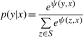
In the CRP model, we define the conditional probability, p(y|x), as follows:

(1)

where y is the vector of hidden LOH states, S is the set of all possible vectors of hidden LOH states and x is the vector of observations. The function ψ(y, x) is the sum of transition potentials and local evidences. In detail, the function is defined as follows:

(2)

where f_TP(y_t,y_t+1) is the transition potential function, f_LE(y_t, x) is the local evidence function and T is the number of SNPs. Next we will discuss the details of the two functions.

2.2 Transition potential

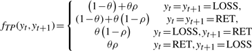
The transition potential function is selected so that the greater the distance between two neighboring SNPs, the greater the probability that the LOH status changes from one hidden state to the other. Here, we borrow the Haldane's map function (Lange, 2002) from the genetic recombination theory to model the relationship between transition probabilities and SNP distances. Mathematically, the transition function is defined as follows:

(3)

where θ=1 − e^−2d/β, and d is the distance between two SNPs, β is the transition decay parameter and ρ is the estimated LOH rate. The transition function is similar to that used in HMM methods for LOH inference (Affymetrix, 2007; Beroukhim et al., 2006). The function can be interpreted as the conditional probability of y_t+1 when the state of y_t is known, and θ is the probability that y_t+1 is not impacted by y_t. A larger β implies a slower transition from the current hidden state to a different hidden state and vice versa. In our experiments, β is empirically set as 10M bp as in Affymetrix (2007). The LOH rate ρ is estimated from the observations sequence.

2.3 Local evidence

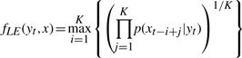
The local evidence for one hidden state y_t is the maximal support of the K consecutive neighboring observations. Mathematically, the local evidence is defined as follows:

(4)

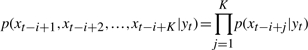
where p(x_j|y_t) is the emission probability that we observe x_j at locus j, while the hidden state in locus j is y_t. The detail of emission probability is defined below. The underlying assumptions are that the hidden state y_t holds on at least K consecutive loci nearby and the observations are independent. Therefore, the conditional probability that x_t−i+1, x_t−i+2,…,x_t−i+K are emitted from same hidden states as y_t , can be calculated as follows,

(5)

This can be regarded as the support (likelihood) that the hidden state in locus t is y_t when x_t−i+1, x_t−i+2,…,x_t−i+K are observed. The local evidence function looks for the best support for y_t from all observations around locus t in x (Fig. 1, where K=5).

The local evidence is one of the major differences between CRP and HMM. It can be considered as an adapted emission probability which smoothes the noise by integrating the information of neighboring SNPs and enforces that K consecutive probes have to have same state. Generally, the model with large K is expected robust to the errors, while smaller K is better for detecting small LOH regions in high quality data. In our experiments, K is set as 5 if not explicitly state. It should be noted that the CRP model with K=1 is not exactly equivalent to HMM, although they are very similar.

2.4 Emission probability

In the CRP model for the LOH inference problem, the hidden states are: loss of heterozygosity (LOSS) and retention (RET). There are nine observation states as defined in the Table 2, which are combinations of the genotypes in the normal and tumor samples.

Table 2.

Definition of observation states

Observation states		Tumor
		Homozygous	Heterozygous	NoCall
Normal	Homozygous	S1	S4	S5
	Heterozygous	S2	S3	S6
	NoCall	S7	S8	S9

The observations are obtained from the genotypes of tumor samples and normal reference samples of same patient. The emission probabilities p(x_t|y_t) used for the calculation of local evidences are given according to the quality of data and genotyping calls. In order to simplify the model, we assume that the genotyping errors in tumor samples and normal samples are independent and the heterozygous rate is constant over the whole genome. Additionly, this simple error model only considers the error that the homozygous SNP is called as heterozygous genotype or vice versa. The error that the homozygous SNP is called as another homozygous genotype is rare and omitted in the model.

Table 3 shows how the emission probabilities work out. Here, e₁ is the genotyping error rate in normal samples, e₂ is the genotyping error rate in tumor samples and h is the heterozygous rate of the normal samples. The heterozygous rate, h, is calculated from the genotype calls of normal samples. The genotyping error rate e₁ and e₂ is chosen empirically according to the output of genotyping software. Typically, we set e=0.02 which is also used in the LOH inference software of Affymetrix (2007). The value of e₂ is set as 2e₁ since the tumor samples often have a considerably higher genotyping error rate than normal samples.

Table 3.

Emission probability

Emission probability		Hidden states
		LOSS	RET
Observation states	S1	(1-e1)(1-e2)(1-h) +e1(1-e2)h	(1-e1)(1-e2)(1-h)+e1e2h
	S2	(1-e1)(1-e2)h +e1(1-e2)(1-h)	(1-e1)e2h+e1(1-e2)(1-h)
	S3	(1-e1)e2h+e1e2(1-h)	(1-e1)(1-e2)h+e1e2(1-h)
	S4	(1-e1)e2(1-h)+e1e2h	(1-e1)e2(1-h)+e1(1-e2)h
	S5	(1-e1)(1-h)+e1h	(1-e1)(1-h)+e1h
	S6	(1-e1)h+e1(1-h)	(1-e1)h+e1(1-h)
	S7	(1-e2)	(1-e2)(1-h)+e2h
	S8	e2	(1-e2)h+e2(1-h)
	S9	1	1

The simple probability model is illustrated in Figure 2. The probability of certain observation state (i.e. combination of genotypes in normal and tumor) is calculated from the conditional probabilities on the errors. For example, when the hidden state is LOSS, the emission probability of S1 (homozygous in both samples) is:

(6)

Since NoCall means the SNP is either homozygous or heterozygous, the probabilities of states with NoCall are the sum of the corresponding probabilities by replacing NoCall with homozygous or heterozygous. For example, when the hidden state is LOSS, the emission probability of S7 (NoCall in normal while homozygous in tumor) is:

(7)

The emission probability model is another major difference between CRP and existing HMM methods.

Fig. 2.

Emission probability model. The tables show the conditional probabilities of each combination of genotypes on the different error modes whose probabilities are shown above the arrows. Here, e₁ is the genotyping error rate in normal samples, e₂ is the genotyping error rate in tumor samples and h is the heterozygous rate of the normal samples.

2.5 LOH inference

Given observation sequence x, the hidden LOH status is inferred as:

(8)

which can be solved using Viterbi algorithm (Rabiner, 1989; Viterbi, 2006). In terms of computational complexity, the CRF algorithms have same asymptotic running times as HMM. Some well-developed software for CRF exists. In our experiments, a CRF toolbox for Matlab, CRFall,¹ written by Kevin Murphy, is used to solve the CRP model.

3 RESULTS

Several simulated and real tumor data are used to evaluate the developed CRP method. Both simulated and real data are from the Affymetrix Human Mapping 500K SNP arrays. The performance of CRP method is compared with to widely used HMM methods (Affymetrix, 2007; Beroukhim et al., 2006; Lin et al., 2004). We use two well-known implementations of HMM for LOH inference. One is the Affymetrix Genotyping Console (GTC) 2.0 software (Affymetrix, 2007) and the other is dChip (Lin et al., 2004). The genotype calls of GTC, which use BRLMM algorithm (Affymetrix, 2006), the official genotyping algorithm for the 500K SNP arrays, are used to generate the input of CRP method as well as HMM methods.

3.1 Data

The simulated data is based on the real 500K SNP arrays of HapMap samples provided in the Affymetrix website. The simulation is in the probe level and the simulated data are saved as Affymetrix's CEL files so that all software can process. Three samples are randomly selected as the normal reference samples: NA10851, NA12812 and NA18605. For each original normal sample and certain noise level, two simulated samples are generated: one for copy-loss LOH and the other for copy-neutral LOH. In each simulated sample, there are 50 LOH regions, including several whole chromosome LOH regions, several large LOH regions ranging from hundreds of SNPs to more than 10 000 of SNPs and several small LOH regions ranging from 20 SNPs to 100 SNPs. The mismatch probes are used as the background to calculate the simulated intensities of the corresponding perfect match probes in the LOH regions. The probes outside the LOH regions are unchanged. The noises are then simulated and added to all probes. The noise is assumed following a Gaussian distribution N(0, σ) where the SD of noise σ is proportional to the probe intensity y. The signal to noise ratio SNR=y/σ is changed from 5, 2 to 1.25 to simulate different noise levels. In total, 18 LOH samples are simulated from 3 normal samples, 6 (2 LOH types and 3 noise levels) for each normal sample. The simulated data can be downloaded from our website.²

There are two real datasets in the computational experiments. The first dataset is the nine tumor/normal pairs provided in the Affymetrix website, which are derived from human cancer cell lines. These include primary ductal carcinoma, non-small cell lung carcinoma and adenocarcinoma. The second is the myelodysplastic syndromes (MDS) samples in our laboratory. There are 20 patients in this dataset and three samples for each patient: one normal sample (lymphoid) and two tumor samples (blast and erythroid).

3.2 Results on simulated data

The call rates of the BRLMM algorithm for the simulated arrays range from 87.05% to 99.24% (Supplementary Table S1). The call rates decrease when the noise increases. The average call rates for the samples with SNR = 5, 2 and 1.25 are 98.23%, 93.62% and 89.16% respectively. When other conditions are the same, the call rates for copy-less LOH samples are smaller than the copy-neutral LOH samples.

The results of CRP method are compared with that of HMM methods implemented in GTC 2.0 and dChip. The results of the SNPs that are heterozygous in the normal sample are shown in Table 4. Two HMM implements show different bias: GTC tends to minimize the false positive rate (FPR), while dChip prioritizes the high true positive rate (TRP). This observation is confirmed by the receiver operating characteristic (ROC) graphs in Figure 3. Compared to GTC, CRP obtains significantly higher TPR while maintaining the same low FPR. Compared to dChip, CRP had much lower FPR and slightly better TPR. The P-values of the differences between the ROC curves of CRP and other methods are calculated by using the approach described by DeLong et al. (1988). All P-values are smaller than 10⁻²⁰⁰ (Supplementary Table S2) which means the differences between CRP and other methods are statistically significant.

Table 4.

Results of simulated data for informative SNPs

SNR	Samples	LOH type	CRP		HMM(GTC)		HMM (dChip)
			TPR	FPR	TPR	FPR	TPR	FPR
5.00	NA10851	CN = 1	0.9984	0.0003	0.9736	0.0003	0.9907	0.0103
		CN = 2	0.9982	0.0003	0.9842	0.0003	0.9906	0.0106
	NA12812	CN = 1	0.9984	0.0004	0.9645	0.0003	0.9905	0.0108
		CN = 2	0.9982	0.0002	0.9801	0.0003	0.9905	0.0103
	NA18605	CN = 1	0.9979	0.0004	0.9728	0.0002	0.9904	0.0118
		CN = 2	0.9980	0.0004	0.9852	0.0002	0.9904	0.0120
2.00	NA10851	CN = 1	0.9984	0.0031	0.9353	0.0085	0.9922	0.0183
		CN = 2	0.9987	0.0048	0.9724	0.0076	0.9914	0.0184
	NA12812	CN = 1	0.9991	0.0055	0.9227	0.0159	0.9917	0.0268
		CN = 2	0.9990	0.0041	0.9622	0.0109	0.9914	0.0214
	NA18605	CN = 1	0.9991	0.0088	0.9364	0.0110	0.9926	0.0231
		CN = 2	0.9988	0.0050	0.9720	0.0105	0.9918	0.0212
1.25	NA10851	CN = 1	0.9991	0.1798	0.8878	0.2002	0.9954	0.2531
		CN = 2	0.9996	0.1322	0.9387	0.1672	0.9951	0.2096
	NA12812	CN = 1	0.9989	0.2592	0.8731	0.2875	0.9962	0.3700
		CN = 2	0.9999	0.2291	0.9251	0.2453	0.9966	0.3149
	NA18605	CN = 1	0.9987	0.1876	0.8860	0.2211	0.9959	0.2875
		CN = 2	0.9991	0.1671	0.9381	0.1936	0.9954	0.2536

Fig. 3.

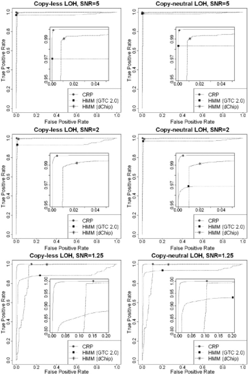
ROC curves of the CRP and HMM methods for informative SNPs. Left are copy-less LOH simulations, while right are copy-neutral LOH (UPD) cases. The highlighted points are default outputs of algorithms.

As shown in Table 4 and Figure 3, the TPR of HMM methods for the copy-less samples are significantly lower than that of copy-neutral cases. We believe that it is due to the genotyping algorithm which produces more errors in the copy-less regions than the copy-neutral regions. In other words, HMM method in GTC is not robust when the genotyping error rate is relatively large in the copy-less LOH regions.

One of the important goals of the LOH inference is to predict the LOH status of non-informative SNPs. The inference capability of the CRP method on the non-informative SNPs is illustrated in Table 5. Since GTC only infer the LOH status for the heterozygous SNPs of the normal sample, the results are only compared between CRP and dChip. The TPR and FPR of CRP method are very close to informative SNPs. The high TRP and low FPR show that CRP method can precisely reveal the LOH status for non-informative SNPs as well as informative SNPs. Compared with dChip, the TPR of CRP are slightly better, but the FPR are 10-fold smaller than dChip in low-noise cases (SNR=5) and 2-fold smaller in high-noise cases (SNR = 1.25).

Table 5.

Results of simulated data for non-informative SNPs

SNR	Samples	LOH type	CRP		HMM (dChip)
			TPR	FPR	TPR	FPR
5.00	NA10851	CN = 1	0.9943	0.0013	0.9925	0.0256
		CN = 2	0.9939	0.0014	0.9924	0.0230
	NA12812	CN = 1	0.9943	0.0013	0.9920	0.0248
		CN = 2	0.9940	0.0003	0.9921	0.0228
	NA18605	CN = 1	0.9925	0.0008	0.9917	0.0258
		CN = 2	0.9925	0.0008	0.9916	0.0249
2.00	NA10851	CN = 1	0.9906	0.0026	0.9936	0.0555
		CN = 2	0.9950	0.0041	0.9932	0.0506
	NA12812	CN = 1	0.9955	0.0053	0.9932	0.0573
		CN = 2	0.9952	0.0035	0.9930	0.0543
	NA18605	CN = 1	0.9956	0.0070	0.9935	0.0515
		CN = 2	0.9939	0.0043	0.9929	0.0509
1.25	NA10851	CN = 1	0.9939	0.1469	0.9959	0.2790
		CN = 2	0.9967	0.1054	0.9958	0.2414
	NA12812	CN = 1	0.9963	0.2312	0.9967	0.4088
		CN = 2	0.9991	0.1997	0.9975	0.3614
	NA18605	CN = 1	0.9940	0.1662	0.9967	0.3145
		CN = 2	0.9960	0.1431	0.9953	0.2707

The CRP method reports more compact LOH segments, i.e. less over-segmentation than other methods (Supplementary Table S3). Extensive experiments with a range of parameters show that the CRP method is robust to the changes of parameters (Supplementary Figs S1–S3).

3.3 Results on Affymetrix's tumor data

The Affymetrix's data is obtained from high-quality control experiments. The call rates of BRLMM algorithm range from 93.32% to 99.21%, and the average call rate is 97.41%. The LOH inference results of three methods are very similar except for several small regions. Figure 4 shows an example of the whole-genome results of the paired tumor/normal samples CCL-256D/CCL-256.1D.

Fig. 4.

The results of CRP and HMM methods, on Affymetrix's tumor/normal sample pair CCL-256D/CCL-256.1D. The horizontal axis is the ordered SNPs in whole genome, and the vertical bar indicates the LOH.

3.4 Results on MDS data

The qualities of SNP arrays for MDS samples are varied and not high as that of Affymetrix's data. The call rates of BRLMM algorithm range from 85.4% to 98.41%. The average call rate is 94.89%. Therefore, the LOH inference algorithm tends to make more false predictions. As in the Affymetrix's tumor data, the CRP method and HMM methods produce similar results in large LOH regions.

The result of one patient MDS-8 is shown in Figure 5. All methods predict that the chromosome 7 is LOH in blast and erythroid samples, which is confirmed by CN analysis. But the inferences of small LOH regions are different. Since the blast and erythroid samples are from the same individual, we expect to observe the same (or similar) LOH patterns in the two samples. Overall, the results of CRP method are more consistent between the two tumor samples. The consistency statistics between the results of two tumor samples by several methods are drawn in Figure 6. More than 80% of the inferred LOH SNPs in two samples by CRP are overlapped. However, for HMM, there are only 65% and 76% overlaps, respectively. Another result of the patient MDS-6 is shown in Figures 7 and 8. Again, the CRP method produces more common inferred LOH SNPs between two tumor samples in terms of both percentage and number. The results of other patients are similar. Since the tumor may gain or lose LOH regions as it progresses, the consistency between different fractions may not be a good measurement for the accuracy of LOH inference methods. Nevertheless, the common LOH regions of different samples may have a higher value for the downstream analysis such as identification of disease SNPs and genes.

Fig. 5.

The results of CRP and HMM methods, on blast and erythroid samples of patient MDS-8. The horizontal axis is the ordered SNPs in whole genome, and the vertical bar indicates the LOH. From top to bottom: CRP result of blast, HMM (GTC) result of blast, HMM (dChip) result of blast, CRP result of erythroid, HMM (GTC) result of erythroid and HMM (dChip) result of erythroid.

Fig. 6.

Numbers and percentages of inferred LOH SNPs in two tumor samples from same patient MDS-8.

Fig. 7.

The results of CRP and HMM methods, on blast and erythroid samples of patient MDS-6. The horizontal axis is the ordered SNPs in whole genome, and the vertical bar indicates the LOH. From top to bottom: CRP result of blast, HMM (GTC) result of blast, HMM (dChip) result of blast, CRP result of erythroid, HMM (GTC) result of erythroid and HMM (dChip) result of erythroid.

Fig. 8.

Numbers and percentages of inferred LOH SNPs in two tumor samples from same patient MDS-6.

4 CONCLUSION

In this article, a novel LOH inference and segmentation algorithm based on CRP model is presented. The algorithm explores more contextual information from neighboring SNPs by considering the genotyping error rate, the heterozygosity rate and the distances between SNPs. There are two major differences between the CRP method and the existing HMM methods. One is the local evidence exploiting the information of neighboring SNPs. The other is the new emission probability model. For informative SNPs, the CRP method can recover the mistakes due to genotyping error, as shown in the experiments with simulated data. The CRP method can also reliably infer the LOH status for non-informative SNPs. The new method infers the LOH status for those SNPs with no genotype calls as well, which is not considered in the existing literature. The experiments of simulated and real data show that the CRP method is effective and reliable for LOH inference and segmentation.

The proposed CRP method works well for the paired tumor/normal samples from the same individual. Although the CRP model can be adapted to the unpaired case, the LOH inference for the unpaired tumor samples is a different problem. Due to the lack of normal reference, the FPR will be very high if the LOH inference is only based on the genotype calls of tumor samples (Beroukhim et al., 2006). Therefore, the extension of CRP method to analyze unpaired tumor samples should consider additional information such as SNP-specific heterozygosity rates, haplotype structures and recombination rates. This is one of our ongoing studies. Another future research direction is to integrate the CN variation analysis into the CRP model. By directly modeling the hybridization intensity, the LOH inference method may be more powerful and less dependent on the accuracy of genotyping algorithm.

References

- Affymetrix. BRLMM: an Improved Genotype Calling Method for the GeneChip Human Mapping 500K Array Set. Whitepaper, Affymetrix; 2006. [Google Scholar]
- Affymetrix. CNAT 4.0: Copy Number and Loss of Heterozygosity Estimation Algorithms for the GeneChip Human Mapping 10/50/100/250/500K Array Set. Whitepaper, Affymetrix; 2007. [Google Scholar]
- Albertson DG, Pinkel D. Genomic microarrays in human genetic disease and cancer. Hum. Mol. Genet. 2003;12:R145–R152. doi: 10.1093/hmg/ddg261. [DOI] [PubMed] [Google Scholar]
- Beroukhim R, et al. Inferring loss-of-heterozygosity from unpaired tumors using high-density oligonucleotide SNP arrays. PLoS Comput. Biol. 2006;2:e41. doi: 10.1371/journal.pcbi.0020041. [DOI] [PMC free article] [PubMed] [Google Scholar]
- DeLong ER, et al. Comparing the areas under two or more correlated receiver operating characteristic curves: a nonparametric approach. Biometrics. 1988;44:837–845. [PubMed] [Google Scholar]
- Eeles RA, et al. Multiple newly identified loci associated with prostate cancer susceptibility. Nat. Genet. 2008;40:316–321. doi: 10.1038/ng.90. [DOI] [PubMed] [Google Scholar]
- Gudmundsson J, et al. Common sequence variants on 2p15 and Xp11.22 confer susceptibility to prostate cancer. Nat. Genet. 2008;40:281–283. doi: 10.1038/ng.89. [DOI] [PMC free article] [PubMed] [Google Scholar]
- Huang J, et al. Whole genome DNA copy number changes identified by high density oligonucleotide arrays. Hum. Genomics. 2004;1:287–299. doi: 10.1186/1479-7364-1-4-287. [DOI] [PMC free article] [PubMed] [Google Scholar]
- Knudson AG. Two genetic hits (more or less) to cancer. Nat. Rev. Cancer. 2001;1:157–162. doi: 10.1038/35101031. [DOI] [PubMed] [Google Scholar]
- Lafferty JD, et al. Proceedings of the Eighteenth International Conference on Machine Learning. San Francisco, CA, USA: 2001. Conditional random fields: probabilistic models for segmenting and labeling sequence data. [Google Scholar]
- Lafferty JD, et al. Proceedings of the Twenty-First International Conference on Machine Learning. Banff, Alberta, Canada: 2004. Kernel conditional random fields: representation and clique selection. [Google Scholar]
- Lange K. Mathematical and Statistical Methods for Genetic Analysis. New York: Springer-Verlag; 2002. [Google Scholar]
- Lin M, et al. dChipSNP: significance curve and clustering of SNP-array-based loss-of-heterozygosity data. Bioinformatics. 2004;20:1233–1240. doi: 10.1093/bioinformatics/bth069. [DOI] [PubMed] [Google Scholar]
- Lindblad-Toh K, et al. Loss-of-heterozygosity analysis of small-cell lung carcinomas using single-nucleotide polymorphism arrays. Nat. Biotechnol. 2000;18:1001–1005. doi: 10.1038/79269. [DOI] [PubMed] [Google Scholar]
- McEvoy C.RE, et al. Evidence for whole chromosome 6 loss and duplication of the remaining chromosome in acute lymphoblastic leukemia. Genes Chromosomes Cancer. 2003;37:321–325. doi: 10.1002/gcc.10214. [DOI] [PubMed] [Google Scholar]
- Pinto D, et al. Proceedings of the 26th Annual International ACM SIGIR Conference on Research and Development in Informaion Retrieval. Toronto, Canada: 2003. Table extraction using conditional random fields. [Google Scholar]
- Rabiner LR. A tutorial on hidden Markov-models and selected applications in speech recognition. Proc. of the IEEE. 1989;77:257–286. [Google Scholar]
- Sha F, Pereira F. Proceedings of the 2003 Conference of the North American Chapter of the Association for Computational Linguistics on Human Language Technology. Edmonton, Canada: 2003. Shallow parsing with conditional random fields. [Google Scholar]
- Viterbi AJ. A personal history of the Viterbi algorithm. IEEE Signal Proc. Mag. 2006;23:120–142. [Google Scholar]
Associated Data
This section collects any data citations, data availability statements, or supplementary materials included in this article.