Modeling the Effects of Vaccination and Treatment on Pandemic Influenza

Abstract

In this paper, we demonstrate the uses of some simple mathematical models for the study of disease dynamics in a pandemic situation with a focus on influenza. These models are employed to evaluate the effectiveness of various control programs via vaccination and antiviral treatment. We use susceptible-, infectious-, recovered-type epidemic models consisting of ordinary differential equations. These models allow us to derive threshold conditions that can be used to assess the effectiveness of vaccine and drug use and to determine disease outcomes. Simulations are helpful for examining the potential consequences of control options under different scenarios. Particularly, results from models with constant parameters and models with time-dependent parameter functions are compared, demonstrating the significant differences in model outcomes. Results suggest that the effectiveness of vaccination and drug treatment can be very sensitive to factors including the time of introduction of the pathogen into the population, the beginning time of control programs, and the levels of control measures. More importantly, in some cases, the benefits of vaccination and antiviral use might be significantly compromised if these control programs are not designed appropriately. Mathematical models can be very useful for understanding the effects of various factors on the spread and control of infectious diseases. Particularly, the models can help identify potential adverse effects of vaccination and drug treatment in the case of pandemic influenza.

INTRODUCTION

Mathematical models may be helpful for studying the transmission and control of infectious diseases. This area of study has been highlighted recently due to the advent of a new strain of pandemic influenza, worries about the possible reintroduction of smallpox and the emergence of new pathogens such as the SARS coronavirus. The mathematical theory pioneered by Ross, MacDonald, Kermack, McKendrick, and others has played a major role in the prevention and control of infectious diseases (see also (1)). More recently, researchers have used mathematical models to better understand influenza dynamics and to investigate how to effectively control influenza via various strategies including antiviral treatment and vaccination (see, for example, (2–6)).

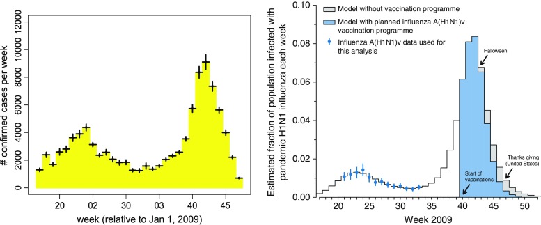
We have previously used a simple mathematical model to forecast the course of the 2009 influenza A (H1N1) pandemic in the USA (see (7)). In that study, we fit the model to the Centers for Disease Control and Prevention (CDC) influenza data collected during early months of the year, optimizing the model parameters associated with the time-dependent transmission, and the time at which the initial case was introduced. The optimized model was then used to forecast the timing of the autumn wave of infection (see (8)). The most striking feature of the model is that it accurately predicted the peak time of the pandemic. According to the CDC 2009 H1N1 surveillance reports (9), the peak of the fall wave was reached at the end of October (which is between weeks 42 and 43, see the left-hand plot in Fig. 1), which is consistent with our model result (see the right-hand plot in Fig. 1).

Fig. 1.

Comparison of predictions with observations. The left figure illustrates the CDC 2009 H1N1 confirmed case count data, as obtained from CDC weekly surveillance data in reference CDC (2009) (the error bars represent variations calculated by the authors to account for US regional variability in the timing of the pandemic). The right figure shows predictions of Towers and Feng (7). The model used in that analysis is of the form (2.1), and the parameter values were β ₀ = 0.52, ε = 0.35, γ = 1/3, and t ₀ = 55

In this paper, we present some simple mathematical models that can be used to study the impact of vaccination and antiviral drug treatment on the spread and control of infectious diseases such as influenza. We focus on models consisting of differential equations that are of the susceptible, infectious, recovered (SIR) type with time-dependent functions representing vaccination and treatment policies. A seasonally forced disease transmission rate is also included to reflect the fact that the transmission rate may be higher in some seasons than others.

For the case of a constant transmission rate, the basic reproduction number and the control reproduction number have been shown to determine the prevalence of infection and the severity of disease outbreaks (1). The formula is a function of the levels of vaccination and antiviral use, and reveals that these control measures are always beneficial in mitigating the disease outbreak (see “The Case of Constant Parameters” section).

However, for the case of periodic transmission rate, our simulation results show that whether and how much these control measures are helpful depends on many factors, including the timing and intensity of the programs, as well as the time of introduction of infections. Particularly, our results suggest that in some cases, an increased level of vaccination or antiviral use may actually lead to higher epidemic peaks and/or larger final epidemic sizes (see results presented in “The Case of Time-Dependent Parameters” section).

This paper is organized as follows; in the “Model Descriptions” section, we introduce the SIR models used for our analysis and simulations. The “Results from Model Analysis and Simulations” section describes the main results and their implications for public health. Comparisons of effects of various vaccination and treatment programs on disease control are also presented in the “Results from Model Analysis and Simulations” section. The “Discussion” section includes a summary and further discussion of the results.

MODEL DESCRIPTIONS

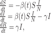
One of the simplest epidemiological models is the SIR epidemic model, in which the total population is divided into three epidemiological classes: susceptible (S), infected (and infectious, I), and recovered (R) individuals. Let S = S(t), I = I(t), and R = R(t) denote the numbers of individuals at time t in the corresponding classes, and let N = S + I + R denote the total population size. A deterministic epidemic model using ordinary differential equations consists of the following equations

2.1

with initial conditions

2.2

where, I₀ > 0 is a constant. In the initial conditions (2.2), t₀ > 0 denotes the time of introduction of the infection into the population, and it will be shown later that t₀ is a critical parameter of the model when the transmission rate β(t) is a periodic function due to seasonality. Note that t = 0 corresponds to the first day of a calendar year and t₀ is the number of days from t = 0. The model (2.1) ignores vital dynamics (births and deaths), which is a reasonable assumption when modeling a pandemic.

If vaccines are available before the epidemic starts, a certain level of population immunity can be achieved via vaccination. Let p₀ denote the level of population immunity at time t₀. Then the disease dynamics can be modeled by the equations in (2.1) with modified initial conditions:

2.3

We do not include vaccinated individuals in the R class because the value of R(t) at the end of the disease outbreak will be used to measure the final epidemic size. In system (2.1), a standard incidence form is used for new infections and the function β(t) represents the rate at which a susceptible individual becomes infected when contacting an infectious individual. The duration of infection is assumed to follow an exponential distribution with the mean period 1/γ; and thus, γ is the per capita recovery rate.

In most deterministic epidemic models, β(t) = β₀ is assumed to be constant. However, for many diseases, seasonal variation in the transmission rate can be important. Any periodic function can be expressed as an infinite sum of sines and cosines. In this analysis, we express the periodic transmission rate as the first-order harmonic with a 1-year period:

2.4

where, β₀ is a constant representing a background transmission rate and ε is a constant related to the magnitude of the seasonal fluctuation. The function β(t) given in (2.4) has its maximum at the beginning of a calendar year. When the transmission rate is expressed in this form, the time of introduction of the pathogen to the population t₀ is a crucial parameter of the seasonal model because the final size and shape of the epidemic curve (including how many peaks the epidemic exhibits within one calendar year) can depend quite strongly on this parameter (whereas for models with constant β, the final size and shape are independent of t₀). Further, the shape of the epidemic curve also strongly depends on the initial fraction of susceptibles in the population at t₀ when β(t) is periodic.

All the variables and parameters as well as their definitions are listed in Table I.

Table I.

Definition of Symbols and Parameter Values Used in Simulations

Symbols	Definition	Value (range)
S(t)	Number of susceptible individuals at time t
I(t)	Number of infectious individuals at time t
I u(t) (I tr(t))	Number of untreated (treated) infectious at time t
R(t)	Number of recovered individuals at time t
t 0	Time of introduction of the pathogen to the population Varied	Varied
β 0	Background transmission rate
ε	Related to the oscillation amplitude	0.35
γ u	Recovery rate of untreated individuals	1/γ u = 3 (days)
γ tr	Recovery rate of treated individuals	1/γ tr = 2 (days)
	Proportion of susceptibles vaccinated	[0, 1]
η	Efficacy of vaccine	[0, 1]
	Proportion of susceptibles successfully vaccinated	[0, 1]
f 0	Proportion of infections treated	[0, 1]
t v	Beginning times of vaccination	Varied
σ	Reduction in transmission due to treatment	0.5

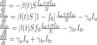
The model (2.1) can be extended to include both vaccination and antiviral drug treatment. Let f₀ denote the fraction of infected individuals who will receive treatment at time t; I_u and I_tr denote the numbers of untreated and treated infected individuals, respectively; and let the infectious period for an untreated individual is 1/γ_u. Assume that treatment reduces infectiousness by a factor σ and reduces the infectious period to 1/γ_tr < 1/γ_u. Following the approach of Lipsitch et al. (6) to model drug treatment, we can extend the model (2.1) as

2.5

with initial conditions

2.6

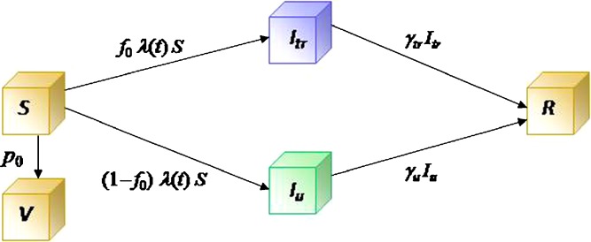
where I_u0 is a positive constant representing the initial number of infected people. A transition diagram between the epidemiological classes is shown in Fig. 2.

Fig. 2.

A transition diagram between the epidemiological classes for model (2.5). The compartments are S (susceptible), I _u (infected untreated), I _tr (infected treated), R (recovered). The V class includes individuals who are immune to further infection due to vaccination. The λ function in the transmission term is defined by , where β(t) denotes the transmission rate and σ ≤ 1 represents a reduction in infectiousness due to treatment. The constants p ₀ and f ₀ are the fractions of vaccinated susceptible and treated infectious individuals respectively. γ _u and γ _tr are the rates of recovery for the untreated and treated individuals, respectively

Where there is a delay in the supply of vaccines, we could still use equations in (2.5) with modifications. For example, let t_v > t₀ denote the time at which the vaccination program starts and assume that a fraction p₀ of the remaining susceptibles will be vaccinated at the time t_v. We can first use equations in (2.5) and the initial conditions (2.6) with p₀ = 0 for simulations in the interval . For the time after t_v, we can continue to use the equations in (2.5), but with new initial conditions (1−p₀)S(t_v), I(t_v), and R(t_v).

In the next section, we will present some analysis and simulations of the models discussed above and then use the results to examine the effects of vaccination and treatment on disease mitigation and control.

RESULTS FROM MODEL ANALYSIS AND SIMULATIONS

In this section, we study models (2.1) and (2.5) and present results under two scenarios: case 1 is for constant rates and case 2 is for periodic transmission rate and time-dependent vaccination and treatment.

The Case of Constant Parameters

In epidemiological models, one of the most important quantities is the basic reproduction number denoted by . The definition of for models with constant parameters is the average number of secondary infections produced by one infected individual during his/her entire period of infection in a wholly susceptible population. This number determines whether there will be an outbreak of the disease when an infectious person is introduced into the population and how severe the outbreak will be in the absence of any programs of disease control and prevention.

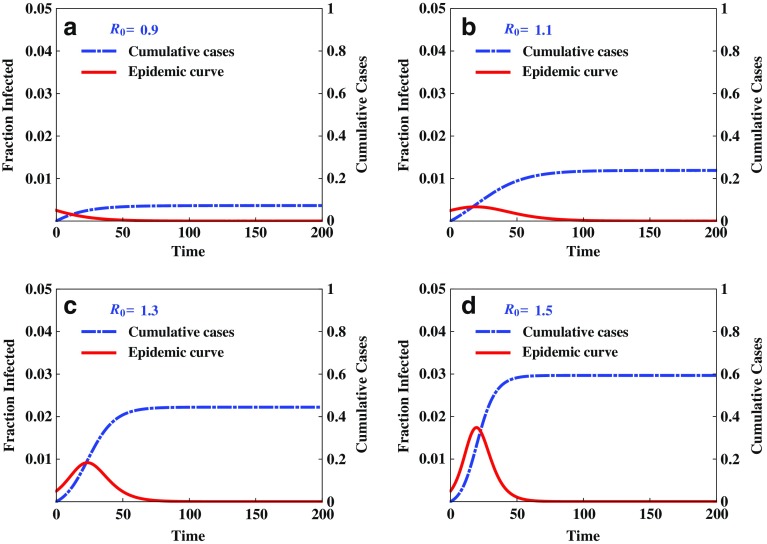
Figure 3 illustrates the disease outcomes of system (2.1) with the initial condition (2.2) and constant transmission rate β₀. It demonstrates that the threshold condition determines whether there will be an outbreak or not . It also shows clearly that the severity of an epidemic depends on the magnitude of the reproduction number .

Fig. 3.

Illustration of disease outcomes from system (2.1) with initial conditions (2.2) and constant β ₀. The epidemic curve and cumulative cases are plotted for various values of , showing clearly the dependence of the severity of an epidemic on the magnitude of . That is, there will be no outbreak if (see a), whereas if then an outbreak will occur with the final epidemic size increases with (see b–d)

Besides the kind of deterministic outcomes presented in Fig. 3, the modeling structure shown in (2.1) can also be used to simulate the situations in which the disease events (e.g., infection and recovery) may occur randomly (while being governed by the event rates determined by the equations in (2.1)). By incorporating the randomness of disease transmission process, the models will be capable of providing helpful information about how likely a certain disease outcome will be expected under a given condition. One of the approaches for stochastic simulations is the event/time approach (10). Consider the model (2.1) with constant transmission rate β. There are only two possible events at time t_i (i = 0, 1, 2, ···); a new infection which occurs at the rate r₁(t_i) = βS(t_i)I(t_i)/N and a recovery which occurs at the rate r₂(t_i) = γI(t_i). Let denote the total event rate at time t_i. Then the “time to next event”, T_i, can be determined by

where, Y₁ is a random number generated from the exponential distribution with parameter r_T(t_i). To determine which of the two events occurs at time , we use another random number, Y₂, generated from a uniform distribution on [0, 1]. For example, if

then the first event (infection) occurs, in which case

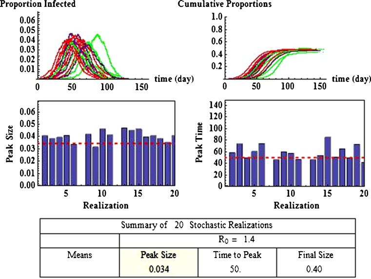
Some of these results using this approach are illustrated in Fig. 4. It shows 20 realizations (repeated runs with the same set of parameters), which are represented by different colors in the top two figures. For demonstration purposes, the parameter values used are β = 0.45 and γ = 1/3, (for which ) and I₀ = 5 with N = 20,000. Effects of model parameters (e.g., ) on the disease outcomes can be examined by computing the statistics generated from the stochastic simulations. For example, among the 20 realizations, each of which showing different peak and final sizes and the time at the peak, the means are: epidemic peak = 34% of the population, peak time = 50 days, and the final size = 40% of the population. The histograms show the variations of the 20 epidemic peak sizes and peak times around the respective means.

Fig. 4.

Stochastic simulations of model (2.1) with initial conditions (2.2). It shows 20 repeated runs with same parameter values and the curves with different colors in the top two figures represent the paths in the 20 different runs. The top-left plot shows all 20 epidemic trajectories and the top-right plot shows all 20 curves of cumulative infections. The histograms illustrate the variations of peak sizes and the peak times relative to the respective means (dashed line). A summary of the mean values of the 20 realizations is provided in the table on the bottom, showing that the mean value of the epidemic sizes is 34% of the population, the mean of peak times is 50 days, and the mean final sizes is 40% of the population

We now consider the model (2.5). When control programs are implemented, the corresponding reproduction number is commonly called the control reproduction number and denoted by (c for control). One objective of control programs is to reduce to below one, and the best strategy is usually the one that reduces the most and the fastest for given resources. In the case when β(t) = β₀ is a constant for all t ≥ t₀, and when vaccines are available at t₀, the reproduction numbers for the model (2.5) are given by

3.1

It is clear that in the absence of vaccination and treatment, i.e., when p₀ = f₀ = 0. For p₀ > 0 and/or f₀ > 0, since σ ≤ 1 and γ_tr ≥ γ_u,

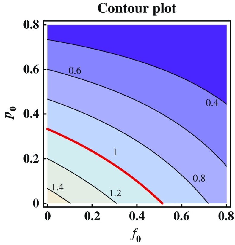
In fact, is a decreasing function of p₀ and f₀ as shown in Fig. 5. An explicit formula for such as the one given in (3.1) can be very helpful for designing control programs. For example, if the objective of a control measure is to reduce to below a presubscribed value , then we can use this formula to determine the combined efforts of vaccination and treatment needed to achieve the goal . The levels of vaccination p₀ and treatment f₀ which will lead to are identified in Fig. 5. Several curves corresponding to different values are labeled with the thicker curve corresponding to . We observe that all points (p₀, f₀) above the curve will lead to , in which case the disease cannot take off.

Fig. 5.

Contour plot showing the dependence of on p ₀ and f ₀. Several curves corresponding to different values are labeled with the thicker curve corresponding to . It shows also that for all points (p ₀ , f ₀) above the curve in which case the disease cannot take off

Note that the parameter p₀ in the function denotes the proportion of successfully vaccinated people. If the efficacy of vaccine is not 100%, then where η and denote respectively the efficacy of vaccine and the proportion of vaccinated population. In this case, the formula for can also be considered as a function of η, and f₀ given by

This formula allows us to evaluate the effect of improved vaccines. For example, in the absence of treatment (i.e., f₀ = 0) the control reproduction number is a function of η and only. This relation is plotted in Fig. 6. The curve corresponding to the threshold condition, , is identified in the contour plot. For a given proportion , we can use this curve to determine the minimum efficacy η_min such that for all η > η_min. The contour curves can also help us identify optimal combinations of η and to achieve certain objectives. For example, suppose that the costs of vaccination and vaccine improvement are known and the total cost to successfully vaccinate a proportion of the susceptibles can be determined, denoted by. Then for a presubscribed value , we can determine the optimal levels η_opt and that minimizes the total cost under the constraint

Fig. 6.

Contour plot showing the dependence of Rc on η and with f ₀ = 0. This figure is similar to Fig. 5 but with p ₀ and f ₀ replaced by η and . The thicker curve is the curves along which . It shows that for all points above the curve, in which case the disease cannot take off.

The Case of Time-Dependent Parameters

When model parameters vary with time, analytical results such as the threshold conditions described in (3.1) will be very difficult to obtain. Most results are based on numerical simulations. In this section, we present examples in which the transmission rate β(t) has the form as in (2.4), with possible delayed vaccination uses, i.e., t_v ≥ t₀. These scenarios are based on the consideration that vaccines and antiviral drugs may not be available at the beginning of an epidemic. We will again focus on three important measures when assessing the effect of a control program: (a) peak size of the epidemic curve (the maximum number of infections during the course of a pandemic), (b) peak time (the time at which the peak occurs), and (c) final size (the total number of infections at the end of a pandemic). Main objectives of effective control strategies should include lowering the peak size to keep demand for facilities below available supply, lowering the final size to reduce morbidity, and delaying the peak to provide more time for response.

Unlike in the case of constant parameters, where vaccination and treatment will always help reduce morbidity (see Fig. 5), the case of periodic transmission rate β(t) may generate non-intuitive results. That is, the model can exhibit outcomes in which an increased use of vaccination or antiviral drugs will lead to a higher morbidity. To demonstrate this, we first consider the simpler case in which the model (2.1) with the initial conditions given in (2.3) is used. This represents the case when vaccination starts immediately when new infections are introduced into the population. One such example is presented in Fig. 7.

Fig. 7.

Plots of epidemic curves and cumulative infections for different values of t ₀. These plots show the dramatic effect that the start time of an epidemic (t ₀) can have on its progression in a periodic environment given by the SIR model (2.1) with initial conditions (2.2), where I ₀ = 1 and N = 10⁷. From the plots in a and c we observe that when t ₀ = 30, vaccination reduced both the peak size and the peak time although there is not much delay in the peak time. However, plots in b and d show that, although the size of the first epidemic peak is reduced, a second (and higher) peak is also generated. More significantly, the final epidemic size is increased, showing the sensitivity of the behaviors of the epidemic to t ₀

In Fig. 7, both the epidemic curve and curve representing the cumulative infections are plotted. For the transmission function β(t), the parameter values used are those of an H1N1-like disease with β₀ = 0.5 and ε = 0.35. We assume 1/γ = 3 days. These values are also used in other figures except when specified differently. The figure shows two sets of simulations corresponding to two different times (t₀) of initial introduction of pathogens. One case is for t₀ = 30 and the other is for t₀ = 40, and for demonstration purposes the vaccination level is chosen to be p₀ = 0.1.

Some interesting observations can be made from Fig. 7. We can first compare the outcomes between the model without vaccination (the solid curves) and the model with vaccination (the dashed curves). It demonstrates the dependence of the model outcomes on the time of introduction (t₀) of initial infections. Particularly, we observe that although the peak and final sizes are both decreased for the case of t₀ = 30, the case of t₀ = 40 differs significantly. Although the first wave is reduced, the second wave is also generated. Moreover, the final epidemic size is even higher than that without vaccination, demonstrating a scenario in which the use of vaccine may have a detrimental consequence.

In the next example, we use the model (2.1) with initial conditions given in (2.3) to examine the interplay between t₀, t_v, and p₀, as well as their influence on the effect of vaccination programs. In Fig. 8, we consider two t₀ values; t₀ = 30 in panel a and t₀ = 40 in panel b. In each of these panels, model outcomes corresponding to different levels of vaccination (p₀) are compared. When t₀ = 30, panel a shows that the effect of vaccination use on the peak and final sizes are not monotone. That is, the peak and/or final sizes may either decrease or increase with p₀. When t₀ is increased from 30 to 40, panel b shows that, although the final sizes decreases monotonically when p₀ is increased from 0.1 to 0.25, the final epidemic size for the case of p₀ = 0.1 is actually higher than that without vaccination use.

Fig. 8.

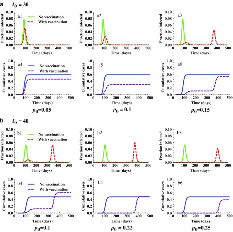
Comparison of epidemic severity for different values of t ₀ and p ₀ with f ₀ = 0. It shows the joint influence of t ₀ and p ₀ on the effect of vaccination programs. The initial conditions used are the same as in Fig. 7. Plots in a show that the peak and final sizes are decreased when p ₀ is increased from 0.05 (see a1 and a4) to 0.1 (see a2 and a5). However, when p ₀ continues to increase from 0.1 to 0.15, one epidemic peak becomes two with the second peak higher than the first (see a3 and a6), and the final epidemic size is larger than the case of p ₀ = 0.1. This differs from the case of t ₀ = 40 shown in b. In this case, for the lower p ₀ value (p ₀ = 0.1) two peaks occurred and the final size is higher than that without vaccination use (compare b1 and b4). However, when p ₀ exceeds 0.22 the peak and final sizes will not be higher than those without vaccination use. Both peak and final sizes will continue to decrease when p ₀ increases (see b2–b3 and b5–b6)

We now examine the simulation results from the model (2.5), which includes also drug treatment, with possible delays in vaccination use. Simulations illustrated in Figs. 9 and 10 show how the peak and final epidemic sizes may vary with p₀ (the levels of vaccination), f₀ (drug treatment), and t_v (the starting time of vaccination). Figure 9 plots the epidemic curves and final epidemic sizes for the case of t₀ = 35 under various levels of vaccination (p₀) without treatment (f₀ = 0). Notice that for t₀ = 35, there is only a single peak in the epidemic curve in the absence of vaccination and treatment (see a). Simulation results for two different values t_v are demonstrated in the middle panel (t_v = 60) and the bottom panel (t_v = 100). In each panel, outcomes for three p₀ values are compared. A dramatic difference is that for the case of t_v = 60 the peak and final epidemic sizes exceed those without vaccination use, whereas for the case of t_v = 100 the peak and final size decrease monotonically with increasing p₀. We need to point out that although this set of simulations suggest that an earlier start of vaccination use is not beneficial (due to an increased peak and final sizes), this may not be the cases for other values of t₀ (simulations not shown here). That is, whether and how much vaccination can help to reduce the severity of epidemics depends jointly on t_v and t₀.

Fig. 9.

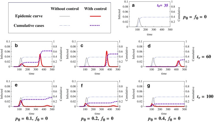
Comparison of epidemic severity for different values of t _v and p ₀ with f ₀ = 0. These plots of epidemic curves and final epidemic sizes are for the case of t ₀ = 35 with two values of t _v (the time when vaccination begins) under three different levels of vaccination (p ₀) and no treatment (f ₀ = 0). The model used is (2.5) with initial conditions (2.6), where I _u0 = 1 and N = 305 million. Notice that there is only a single peak in the epidemic curve in the absence of control (see a); a is for the case of no vaccination (p ₀ = 0). Two different starting times of vaccination (t _v) are examined: b–d are for t _v = 60, whereas e–g are for t _v = 100. For each t _v value, three levels of vaccination use are considered: p ₀ = 0.1 (b and e), p ₀ = 0.2 (c and f), and p ₀ = 0.4 (d and g). The peak of the epidemic curve and the final epidemic size are displayed for each of the scenarios. The following observations can be made. (1)For the earlier start of the vaccination program (t _v = 60), a lower level of vaccination (p ₀ = 0.1) may lead to an increased peak and final size (compare the sizes in b with those in a), while a higher level of vaccination (p ₀ = 0.4) can dramatically decrease the peak and the final size (compare d with a). (2) For the later start of the vaccination program (t _v = 100), the use of vaccines did not increase the peak or final sizes (see e–g). (3) In all cases illustrated in b and d, the time to epidemic peak is delayed, and more delay in the peak time is expected for higher levels of vaccination use. Other parameter values are the same as before

Fig. 10.

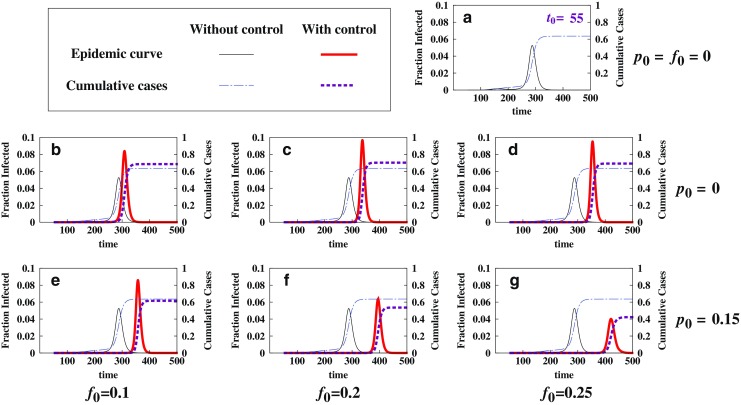
Comparison of epidemic severity for different combinations of p ₀ and f ₀. This figure illustrates the effect of treatment when combined with vaccination. The model used is (2.5) with initial conditions (2.6), where I _u0 = 1 and N = 305 million; a is again for the case of no control (f ₀ = p ₀ = 0) and for t ₀ = 55; b–d are for the case of no vaccination (p ₀ = 0), whereas e–g are for the case in which an intermediate level of vaccination (p ₀ = 0.15) is applied with a starting time t _v = 150. We observe that together with vaccination, antiviral drugs will be more beneficial

Figure 10 illustrates the effect of drug treatment either used alone (i.e., f₀  > 0 and p₀ = 0) or combined with vaccination (i.e., f₀  > 0 and p₀  > 0). For demonstration purposes, it is chosen that t₀ = 55. Figure 10a is for the case of no control (f₀ = p₀ = 0). By comparing the panels in the middle (p₀ = 0) and the bottom (p₀  > 0) we observe that although antiviral use may increase the peak and final sizes when used alone, its benefit can be dramatically improved when combined with the use of vaccination.

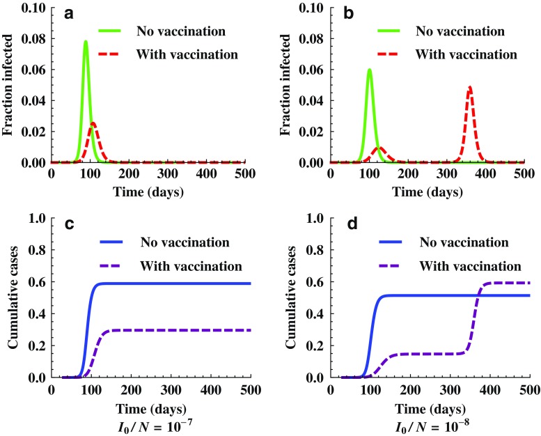
Another factor that may also affect the final pandemic size is the initial fraction of infected individuals I₀/N at t₀. Figure 11 shows the outcomes of the model (2.5) for two different initial values of I₀/N. Other parameter values used are β = 0.35, γ = 1/3, f₀ = 0, p₀ = 0.1, t₀ = 30, and t_v = 0. Again, it shows that the outcomes can be sensitive to the initial values. Particularly, although vaccination reduced the peak and final sizes (see a and c) for the case of I₀/N = 10⁻⁷, the use of vaccination actually increased the final size for the case of I₀/N = 10⁻⁸ (see b and d).

Fig. 11.

Simulations showing the effect of initial conditions. It demonstrates changes in epidemic outcomes for two different values of initial fraction of infected individuals, I ₀ /N = 10⁷ (a and c) and I ₀ /N = 10⁸ (b and d). The model used is (2.5) with f ₀ = 0, p ₀ = 0.1, t ₀ = 30, and t _v = 0. We observe that for the case of I ₀ /N = 10⁸, a second wave occurred around t = 350 and the final cumulative infections with vaccination is higher than that without vaccination

Implications for Policy Decisions in Public Health

As mentioned earlier, effective control strategies for pandemics should aim at lowering the peak size to lest demand for facilities exceed supply, lowering the final size to reduce morbidity and delaying the peak to provide time for response. However, results presented here show that an increase in control efforts may not always be beneficial for achieving these objectives. Particularly, the outcomes demonstrated in Figs. 7, 8, 9, 10, and 11 suggest that in some cases, the uses of vaccine and treatment may have a detrimental consequence (e.g., increasing peak and/or final epidemic sizes), and that whether and how much vaccination and treatment can be helpful will depend critically on the time of introduction of infection (t₀), the starting time of vaccination use (t_v), and the levels of vaccination and treatment (p₀ and f₀). Thus, it is very important that these control programs are designed appropriately.

A possible explanation for the negative effects of these control measures is the seasonal variation disease transmission. Vaccination/treatment during the spring wave of an epidemic essentially increases susceptibles at the end of the summer. This larger number of susceptibles can, in some cases, act as tinder for a much larger epidemic to occur in the more favorable influenza season of autumn than may have occurred if treatment had not been used in the summer months. Thus, to increase the likelihood of successful control programs, policy decisions should take into consideration the potential impact of these factors on disease transmission dynamics.

DISCUSSION

In this paper, we use simple SIR-type epidemic models to study the effect of vaccination and antiviral use on the control and prevention of infectious diseases. Model analyses and simulations are carried out using parameter values related to influenza. The models are simple in the sense that they do not include many of the heterogeneities that may affect disease dynamics. These heterogeneities include age-dependent transmission rate, multiple viral strains (including drug-resistant strains), age or spatial variations in contact patterns, etc. We have previously studied the effects of some of these heterogeneities on the disease dynamics (2,11–14). The results presented here suggest that although vaccination and drug treatment will help reduce the disease prevalence in the case of constant transmission rate, their benefits can be compromised if the transmission rate is seasonally forced.

To demonstrate this through modeling, we compared results of epidemic models with and without vaccination and/or treatment, which helped us to examine how the timing and levels of disease control programs may influence the model outcomes in terms of the peak and final sizes of a pandemic. We demonstrated that when the transmission rate β is constant and when vaccination and treatment are available at the beginning of an epidemic, the disease prevalence always decreases with control efforts by increasing the proportion of population vaccinated and/or treated, and by improving the efficacy of vaccines. The main reason for this is that in this case, the control efforts will reduce the reproduction number , which determines the severity of the disease outbreak (see Figs. 3, 5, and 6).

The situation when β(t) incorporates seasonal variations can differ dramatically. Particularly, the model results suggest that the effectiveness of control programs can be very sensitive to the model parameters representing various control measures. We illustrated several scenarios in which the uses of vaccination or treatment may actually increase peak and final epidemic sizes (see Figs. 8, 9, and 10). Although more theoretical studies are needed to better understand how periodic forcing may affect the disease dynamics in general, some preliminary observations can be made based on our simulations.

SIR models with periodic transmission rates (β(t)) are extremely non-linear and the final size of the epidemic is strongly dependent upon the initial conditions such as the time of introduction (t₀) of the pathogens into the population, the initial proportion of susceptibles and infectious (S₀ and I₀, see Fig. 11). Particularly, periodic SIR models can produce epidemic curves with more than one peak; depending on values of mode parameters such as t₀ and ε, the spring epidemic may not reduce the number of susceptibles sufficiently to prevent the epidemic from once again taking off in the autumn (during a favorable time of year when β(t) begins to rise again).

In summary, our model studies suggest that the patterns of disease transmission (e.g., with or without seasonal variations) can have a significant influence on the effectiveness of control and intervention programs. When a disease exhibits periodic patterns in transmission, decisions of public health policies will be particularly important as to how control measures such as vaccination and drug treatment should be implemented. More importantly, mathematical models can be very helpful for understanding complex disease transmission dynamics and for identifying the optimal control strategies.

References

- 1.Anderson RM, May RM. Infectious diseases of humans: dynamics and control. Oxford: Oxford University Press; 1991. [Google Scholar]
- 2.Glasser JW, Taneri D, Feng Z, Chuang J-H, Tll P, et al. Evaluation of targeted influenza vaccination strategies via population modeling. PLoS ONE. 2010;5(9):e12777. doi: 10.1371/journal.pone.0012777. [DOI] [PMC free article] [PubMed] [Google Scholar]
- 3.Fraser C, et al. (H1N1): early findings pandemic potential of a strain of influenza A. Science. 2009;324:1557. doi: 10.1126/science.1176062. [DOI] [PMC free article] [PubMed] [Google Scholar]
- 4.Gani R, et al. Potential impact of antiviral use during influenza pandemic. Emerg Infect Dis. 2005;11(9):1355–1362. doi: 10.3201/eid1109.041344. [DOI] [PMC free article] [PubMed] [Google Scholar]
- 5.Lipsitch M, Cohen T, Muray M, Levin BR. Antiviral resistance and the control of pandemic influenza. PLoS Med. 2007;4:01110120. doi: 10.1371/journal.pmed.0040015. [DOI] [PMC free article] [PubMed] [Google Scholar]
- 6.Medlock J, Galvani AP. Optimizing influenza vaccine distribution. Science. 2009 doi: 10.1126/science.1175570. [DOI] [PubMed] [Google Scholar]
- 7.Towers S, Feng Z. Pandemic H1N1 influenza: predicting the course of pandemic and assessing the efficacy of the planned vaccination programme in the United States. Eurosurveillance. 2009;14(41):6–8. [PubMed] [Google Scholar]
- 8.Washington Times (11/20/2009). Study: H1N1 vaccine too late to help most. http://www.washingtontimes.com/news/2009/oct/20/study-swine-flu-vaccine-too-late-to-help-most/. Accessed 1 June 2011.
- 9.U.S. Centers for Disease Control: Weekly Influenza Surveillance Report 2009–2010 Influenza Season. http://www.cdc.gov/flu/weekly/weeklyarchives2009–2010/weekly20.htm/. Accessed 1 June 2011.
- 10.Renshaw E. Modelling biological populations in space and time. Cambridege: Cambridge University Press; 1993. [Google Scholar]
- 11.Glasser JW, Feng Z, Moylan A, Del Valle S, Castillo-Chavez C. Mixing in age-structured population models of infectious diseases. 2011 (in review). [DOI] [PubMed]
- 12.Qiu Z, Feng Z. Transmission dynamics of an influenza model with vaccination and antiviral treatment. Bull Math Biol. 2010a;72(1):1–33. doi: 10.1007/s11538-009-9435-5. [DOI] [PubMed] [Google Scholar]
- 13.Qiu Z, Feng Z. Transmission dynamics of an influenza model with age of infection and antiviral treatment. J Dyn Diff Equat. 2010b doi: 10.1007/s11538-009-9435-5. [DOI] [PubMed] [Google Scholar]
- 14.Qiu Z, Feng Z. Dynamics of an epidemic model with targeted antiviral prophylaxis. JBD. 2010c;4(5):506–526. doi: 10.1080/17513758.2010.498925. [DOI] [PubMed] [Google Scholar]