

Abstract
This paper presents a data-centric modeling and predictive control approach for nonlinear hybrid systems. System identification of hybrid systems represents a challenging problem because model parameters depend on the mode or operating point of the system. The proposed algorithm applies Model-on-Demand (MoD) estimation to generate a local linear approximation of the nonlinear hybrid system at each time step, using a small subset of data selected by an adaptive bandwidth selector. The appeal of the MoD approach lies in the fact that model parameters are estimated based on a current operating point; hence estimation of locations or modes governed by autonomous discrete events is achieved automatically. The local MoD model is then converted into a mixed logical dynamical (MLD) system representation which can be used directly in a model predictive control (MPC) law for hybrid systems using multiple-degree-of-freedom tuning. The effectiveness of the proposed MoD predictive control algorithm for nonlinear hybrid systems is demonstrated on a hypothetical adaptive behavioral intervention problem inspired by Fast Track, a real-life preventive intervention for improving parental function and reducing conduct disorder in at-risk children. Simulation results demonstrate that the proposed algorithm can be useful for adaptive intervention problems exhibiting both nonlinear and hybrid character.
Index Terms: Nonlinear hybrid systems, Model Predictive Control, Model-on-Demand, optimized behavioral interventions
I. Introduction
Hybrid systems are characterized by interaction between continuous and discrete dynamics [1], [2]. In recent years, significant emphasis has been given to modeling and control of nonlinear hybrid systems based on first principles models [2], [3], [4]. However, this is only useful for small and well understood systems. On the other hand, data-driven modeling is critical in many practical applications. Consider, for example, adaptive interventions in behavioral health, which are receiving increasing attention as a means to address the prevention and treatment of chronic, relapsing disorders such as drug abuse [5]. In an adaptive intervention, dosages of intervention components are assigned based on the values of tailoring variables that reflect some measure of outcome or adherence. In practice, these problems are hybrid in nature because dosages of intervention components correspond to discrete values. The dynamics of these systems can be complex and highly uncertain, with many factors that contribute to these dynamics not well understood. Moreover, these interventions have to be implemented on a population or cohort that may display significant levels of interindividual variability. Thus, a data-driven modeling and control formulation which achieves robust performance is essential. This paper is an attempt to focus on these issues for nonlinear hybrid systems.
Identification theory for continuous systems is well understood in the literature (see for example [6]). However, hybrid system identification is challenging due to presence of discrete events. A number of identification approaches for linear hybrid systems have been proposed in the literature [7], [8], [9], [10]. An identification scheme for nonlinear hybrid systems has been presented in [11]. However, it addresses only a particular class of nonlinear hybrid systems which are linear and separable in the discrete variables. Moreover, locations or modes of the hybrid systems are assumed to be known beforehand. There has been significant interest in data-centric dynamic modeling frameworks such as Just-in-Time modeling [12], Model-on-Demand (MoD) estimation [13], [14] and more recently, Direct Weight Optimization (DWO) [15] for continuous systems. These modeling approaches enable nonlinear estimation and can be a promising approach for identification of nonlinear hybrid systems.
This paper presents a Model-on-Demand Predictive Control (MoDPC) formulation for nonlinear hybrid systems. The proposed scheme represents a significant extension of earlier work by the authors [4] which develops a model predictive control (MPC) formulation for hybrid systems that is amenable for achieving robust performance. This MPC formulation offers a multiple-degree-of-freedom tuning arrangement that enables the user to adjust the speed of setpoint tracking, measured disturbance rejection and unmeasured disturbance rejection independently in the closed-loop system. Consequently, controller tuning is more flexible and intuitive than relying on move suppression weights as traditionally used in MPC schemes. The work in this paper extends this MPC formulation to the control of nonlinear hybrid systems that involve both state and control events using a data-centric MoD approach. In this approach, the MoD estimator is executed at each sampling instant in order to generate a linear local polynomial model at the current operating point from a subset of available data as determined by a crossvalidation data measure. This model is then converted into a mixed logical and dynamical (MLD) model [1] for linear hybrid systems, which is used by the multiple-degree-of-freedom MPC algorithm [4]. By systematically achieving model estimation from data through the MoD algorithm, without substantially increasing computational burden or increasing problem complexity, the hybrid MoDMPC approach described in this paper has the potential to make this integrated modeling and control much more accessible in practice.
The paper is organized as follows: Section 2 develops the identification scheme for nonlinear hybrid systems using MoD approach. MoDMPC formulation for nonlinear hybrid systems is presented in Section 3. Section 4 discuss a case study problem of a hypothetical adaptive intervention based on Fast Track program and simulation results. A summary and conclusions is presented in Section 5.
II. Identification of nonlinear hybrid system using Model-on-Demand approach
Consider a nonlinear hybrid system that can be described by following set of differential algebraic equations,
| (1) |
| (2) |
| (3) |
where x represents a vector for states, u is a vector for inputs (both continuous and discrete), y is the measured outputs, and function vector G[·] is a set of event generating functions. The function G[·] can be classified into an autonomous event generating function which is governed by the states of the system (i.e. G[x]) and a non-autonomous (or deterministic) event generating function that governed by the inputs and the outputs of the system (i.e. G[u(t), y(t)]). In (2), ‘s’ represents the discrete variables that can take finite integer values evaluated by G[·]. Upon occurrence of an event, ‘s’ takes a new value and the hybrid system transits from one location (or mode) to anther. Thus, a new value of ‘s’ corresponds to a new location of the hybrid system. Each of these locations is governed by individual nonlinear dynamics characterized by states and inputs of the system. The challenge in the identification of hybrid systems lies in the fact that the model parameters depend on the mode or location [11], [9]. In case of hybrid systems with only non-autonomous (or deterministic) events, locations of the subsystems are known a priori, and the identification problem consists of estimating model parameters for all locations. In the presence of autonomous events, the identification problem requires the simultaneous identification of location (or mode) of the system and estimation of model parameters, which is difficult problem to solve due to its mixed integer and nonlinear nature.
A Model-on-Demand (MoD) approach [16] that generates a model “on demand” relevant to the region of interest using subset of neighborhood data around current operating point can be an useful tool for identification of such systems. Model-on-Demand is a data-centric, nonlinear black-box estimation method which enhances the classical local modeling problem. In MoD, an adaptive bandwidth selector determines the size of data to be used for the local regression. The data is weighted using a kernel or weighting function. A local regression is performed using a linear or quadratic model to estimate the plant output at each time step; all observations are stored on a database and the models are built ‘on demand’ as the actual need arises. Local modeling techniques such as the MoD predictor use only small portions of data, relevant to the region of interest around current operating point defined by regressors, to determine a model. Thus, MoD automatically considers the current operating location of the hybrid system and correspondingly estimates the model parameters. The variance/bias tradeoff inherent to all modeling is optimized locally by adapting the number of data and their relative weighting. As a consequence, the non-convex and mixed integer optimization problem associated with global modeling of nonlinear hybrid systems can be avoided. A Matlab-based tool for MoD estimation is available in the public domain [17].
A. Model on Demand Estimation
The MoD modeling formulation is described with a SISO process based on the approach of [16]. Consider a SISO process with nonlinear ARX structure, i.e.,
| (4) |
where m(·) is an unknown nonlinear mapping and e(k) is an error term modeled as random variables with zero mean and variance . The MoD predictor attempts to estimate output predictions based on a local neighborhood of the regressor space φ(t). The regressor vector is of the form
| (5) |
where na, nb, and nk denote the number of previous outputs and inputs and the degree of delays in the model.
A local estimate ŷ can be obtained from the solution of the weighted regression problem
| (6) |
where l(·) is a quadratic norm function, is a scaled distance function on the regressor space, h is a bandwidth parameter controlling the size of the local neighborhood, which is determined via Akaike’s FPE criteria and W(·) is a window function (usually referred to as the kernel) assigning weights to each remote data point according to its distance from φ(t) [16]. The window is typically a bell-shaped function with bounded support. These weights can be chosen to minimize the point-wise mean square error of the estimate. Assuming a local model structure
| (7) |
which is linear in the unknown parameters, an estimate can easily be computed using least squares methods. If β̂0 and β̂1 denote the minimizers of (6) using the model from (7), a one-step ahead prediction is given by
| (8) |
where . Each local regression problem produces a single prediction ŷ(k) corresponding to the current regression vector φ(t). To obtain predictions at other operating points in the regressor space, the weights change and a new optimization problem must be solved. This stands in contrast to the global modeling approach where the model is fitted to data only once and then discarded. The bandwidth h controls the neighborhood size and critically impacts the resulting estimate since it governs the tradeoff between bias and variance errors of the estimate. Traditional bandwidth selectors produce a single global bandwidth; in MoD estimation, a bandwidth is computed adaptively at each prediction.
B. From time series MoD model to MLD model
A standard practice in obtaining MIMO models involves performing identification for each individual output of the system (as described above) and stacking these together to obtain a MIMO model comprising multiple linear polynomials (one for each output) of the form (8). This polynomial model can be rearranged in the following piecewise affine (PWA) form:
| (9) |
| (10) |
Here A, B1 and C are state space matrices that can be generated from the elements of β1, while f is a constant affine term derived from α. d′ and ν represent unmeasured disturbances and measurement noise signals, respectively. Because disturbances are an inherent part of any process, it is necessary to incorporate these in the controller model that defines the control system. It should be noted that the matrices A, B1, C and f vary at each time step based on current operating point. Hence the effect of the autonomous events are automatically captured and the model represents the dynamics of current location of the system. At this stage, any deterministic logical condition on inputs or outputs (i.e. non-autonomous events) can be included in the model. These logical conditions are than converted into linear constraints to obtain the standard MLD form [1] given below:
| (11) |
| (12) |
| (13) |
δ and z are discrete and continuous auxiliary variables that are introduced in order to convert logical/discrete decisions into their equivalent linear inequality constraints summarized in (13) (for details, see [1]).
III. Model-on-Demand Predictive Control for Hybrid Systems
The MLD model (11)-(13) estimated through a MoD approach is used to formulate the hybrid model predictive control (MPC) law presented in [4]. The controller model (11)-(13) lumps the effect of all unmeasured disturbances on the outputs only, which is a common practice in the process control literature [18]. We consider d′, the unmeasured disturbance, as a stochastic signal, described as follows,
| (14) |
| (15) |
where Aw has all eigenvalues inside the unit circle and w(k) is a vector of integrated white noise. Here, it is assumed that the disturbance effect is uncorrelated. Thus, Bw = Cw = I and Aw = diag{α1, α1, ⋯ , αny} where ny is number of outputs. In order to take advantage of well understood properties of white noise signal considering difference form of disturbance and system models and augmenting them as follows,
| (16) |
| (17) |
Here and Δw(k) is white noise sequence. Augmented matrices A , ℬi (i = 1, 2, 3) and C are given in [4].
A. MPC Problem
In this work, we use a quadratic cost function of the form,
| (18) |
subjected to mixed integer constraints according to (13) and various process and safety constraints,
| (19) |
| (20) |
| (21) |
p is the prediction horizon and m is the control horizon. umin, umax, Δumin, Δumax, and ymin, ymax are lower and upper bound on inputs, move sizes, and outputs, respectively. (·)r stands for reference trajectory and ∥·∥2 is for 2-norm. Qy, QΔu, Qu, Qd, and Qz are penalty weights on the control error, move size, control signal, auxiliary binary variables and auxiliary continuous variables, respectively.
The MPC problem (18)-(21) is governed by both binary and continuous decision variables hence it is a mixed integer quadratic program (miqp). Moreover, it requires future predictions of the outputs and the mixed integer constraints in (13), which can be obtain by propagating (13), (16) and (17) for p steps in future. These multi-step predictions are then used to convert aforementioned MPC problem to a standard miqp (for details, see [4]). This problem can be solved using any miqp solver available in the market. In this work, we have used the Tomlab-CPLEX solver. It should be noted that the algorithm also requires externally generated reference trajectories and estimate of (disturbance free) initial states X(k) that influence the robust performance of the proposed formulation.
The output reference trajectory is generated using an asymptotically step (a Type-I filter per [19]) as follows,
| (22) |
The setpoint tracking speed can be adjusted by choosing between [0,1) for each individual output. The smaller the value for , the faster the response for particular setpoint tracking. Thus, setpoint tracking speed can be adjusted for each output individually.
The states of the system can be estimated from the current measurements, y(k) while rejecting the unmeasured disturbance using a Kalman filter as follows:
| (23) |
| (24) |
Here Kf is the filter gain, an optimal value of which can be found by solving an algebraic Riccati equation. We use the parametrization of filter gain [18] as follows,
| (25) |
where
| (26) |
| (27) |
| (28) |
(fa)j is a tuning parameter that lies between 0 and 1. While the unmeasured disturbances are rejected using the state observer presented in (23)-(28), the speed of rejection is proportional to the tuning parameter (fa)j. As (fa)j approaches zero, the state estimator increasingly ignores the prediction error correction, and the control solution is mainly determined by the deterministic model, (23). On the other hand, the state estimator tries to compensate for all prediction error as (fa)j approaches to 1, with a corresponding increase in the aggressiveness of the control action. In practice, the judicious selection of (fa)j requires making the proper tradeoff between performance and robustness.
IV. Case Study: Adaptive Interventions
As a representative case study of a time-varying adaptive behavioral intervention we examine the Fast Track program [20]. Fast Track was a multi-year, multi-component program designed to prevent conduct disorders in at-risk children. Youth showing conduct disorder are at increased risk for incarceration, injury, depression, substance abuse, and death by homicide or suicide. In Fast Track, some intervention components were delivered universally to all participants, while other specialized components were delivered adaptively. In this paper we focus on a hypothetical adaptive intervention described in [5] for assigning family counseling, which was provided to families on the basis of parental functioning. There are several possible levels of intensity, or doses, of family counseling. The idea is to vary the doses of family counseling depending on the needs of the family, in order to avoid providing an insufficient amount of counseling for very troubled families, or wasting counseling resources on families that may not need them or be stigmatized by excessive counseling. The decision about which dose of counseling to offer each family is based primarily on the family’s level of functioning, assessed by a family functioning questionnaire completed by the parents. As described in [5], based on the questionnaire and the clinician’s assessment, family functioning is determined to fall in one of the following categories: very poor, poor, near threshold, or at/above threshold. A corresponding decision rule that can be applied is as follows: families with very poor functioning are given weekly counseling; families with poor functioning are given biweekly counseling; families with near threshold functioning are given monthly counseling; and families at or above threshold are given no counseling. Family functioning is reassessed at a review interval of one months, at which time the intervention dosage may change. This goes on for four years.
Rivera et al. [21] analyzed the intervention by means of a fluid analogy, represented in Figure 1. Parental function PF(k) is treated as fluid in a tank, which is depleted by exogenous disturbances D(k). The tank is replenished by the intervention I(k), which is the manipulated variable. The use of fluid analogy enables developing a mathematical model of the open-loop dynamics of the intervention using the principle of conservation of mass. This model can be described by nonlinear difference equations which relates parental function PF(k) with the intervention I(k) as follows:
| (29) |
| (30) |
| (31) |
PF(k) is parental function, I(k) refers to the intervention dosage (frequency of counselor home visits), KI(k) is the time-varying intervention gain, T represent the review period or sampling time (= 1 month), θ(k) represents the time-varying time delay between intervention and its effect on parental function, PFmeas(k) is the parental function measurement. D(k) is the source of parental function depletion and N(k) represents the measurement noise. Here we consider both nonlinear gain and delay relationships. The gain, KI varies with parental function PF(k) as follows,
| (32) |
where c = Kmax − b and . A graphical representation of this relationship for Kmax = 0.3, Kmin = 0.06, a = 10 is shown in Fig. 2. The delay θ varies with parental function PF(k) per the following rules:
| (33) |
Moreover, the intervention I(k) has a restriction on the frequency of counselor visits, which requires imposing a restriction on the intervention I(k) such that it takes only four values: 0, Iweekly, Ibiweekly and Imonthly. Hence the problem has inherent discreteness that can be classified as non-autonomous (deterministic) discrete events in addition to the continuous dynamics. Thus, system can be characterized by the nonlinear hybrid dynamical system.
Fig. 1.
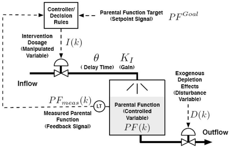
Fluid analogy corresponding to the hypothetical adaptive intervention. Parental function PF(k) is treated as material (inventory) in a tank, which is depleted by disturbances D(k) and replenished by intervention dosage I(k), which is the manipulated variable.
Fig. 2.
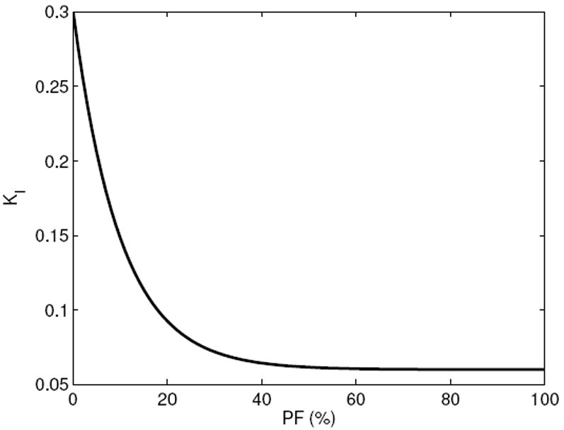
Graphical depiction of the nonlinear gain relationship given in Equation 32 for KI.
In the case study an implicit NARX structure with [na = 2, nb = 2, nk = 1] is used in the MoD estimator. A first order local polynomial and database size limit [50 240] is used as additional parameters. This local model is then converted into its equivalent state-space form described by (9)-(10). Further, in order to capture deterministic discrete events in the intervention, four binary auxiliary variables, δ1, δ2, δ3, δ4 and four continuous auxiliary variables, I1, I2, I3, I4 are introduced and the equivalent MLD model per (11)-(13) is obtained. The detailed description of the MLD model is not presented here for the sake of brevity. This model is generated adaptively at each time step and used to formulate the MPC problem.
Figure 3 compares the open-loop simulation results using the MoD approach (dashed line) with the open-loop simulation from the actual nonlinear system (29)-(33) (solid line). It can be seen that the MoD approach satisfactorily estimates the dynamic behavior of the system with root mean square (RMS) error 5.62. On the other hand, the simulation result from the linear ARX model using the same model structure as the MoD model (denoted by dotted line in Fig. 3), yields a poor estimation result with RMS error value of 13.68.
Fig. 3.
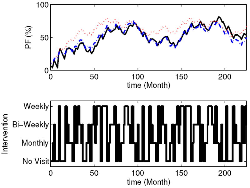
Comparison with open-loop simulation using MoD model (dashed line) and linear ARX model (dotted line) with nonlinear systems (solid line).
Figure 4 documents the MPC performance using the MoD approach (solid line) with the linear ARX model approach (dashed-dotted line) in the presence of a setpoint change in parental function to 65% and a simultaneous step unmeasured disturbance D(k) = 4. In both the cases, the MPC tuning parameters Qy = 1, QΔu = 0.1, Qu = Qd = Qz = 0, (αr, fa) = (0, 0.3), the prediction horizon p = 40 and control horizon m = 10 are used. The Tomlab-CPLEX solver is used to solve resulting miqp optimization problems. From the figure it can be seen that the controller designed using the MoD approach is able to quickly achieve the desired setpoint, and stabilizes the system at the setpoint. In contrast, the controller relying on the linear ARX model oscillates around setpoint. In addition, the proposed algorithm produces less variation in the manipulated variable and provides uniform performance. This fact is also confirmed by the performance matrices Je and JΔI given below:
| (34) |
| (35) |
where t represents total simulation time and Ts is a sampling time. The performance matrices Je and JΔI represent measure of cumulative deviation of parental function from the goal and measure of cumulative variation in the intervention dosages, respectively. For the MoD approach, values of Je and JΔI are 7.84 × 10³ and 1.11 × 10⁴, respectively, while using the linear ARX model based MPC, these values are 9.05 × 10³ and 1.55 × 10⁴, respectively. Thus, it can be concluded that the proposed algorithm yields superior performance and is suitable for the control of nonlinear hybrid systems.
Fig. 4.
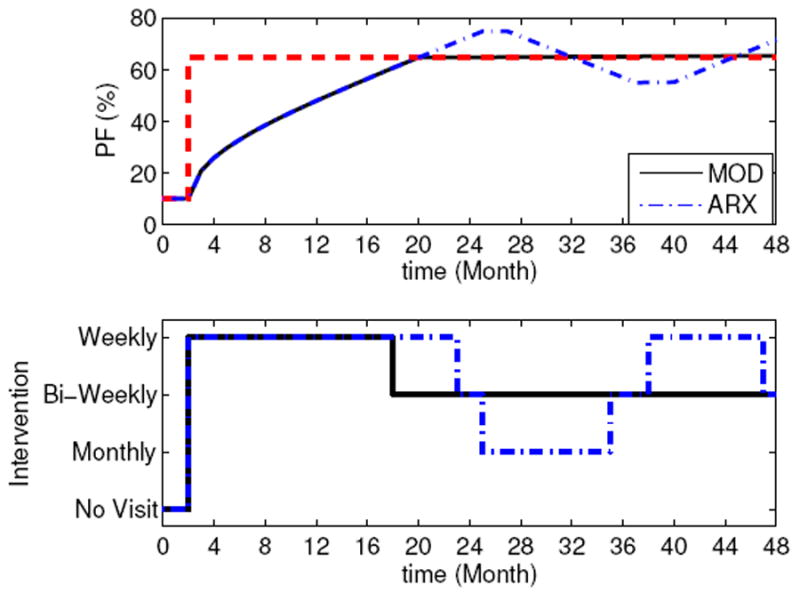
Comparison of controller performance using the proposed MoD-MPC formulation (solid line) and the MPC formulation relying on linear ARX model (dashed-dotted line). A setpoint change from 10% to 65% parental function with simultaneous step disturbance D(k) = 4 are evaluated with tuning parameter Qy = 1, QΔu = 0.1, Qu = Qd = Qz = 0, (αr, fa) = (0, 0.3), p = 40 and m = 10.
V. Summary
Applications of hybrid systems are becoming increasingly common in many fields. Recently, control engineering principles have been proposed for adaptive behavioral interventions [21]; these systems are naturally hybrid in nature. In this work, a Model-on-Demand Predictive Control (MoDPC) approach for control of nonlinear hybrid systems and its application to a simulated adaptive behavioral intervention are presented. The formulation uses a Model-on-Demand approach to obtain a local MLD model for the nonlinear hybrid system at each time step. MoD is a data-centric approach that uses a small neighborhood data around current operating point characterized by the regressor vector. The local MLD model generated by MoD estimator is then used to specify a model predictive control law that relies on multiple-degree-of-freedom tuning parameters [4]. Multiple-degree-of freedom tuning enables the speed of disturbance rejection and setpoint tracking affecting each output to be adjusted individually; this has intuitive appeal. The applicability and efficiency of proposed formulation is demonstrated on a hypothetical intervention problem intended for improving parental function in at-risk children. This problem exhibits nonlinear dynamics with inherent discrete events. From the simulation results, it can be concluded that the proposed MoDPC is useful for the control of nonlinear hybrid systems, displaying acceptable performance levels while simplifying the task of modeling.
Acknowledgments
Support for this work has been provided by the Office of Behavioral and Social Sciences Research (OBSSR) of the National Institutes of Health and the National Institute on Drug Abuse (NIDA) through grants K25 DA021173 and R21 DA024266. Insights provided by Linda M. Collins (Methodology Center, Penn State University) and Susan A. Murphy (University of Michigan) towards better understanding adaptive behavioral interventions are greatly appreciated.
Contributor Information
Naresh N. Nandola, Email: nnandola@asu.edu.
Daniel E. Rivera, Email: daniel.rivera@asu.edu.
References
- 1.Bemporad A, Morari M. Control of systems integrating logic, dynamics, and constraints. Automatica. 1999;35(3):407–427. [Google Scholar]
- 2.Nandola NN, Bhartiya S. A multiple model approach for predictive control of nonlinear hybrid systems. J Process Control. 2008;18(2):131–148. [Google Scholar]
- 3.Nandola NN, Bhartiya S. A computationally efficient scheme for model predictive control of nonlinear hybrid systems using generalized outer approximation. Ind Eng Chem Res. 2009;48(12):5767–5778. [Google Scholar]
- 4.Nandola NN, Rivera DE. ACC. FrC01.5. Baltimore, Maryland, USA: Jun 30 02, Jul 30 02, 2010. A novel model predictive control formulation for hybrid systems with application to adaptive behavioral interventions; pp. 6286–6292. [DOI] [PMC free article] [PubMed] [Google Scholar]
- 5.Collins LM, Murphy SA, Bierman KL. A conceptual framework for adaptive preventive interventions. Prevention Science. 2004;5(3):185–196. doi: 10.1023/b:prev.0000037641.26017.00. [DOI] [PMC free article] [PubMed] [Google Scholar]
- 6.Ljung L. System Identification Theory For the User. second. PTR Prentice Hall; New Jersey: 1999. [Google Scholar]
- 7.Vidal R. Recursive identification of switched ARX systems. Automatica. 2008;44(9):2274–2287. [Google Scholar]
- 8.Egbunonu P, Guay M. Identification of switched linear systems using subspace and integer programming techniques. Nonlinear Anal Hybrid Syst. 2007;1(4):577–592. [Google Scholar]
- 9.Roll J, Bemporad A, Ljung L. Identification of piecewise affine systems via mixed-integer programming. Automatica. 2004;40(1):37–50. [Google Scholar]
- 10.Ferrari-Trecate G, Muselli M, Liberati D, Morari M. A clustering technique for the identification of piecewise affine systems. Automatica. 2003;39(2):205–217. [Google Scholar]
- 11.Nandola NN, Bhartiya S. Hybrid system identification using a structural approach and its model based control: An experimental validation. Nonlinear Anal Hybrid Syst. 2009;3(2):87–100. [Google Scholar]
- 12.Cybenko G. Just-in-time learning and estimation. In: Bittani S, Picci G, editors. Identification, Adaptation, Learning, NATO ASI. Springer; 1996. pp. 423–434. [Google Scholar]
- 13.Braun M. PhD thesis. Arizona State University; USA: 2001. Model-on-demand nonlinear estimation and model predictive control: Novel methodologies for process control and supply chain management. [Google Scholar]
- 14.Stenman A. PhD thesis. Linkoping University; Sweden: 1999. Model on demand: Algorithms, analysis and applications. [Google Scholar]
- 15.Roll J, Nazin A, Ljung L. Nonlinear system identification via direct weight optimization. Automatica. 2005;41(3):475–490. Data-Based Modelling and System Identification. [Google Scholar]
- 16.Braun M, Rivera DE, Stenman A. A model-on-demand identification methodology for nonlinear process systems. Int J Control. 2001;74(18):1708–1717. [Google Scholar]
- 17.Braun M, Stenman A, Rivera DE. Model-on-demand model predictive control toolbox. 2002 http://csel.asu.edu/MoDMPCtoolbox.
- 18.Lee JH, Yu ZH. Tuning of model predictive controllers for robust performance. Comput Chem Eng. 1994;18(1):15–37. [Google Scholar]
- 19.Morari M, Zafiriou E. Robust Process Control. Englewood Cliffs, NJ: Prentice-Hall; 1989. [Google Scholar]
- 20.Conduct Problems Prevention Research Group. A developmental and clinical model for the prevention of conduct disorders: The Fast Track program. Development and Psychopathology. 1992;4:509–528. [Google Scholar]
- 21.Rivera DE, Pew MD, Collins LM. Using engineering control principles to inform the design of adaptive interventions a conceptual introduction. Drug and Alcohol Dependence. 2007;88(2):S31–S40. doi: 10.1016/j.drugalcdep.2006.10.020. [DOI] [PMC free article] [PubMed] [Google Scholar]