Automated vector selection of SIVQ and parallel computing integration MATLAB™: Innovations supporting large-scale and high-throughput image analysis studies

Abstract

Introduction:

Spatially invariant vector quantization (SIVQ) is a texture and color-based image matching algorithm that queries the image space through the use of ring vectors. In prior studies, the selection of one or more optimal vectors for a particular feature of interest required a manual process, with the user initially stochastically selecting candidate vectors and subsequently testing them upon other regions of the image to verify the vector's sensitivity and specificity properties (typically by reviewing a resultant heat map). In carrying out the prior efforts, the SIVQ algorithm was noted to exhibit highly scalable computational properties, where each region of analysis can take place independently of others, making a compelling case for the exploration of its deployment on high-throughput computing platforms, with the hypothesis that such an exercise will result in performance gains that scale linearly with increasing processor count.

Methods:

An automated process was developed for the selection of optimal ring vectors to serve as the predicate matching operator in defining histopathological features of interest. Briefly, candidate vectors were generated from every possible coordinate origin within a user-defined vector selection area (VSA) and subsequently compared against user-identified positive and negative “ground truth” regions on the same image. Each vector from the VSA was assessed for its goodness-of-fit to both the positive and negative areas via the use of the receiver operating characteristic (ROC) transfer function, with each assessment resulting in an associated area-under-the-curve (AUC) figure of merit.

Results:

Use of the above-mentioned automated vector selection process was demonstrated in two cases of use: First, to identify malignant colonic epithelium, and second, to identify soft tissue sarcoma. For both examples, a very satisfactory optimized vector was identified, as defined by the AUC metric. Finally, as an additional effort directed towards attaining high-throughput capability for the SIVQ algorithm, we demonstrated the successful incorporation of it with the MATrix LABoratory (MATLAB™) application interface.

Conclusion:

The SIVQ algorithm is suitable for automated vector selection settings and high throughput computation.

INTRODUCTION

Vector Quantization is an established and well-known technique,[1–3] and its lack of rotation invariance with respect to extracted features from images has similarly been considered.[4,5] Spatially invariant vector quantization (SIVQ) is a pattern recognition algorithm that has been described recently.[6] SIVQ differs fundamentally from other image analysis algorithms in its use of rings to represent image predicate features. By taking advantage of the continuous symmetry inherent in the ring structure, SIVQ is able to identify the predicate features independent of the stochastic variance posed by features possessing arbitrary rotational orientations.[6] Of late, it has been integrated as a turnkey solution, supporting high-throughput laser capture microdissection (LCM)[7] with this construct affording the retrieval of significantly augmented quantities of tissue over conventional manual selection means.

Prior to this report, vector selection using the SIVQ discovery tool software suite involved an iterative process where manual trial selection of candidate vectors was required until one was found that exhibited suitable sensitivity and specificity. Inherent in this manual process was the lack of a formalized tool suite or programmatic solution for visualizing the receiver-operator characteristics of each candidate vector, making side-by-side performance comparisons of each candidate vector difficult, if not impossible.

In this work, we report a method by which each iteratively selected vector from the VSA is iteratively tested against all possible search positions in the test areas of the remaining image surface area, with sensitivity and specificity being assessed by review of the ROC/AUC-provided goodness-of-match heat map. A functional evaluation of this process underscored the tedious and stochastic nature of obtaining high-performance vectors, even in the setting of benefitting from a histopathological subject matter expert.

Here we introduce two new features to SIVQ workflow. The first is a fully automated selection process to yield optimal vectors without iterative manual discovery. Secondly, we demonstrate a complete rendering of the SIVQ algorithm within a parallel computation environment, via the use of the MATLAB™ application programming interface (API). Collectively, these two innovations render the SIVQ algorithm as being more suitable for actual clinical deployment, by virtue of both newly-gained automation and speed, respectively.

MATERIALS AND METHODS

For a detailed description of the SIVQ algorithm, the reader is referred to Hipp and Cheng et al.[6] In this study, the previously described computational method is itself unchanged, with the primary differences being: (1) addition of an iterative and automated vector selection process, and (2) implementation of the core algorithm on a symmetric multiprocessor platform, via the use of MATLAB™.

Spatially Invariant Vector Quantization algorithm Modification

Automatic vector selection

An additional application module was written in Visual Basic (Visual Studio, Microsoft Corporation) and added to the vector discovery section of the extant SIVQ software suite,[6] to automate the vector selection process. This module added the ability to automatically select the optimal vector from a user-defined region that was demarcated by the user, by manually tracing the region of interest, with this area constituting the ‘vector selection area’. Additionally, one or more ‘ground truth’ (GT) and ‘ground negative’ (GN) areas were similarly demarcated and utilized as the target regions for candidate vectors, iteratively considered from the VSA. Multiple vectors could then be generated from the VSA and queried against the GT and GN areas, to formulate an ROC curve for each vector. The best vector was then chosen by selecting the one with the highest AUC value for its ROC curve [Figure 1]. A detailed overview of the user workflow process is provided below, for completeness.1

Figure 1.

SIVQ ROC and automated vector selection module. With these two additional features, an ROC curve was generated from a single vector or group of vectors by selecting the VSA, GT, and GN areas from the interface. An area can be selected by circling it using the left mouse button. Thereafter, it can be designated as the VSA by clicking on ‘V’ on the upper row of buttons. An area can be designated as a GT or GN area by clicking on a number (0 – 5) from the upper row and associating the area with the positive or negative checkboxes. The second row of buttons highlights the area assigned to ‘V’ or the selected number. The ‘Make ROC’ button creates an ROC curve for the active vector, using the selected GT and GN areas. The ‘Test Vectors’ button creates vectors from the VSA and creates an ROC curve for each vector by querying them against the GT and GN areas

Spatially Invariant Vector Quantization – MATrix LABoratory

The core of the SIVQ code is written in C++. As MATLAB™ is capable of integrating C++ into its environment, this feature has been utilized to execute the core SIVQ library routines from within the MATLAB™. The application of SIVQ to a given image, using MATLAB™, proceeds as follows: initially, via the GUI, the pathologist creates an SIVQ vector, appropriate for the image foreground in question, and then exports it to a vector file. Next, the vector and the image are imported into the MATLAB™ environment, with MATLAB™ then applying the SIVQ algorithm to the image. Finally, MATLAB™ returns the processed data back into the GUI.

Images

Formalin-fixed, paraffin-embedded H and E stained tissue sections of moderately differentiated colonic adenocarcinoma and soft tissue sarcoma were scanned at 40x with the Aperio XT scanner. Tiff images were captured at 0.6x magnification for the colonic adenocarcinoma and 0.6x magnification for the soft tissue sarcoma using Aperio's ImageScope™ software. The images were then analyzed with SIVQ at half the dimensional resolution of the picture.

RESULTS

Use Case #1 — Colon Adenocarcinoma

Figure 2 is a representative field of view at 0.6x magnification of an H and E stained tissue section of a moderately differentiated colonic adenocarcinoma. In this field of view, the malignant glands are seen infiltrating through the benign stroma and into the muscularis propria, with focal areas of acute inflammation [Figure 2].

Figure 2.

Histopathological description of a section of colonic adenocarcinoma. H and E of a moderately differentiated colonic adenocarcinoma, infiltrating through the stroma and muscularis propria, accompanied by a surrounding inflammatory reaction

To identify the malignant glands en masse, representative areas of them were identified and circled manually [Figure 3a, blue] to serve as the GT region. Areas representative of muscle and acute inflammatory cells were selected to represent the GN region [Figure 3a, green]. An area that contained a demonstrable quantity of malignant glands was selected to serve as the VSA [Figure 3a, black]. In use of the automatic vector selection algorithm, the VSA was systematically interrogated at one pixel horizontal and vertical increments to generate every possible candidate vector, which was subsequently compared against the GT and GN areas to generate ROC curves for each vector. Finally, the AUC was calculated for each generated ROC curve, thus defining the candidate vector's figure of merit. For a traversal of any given VSA, the vector that was obtained that possessed the highest AUC (0.930) was considered to be the optimal vector. This vector was then used as a search predicate for the entire image, with it selecting only those areas that fell within the defined statistical cutoff [Figure 3b]. We then selected vectors that had the corresponding AUC scores: The seventy-fifth percentile (0.906), [Figure 3c], fiftieth percentile (0.901, Figure 3d), and the twenty-fifth percentile (0.877, Figure 3e), used these to generate the corresponding threshold maps. Figure 3 visually demonstrates the correlation between a decreasing AUC value (with AUC being used as a metric to indicate qualitative vector matching value) and a decrease in specificity (identification of adjacent stroma and muscle tissue), as shown by the corresponding statistical threshold map.

Figure 3.

Threshold maps of vectors with ROC values in four percentile quartiles, (a) Green – ground negative (GN) area; Blue – ground truth (GT) area; Black dotted area – vector selection area (VSA). Probability maps using a set threshold were created for vectors having an AUC value in the one-hundredth (b), seventy-fifth (c), fiftieth (d), and twenty-fifth (e) percentiles.

Use Case #2 — Soft Tissue Sarcoma

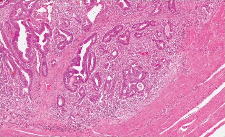
The top image of Figure 4 is a representative field of view at 0.6x magnification of an H and E stained tissue section taken from a gastrointestinal stromal tumor of the stomach that has been pretreated neoadjuvantly with imatinib. There are two nodules of viable tumor set within a sparsely cellular myxohyaline matrix. The gastric epithelium is present on the lower left side of the micrograph (see area near ‘*’) and there are two benign lymphoid aggregates (arrows). Within the tumor nodules there is histological heterogeneity. For example, the smaller nodule (a) is comprised of epithelioid cells arranged in cord-like arrays and separated by myxohyaline matrix. The larger nodule is comprised of three rather distinctive histological patterns. The upper left part of the nodule (b) consists of closely-spaced spindle cells, with oval nuclei and scant cytoplasm, with very little intervening matrix; while the lower right part (c) has a population of epithelioid and spindle cells, many with exhibiting a vacuolated cytoplasm. Along the lower right edge of the large nodule (d), the histology is similar to that seen in the smaller nodule.

Figure 4.

Histopathological description of a section of gastrointestinal stromal tumor of the stomach. The topmost image depicts a representative field of view of a gastrointestinal stromal tumor, an H and E slide of the stomach taken digitally, at 0.6x magnification. Two tumor nodules with varying morphologies are present along with two benign lymphoid aggregates (arrows). The gastric epithelium is present on the lower left portion (asterisk). The smaller nodule comprises of epithelioid cells in a cord-like arrangement and is surrounded by a myxohyaline matrix (a). The larger nodule on the left consists of three distinct tumor morphologies. The lower right border (d) has a similar appearance to that of the smaller nodule. The upper left region (b) of the larger nodule comprises of more compactly arranged spindle cells, with more hyperchromatic nuclei and a sparse hyaline matrix. The middle and middle right part (c) consists of epithelioid and spindle cells, many with vacuolated cytoplasm

To identify the optimal ring vectors that correspond to these three distinct tumor morphologies, the automated vector selection tool was used, to select them from their corresponding location within the tumor. To identify the optimal vector for region A, the GT region was selected from within the nodule on the right and multiple GN regions were chosen from the stroma, gastric epithelium, and lymphocytic aggregates [Figure 5b]. The ring vector which possessed the greatest AUC (0.987) was obtained by then searching the entire image, based upon GT and GN validation regions. Finally, a threshold map was created [Figure 5c] that accurately identified the nodule on the right, and also the lower right periphery of the larger nodule on the left, corresponding to its spatial location as described earlier.

Figure 5.

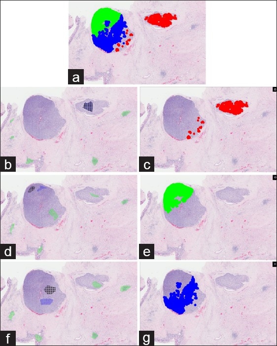
Use of three vectors to match three distinct tumor morphologies. The VSA, GN, and GT areas were selected to represent three distinct tumor morphologies seen in two tumor foci. Incidentally, the tumor morphology of the lower right border of the larger foci was similar to that of the smaller foci to the right, thus the VSA and GT areas were chosen from the smaller foci (b). A threshold map (c) was created using the vector with the highest AUC value. Similarly, the VSA, GT, and GN areas were made for the two other distinct tumor morphologies seen in the larger tumor foci (d, f), and their corresponding threshold maps are shown (e,g). The regions highlighted by the three threshold maps are combined into the topmost figure (a). Regions D and A from figure 4 were highlighted in red by one vector. Regions B and C were highlighted by two separate vectors and their matching areas are colored in green and blue, respectively.

To identify the optimal ring vector in B, the GT regions were selected from the upper left region of the big nodule on the left and the GN regions were chosen from the stroma, gastric epithelium, region A, region C and the two lymphocyte aggregates [Figure 5d]. All the ring vectors from the VSA had an AUC of 1 and their corresponding threshold map is shown in Figure 5e which corresponded to its spatial location described above.

To identify the optimal ring vector in C, the GT region was selected from the middle of the nodule, and the GN regions were selected from the stroma, gastric epithelium, region A, and the two lymphocytic aggregates [Figure 5f]. The ring vector with the greatest AUC obtained from this iterative search (AUC=0.988) was used as the basis of the threshold map depicted in [Figure 5g], which corresponded with its spatial location as described earlier.

A combination of the threshold maps demonstrated the near complete automated selection of both tumor nodules, with no spurious background features being also identified [Figure 5a]. To qualitatively compare hand-selected vectors to AVS-derived vectors, we compared the ROC curves and their associated AUCs. A ground truth map was created by painting the three unique morphologic areas of the tumor by a pathologist. Two sets of randomly hand-selected vectors were compared with the AVS-derived vector of each of the three tumor regions. In these pair-wise assessments, we identified a difference in the obtained ROC curves [Figure 6] and their respective AUCs, between the AVS-derived vector as compared to the hand-selected vectors in region A (AVS: 0.9940, hand selected #1: 0.9016, hand selected #2: 0.9827), and no significant differences in region B (AVS : 0.9912, hand selected #1: 0.9918, hand selected #2: 0.9867) and region C (AVS: 0.9915, hand selected #1: 0.9912, hand selected #2: 0.9909).

Figure 6.

ROC curve family comparing AVS to hand-selected vectors. The ROC curves were obtained from an AVS-derived and two stochastically-derived candidate vectors. The curve derived from region a/d (of Figure 4) demonstrated a better ROC curve in the case of AVS-derived vectors. The corresponding AUCs were 0.9940, 0.9016, and 0.9827 for the AVS-derived vector, hand-selected vector #1, and hand-selected vector #2, respectively.

DISCUSSION

Although the core SIVQ algorithm has general utility as an interactive, user-directed foreground feature selection tool, its utility for assisting with large-scale image analysis and image discovery studies is hampered by: (1) the single-threaded design of the originally reported reference software version and (2) the stochastic matching performance of such obtained user-selected vectors, which do not exhibit uniform sensitivity and specificity. To allow for simplified performance and surface area scaling of this algorithm, some metric of performance improvement is required for both of the above-mentioned limitations.

In this study, the former issue was addressed with linear parallelization of computational analysis, as made possible by the use of the MATLAB™ extensions module; the latter issue was addressed by spatial-numerical methods that incorporated an exhaustive search of a vector selection space against both preselected ground truth positive and negative regions, with this overall construct allowing for the identification of highly optimized vectors that exhibited theoretically maximal AUC characteristics for the areas under test. Collectively, these two functional enhancements contributed toward SIVQ now being more suitable for deployment in high-throughput discovery settings.

Soft tissue sarcomas represent one of the most heterogeneous tumor morphology classes and underscoring this reality is the fact that they have their own classification scheme based on such differences: epithelioid, pleomorphic, round cell, and spindle cell. The tumor in this study was composed of epithelioid and spindle cells + / – vacuoles. Thus, the task of identifying tumor areas from such soft tissue sarcomas would appear to be an ideal use case, owing to their morphological heterogeneity. Identifying vectors that exhibited both high sensitivity and specificity for tumor tissue were not readily attainable by manual selection. However, with the use of the VSA construct to generate optimal vectors, as already described, it became possible to greatly increase the AUC, and thus, the overall detection performance of the SIVQ analysis. Finally, using such fully-automated VSA methods, it was possible to comprehensively match the three predominant morphologies of the selected tumor, with no more than three vectors, without their matching similar-looking background features. In addition, use of the AVS technique allowed for a transition from the vector selection process of merely being a stochastic process to it being a true quantitative and rigorous selection process. Perhaps, most importantly, the availability of quantitative data, in the form of AUC figures of merit for each and every possible candidate vector, provided a previously unavailable body of quantitative data, and with it, actual statistical confirmation that the vector was indeed of high quality with regards to its matching potential (a task that was otherwise unavailable by human visual inspection of simple heatmaps).

Spatially invariant vector quantization – MATrix LABoratory

There are many advantages of working within the MATLAB™ environment. First, MATLAB™ provides a host of tools for image processing, statistical analysis, and visualization. Furthermore, MATLAB™ offers a simple, but effective means for leveraging all available processors. Specifically, by using MATLAB™, each processor can run SIVQ on a different image simultaneously. Thus, for a machine with N processors, applying SIVQ to N images requires the same time (approximately) as effecting SIVQ on a single image using the GUI. Finally, since MATLAB™ is a prevalent tool for both engineers and computer scientists. By interfacing SIVQ with MATLAB™ we have significantly increased its possible audience.

Most importantly, interfacing SIVQ to MATLAB™ allows us to leverage the considerable computing resources of the Laboratory for Computational Imaging and Bioinformatics (LCIB), at the Rutgers University. LCIB has a cluster of six high-performance Linux machines. All have eight processors and at least 32 Gigabytes of memory; the machine with the greater computation power has a Super Micro X8DTN+ motherboard with two Quad-Core Xeon X5550 (2.66 GHz) processors and 72 Gigabytes of RAM. This computer cluster provides a means for simultaneously applying SIVQ to multiple high-resolution histological images (e.g., radical prostatectomy specimens digitized at 40x).

Finally, interfacing SIVQ with MATLAB™ allows for simplified integration of the former with the robust and extensive image analysis library of the latter, facilitating the creation of additional software tools for the development, analysis, and deployment of complex image analysis algorithms, while at the same time benefiting from the performance improvement made possible by parallel computation.

In summary, we anticipate that the two described SIVQ performance enhancements of high-throughput parallel computation and automated optimal vector selection would likely be important features of future automated clinically-deployed feature selection systems that would be employed in large longitudinal clinical outcome studies, where large-scale histological assessment would be de rigueur.

Disclosure/Conflict of Interest

AM and JM are majority stockholders in Ibris Inc.

Funding

This work was made possible via grants from the Wallace H. Coulter Foundation, National Cancer Institute (Grant Nos. R01CA136535-01, R01CA140772-01, and R03CA143991-01), and the Cancer Institute of New Jersey; and at the University of Michigan by Clinical Translational Science Award (CTSA) 5ULRR02498603 PI Ken Pienta.

REFERENCES

- 1.Gray R. Vector Quantization. IEEE ASSP Magazine. 1984;1:4–29. [Google Scholar]
- 2.Linde Y, Buzo A, Gray R. An algorithm for vector quantizer design. IEEE Trans Commun. 1980;28:84–95. [Google Scholar]
- 3.Linde Y, Buzo A, Gary RM. An Algorithm for vector quantization. IEEE Trans Commun. 1980;28:84–95. [Google Scholar]
- 4.Ojala T, Pietikainen M, Maenpaa T. Multiresolution gray-scale and rotation invariant texture classification with local binary patterns. IEEE Trans Pattern Anal Mach Intell. 2002;24:971–87. [Google Scholar]
- 5.Takacs G, Chandrasekhar V, Tsai S, Chen D, Grzeszczuk R, Girod B. Unified Real-Time Tracking and Recognition with Rotation-Invariant Fast Features. Computer Vision and Pattern Recognition (CVPR), IEEE Conference on. 2010:934–41. [Google Scholar]
- 6.Hipp JD, Cheng JY, Toner M, Tompkins R, Balis U. Spatially Invariant Vector Quantization: A pattern matching algorithm for multiple classes of image subject matter including pathology. J Pathol Inform. 2011;2:13. doi: 10.4103/2153-3539.77175. [DOI] [PMC free article] [PubMed] [Google Scholar]
- 7.Hipp J, Cheng J, Hanson JC, Yan W, Taylor P, Hu N, et al. SIVQ-aided laser capture microdissection: A tool for high-throughput expression profiling. J Pathol Inform. 2011;2:19. doi: 10.4103/2153-3539.78500. [DOI] [PMC free article] [PubMed] [Google Scholar]