Robust Association Tests Under Different Genetic Models, Allowing for Binary or Quantitative Traits and Covariates

Abstract

The association of genetic variants with outcomes is usually assessed under an additive model, for example by the trend test. However, misspecification of the genetic model will lead to a reduction in power. More robust tests for association might therefore be preferred. A useful approach is to consider the maximum of the three test statistics under additive, dominant and recessive models (MAX3). The p-value however has to be adjusted to maintain the type I error rate. Previous studies and software on robust association tests have focused on binary traits without covariates. In this study we developed an analytic approach to robust association tests using MAX3, allowing for quantitative or binary traits as well as covariates. The p-values from our theoretical calculations match very well with those from a bootstrap resampling procedure. The methodology is implemented in the R package RobustSNP which is able to handle both small-scale studies and GWAS. The package and documentation are available at http://sites.google.com/site/honcheongso/software/robustsnp.

Association study is a very useful tool for revealing susceptibility variants in diseases. With the recent advances in technology, genome-wide association studies (GWAS) have been increasingly popular. The association of a genetic variant with a disease or quantitative trait is usually assessed under an additive model of inheritance. In other words, we assume that the disease risk or trait value depends upon the number of copies of the risk allele. For example, the commonly used Cochran–Armitage trend test for binary outcomes assumes an additive model (Sasieni 1997). More generally, the genotype is usually coded as 0, 1 or 2 according to the dose of the risk allele in regression models.

However, in reality it is often impossible to know the true model of inheritance beforehand. Misspecification of the genetic model leads to a reduction in power. For instance, when the recessive or dominant model is real, assuming additivity will result in power loss. More robust tests for association might therefore be preferred over model-dependent methods such as the trend test. An intuitive approach is to consider the maximum of the three test statistics under additive, dominant and recessive models (MAX3) (Freidlin et al. 2002; Gonzalez et al. 2008). Nevertheless, multiple testing needs to be taken into account to prevent inflation of type I error rate. Since the test statistics under these 3 models are not independent, a Bonferroni correction is over-conservative. Resampling-based methods, such as permutation and bootstrap, can be used to estimate the distribution of the MAX3 statistic under the null, but they are computationally expensive. In GWAS, very large numbers of markers are genotyped and we need enormous number of permutations (or runs of other resampling procedures) to achieve very low p-values.

Gonzalez et al. (2008) derived the asymptotic distribution of the likelihood ratio test statistics under H₀ for 2 × K table (K is the number of independent variables) and hence the p-value could be calculated analytically. In a similar vein, Zheng and Ng (2008) proposed the genetic model selection (GMS) test. In the first stage, the best genetic model is chosen based on a Hardy–Weinberg disequilibrium trend test between controls and cases and the chosen genetic model is tested in the second stage. The authors computed the p-value analytically by considering the proper null distribution of the GMS statistic.

The majority of previous studies on robust association tests considering different models of inheritance have focused on binary outcomes and assumed no covariates, with the exception of Li et al. (2008). In practice, other types of outcomes such as quantitative traits are often studied. Covariates are also commonly included in association studies. For instance in GWAS, researchers often correct for population stratification by including principal components (e.g. from EIGENSTRAT) (Price et al. 2006) that capture the ancestry differences in the sample. In many instances other clinical covariates (e.g. age) are also included in association studies.

Li et al. (2008) considered the Wald test and proposed estimating the covariance matrix between the 3 test statistics by solving estimating equations. The p-values for MAX3 were approximated by the “rhombus formula” that was developed based on Efron (1997). In this study, we propose and implement an alternative analytic approach to robust association tests employing MAX3, allowing for quantitative or binary outcomes as well as covariates. The approach is based on previous work by Lin (2005a), who developed a Monte-Carlo procedure to evaluate significance levels in large-scale genomic studies. We found that the concept can also be applied to robust association tests.

Our approach is based on score tests and can potentially be employed in other scenarios, as long as a score statistic can be formed. Compared to the Wald test as applied in Li et al. (2008), the score test is computationally much faster as it does not require computation of the maximum likelihood estimate (MLE) of regression coefficients. As we are usually only interested in the coefficients of the few top SNPs in a GWAS, the score test saves the time in estimating coefficients for the majority of SNPs that do not show high levels of significance. In addition, the Wald test may not be reliable in logistic regression especially when the effect size is large (or more generally when the true parameter value is far away from the null) (Hauck and Donner 1977).

Many other related tests have also been proposed. An example is the constrained likelihood ratio test (CLRT) (Wang and Sheffield 2005), which makes the restriction that the heterozygous genotype has a mean effect in between the two homozygous genotypes (i.e. no over-dominance). CLRT can deal with binary or quantitative traits and the authors have pointed out its potential to be generalized to models with covariates. The issue of covariates however was not explored in Wang and Sheffield (2005). Programs implementing CLRT have not been publicly available yet. Compared to CLRT, MAX3 might be easier to interpret and is more conceptually familiar to researchers since it is simply based on taking the maximum of the three well-known inheritance models. Also based on the assumption of no over-dominance, Yamada and Okada (2009) proposed a very similar test known as the optimal dose–effect mode trend test. Alternatively, one may also take the minimum of the p-values from the Pearson’s chi-square test and trend test. This approach (denoted MIN2) was studied by Joo et al. (2009). Simulation studies on MAX3, CLRT and MIN2 under various genetic models suggest that they have similar power (Joo et al. 2009, 2010). We shall focus on MAX3 in the current study.

Relatively few programs are available for obtaining valid p-values when testing multiple genetic models. SNPassoc (Gonzalez et al. 2007) and Rassoc (Zang et al. 2010) are two R packages that offer such options. SNPassoc includes a function (maxstat) that implements approach by Gonzalez et al. (2008). Rassoc allows the calculation of MAX3 and GMS for case–control association studies (Zang et al. 2010). However, none of the available programs allow continuous traits and none offer the option of including covariates in association tests. We have implemented our proposed methodology in a new R package called RobustSNP that is able to tackle these problems.

Methods

General theory: covariance of score functions

The theory described below followed closely the Monte-Carlo simulation approach proposed by Lin (2005a) for assessing statistical significance in multiple testing scenarios. As pointed out by Lin, all the commonly employed statistics are related to the score statistic and can be expressed as or approximated by

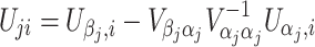
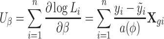
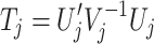where the subscript j refers to the jth hypothesis we want to test and

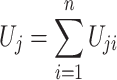where U _ji is the score function calculated from data from the ith subject only and n refers to the sample size.

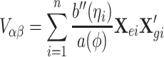
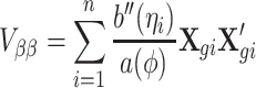
V _j is given by

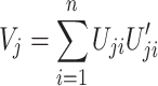When the jth hypothesis is truly null, U _j is approximately normally distributed with mean 0 and covariance matrix V _j in large samples. Hence T _j follows an approximately chi-square distribution with degrees of freedom equal to the dimension of U _j.

Consider testing a total of m hypotheses to be tested. If all of them are truly null, with large samples, (U ₁, U ₂,…,U _m) follows approximately a multivariate normal distribution with mean vector 0 and the covariance between U _j and U _k of any two hypothesis tests j and k is

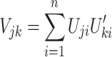This result forms the basis of our procedure to correct for the testing of multiple genetic models. In brief, we construct the score statistic for each of the three genetic models (dominant, recessive and additive) and use the above formula to calculate the covariance matrix of the three statistics under the null. The appropriate significance level is obtained by trivariate integration.

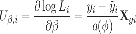
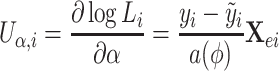
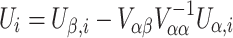
When covariates are present, U _ji in the above formulae should represent the ith subject’s efficient score function for β _j, the parameter of interest (Bickel et al. 1993; Lin 2005a, b). We have

where and are the score function for the ith subject for parameters β _j and α _j, α _j being the nuisance parameter(s). and are sub-matrices of the limiting Fisher information matrix of β _j and α _j [ equals and equals the ].

Application to genetic association studies

An example of application of score tests to genetic association studies may be found in Schaid et al. (2002). Here we shall focus on generalized linear models (GLMs) and adapt some of the work by Schaid (with modifications) in the following derivations.

For simplicity, we shall just consider a single test and the subscript j will be dropped. We are interested in testing the effect of a genetic marker under different genetic models, with or without covariates. For the ith subject, let y _i be the measured outcome, X _gi be the coding of the genotype and X _ei be a vector of environmental covariates (“environmental” here just refers to any covariates to be adjusted for) including 1 as the first element (for the intercept). X _gi is coded differently under different genetic models. Denoting the three genotypes of a markers by aa, Aa and AA, they will be coded as (0, 1, 2), (0, 1, 1) and (0, 0, 1) under additive, dominant and recessive models respectively. A is assumed to be the risk allele.

One can adjust the above coding scheme to deal with imputed genotypes. Most imputation programs produce explicit probabilities of the genotypes aa, Aa and AA. For each individual, the coding under an additive model is Pr(Aa) + 2 Pr(AA) (i.e. the standard dosage output by programs). The coding under a dominant model is Pr(Aa) + Pr(AA) while the coding under a recessive model is Pr(AA).

Assume that the outcome y and the predictor variables (X _gi, X _ei) are related through a GLM,

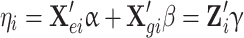where 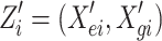and γ = (α, β). Consistent with previous notations, the parameters α and β reflect the effects of the environmental covariate and genetic marker on the outcome respectively. η is related to the actual outcome y through the link function f, such that . The likelihood of the observed outcome y _i given covariates Z _i for the ith subject is

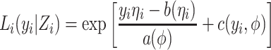where a, b and c are known functions and ϕ is the dispersion parameter.

We are interested only in testing the parameter β. The score function for genetic markers, with adjustment for environmental covariates, can be written as

Note that the score test is constructed under the null hypothesis, i.e. β = 0, hence is the fitted value when the trait is regressed on the environmental covariates only. needs to be calculated only once even when a large number of SNPs is tested.

The contribution from the ith subject is

Similarly, we have

The variance and covariance of the score functions of α and β are

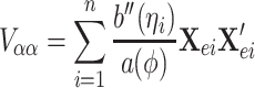Using the above results, the ith subject’s contribution to the efficient score function can be calculated by

as described previously. The forms of a(ϕ), b″(η _i) and for linear, logistic and Poisson regressions are given by Schaid et al. (2002). They are included in Table 1 for easy reference.

Table 1.

Parameters for different distributions in a GLM

Distribution		a(ϕ)	b″(η)/a(ϕ)
Binomial	exp(η)/[1 + exp(η)]	1
Normal	η		1/
Poisson	exp(η)	1

mean squared error

The efficient score functions are calculated for each subject and for each genetic model. Since each test is 1 df, we use the z-statistic in the form . Denote the z-statistic from two genetic models by Z_j and Z_k, the covariance between them is given by

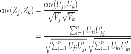Hence the covariance matrix of the z-statistics for all genetic models can be determined. Considering the case where additive, dominant and recessive models are tested. Let the observed maximum z-statistic be c and the maximum z under the complete null hypothesis be Z_null,max,

where φ ₃ is the trivariate normal distribution with covariance matrix Σ. The integral is computed by numerical methods (Genz 1992) implemented in the R package mvtnorm.

Working with the R package RobustSNP

We developed an R package RobustSNP that implements the previously described methodology. Here we briefly describe how users may perform analyses with this program. The inputs required include a file containing the outcomes (binary or quantitative) and genotypes coded as 0, 1 or 2 according to allelic counts. A file of covariates may also be included but is optional. Alternatively users can directly specify the inputs as matrices or data-frames in R.

To facilitate the analysis of GWAS, we also provide two other functions Rbin.block and Rlinear.block. These two functions accepts binary PED files from PLINK (Purcell et al. 2007) as inputs. Binary PED files are very commonly used in GWAS due to its compact size. The binary PED files are first read by the “read.plink” function in the package snpMatrix (Clayton and Leung 2007). The genotype file is then loaded in blocks (e.g. 5,000 SNPs at a time) for association analysis under different genetic models. This strategy aims to reduce the memory requirement when analyzing large-scale datasets.

The program outputs include (1) the z-statistics and p-values under additive, dominant and recessive models using the score test; (2) the p-value based on the maximum of the three genetic models, adjusted for multiple testing; (3) the error estimate from trivariate integration. The results are arranged in a tabular format with each row representing a SNP.

Results

Example application to a real dataset

To illustrate the utility of the proposed approach, we applied the methodology via RobustSNP to a real dataset of genome-wide association study on schizophrenia in a Chinese population (So et al. 2010). After quality control procedures, the dataset consisted of 473,931 SNPs from 481 cases and 2,034 controls. SNP associations with the disease were tested by logistic regression. Population stratification was corrected by including the top 10 principal components derived from EIGENSTRAT (Price et al. 2006) as covariates. Table 2 shows an excerpt of the results from chromosome 1 together with the p-values from bootstrap resampling (the bootstrap procedure is detailed below).

Table 2.

Example of robust association tests as applied to a schizophrenia dataset with 10 covariates

SNP	Z.add	Z.dom	Z.rec	P.add	P.dom	P.rec	Theoretical combined p	Bootstrap combined p	Integration error
1	0.910	−0.282	0.912	0.363	0.778	0.362	0.597	0.596	7.60E−05
2	0.424	0.482	1.034	0.672	0.630	0.301	0.500	0.509	4.32E−05
3	0.774	0.862	1.092	0.439	0.389	0.275	0.479	0.469	1.37E−04
4	1.826	−1.999	1.347	0.068	0.046	0.178	0.095	0.103	6.99E−04
5	1.888	−1.735	1.645	0.059	0.083	0.100	0.119	0.116	5.07E−04
6	0.656	−1.366	0.276	0.512	0.172	0.783	0.321	0.313	2.04E−04
7	1.023	−1.358	0.970	0.306	0.175	0.332	0.321	0.282	5.29E−04
8	1.379	−1.724	0.998	0.168	0.085	0.318	0.169	0.164	5.30E−04
9	1.242	−2.475	0.546	0.214	0.013	0.585	0.029	0.03	6.68E−04
10	2.055	−3.517	1.066	0.040	0.000437	0.286	0.001	0.002	1.38E−04
11	1.186	−1.009	0.946	0.236	0.313	0.344	0.416	0.422	4.97E−05
12	1.051	−0.756	0.955	0.293	0.450	0.340	0.497	0.481	5.69E−05
13	1.593	−0.800	1.728	0.111	0.424	0.084	0.166	0.169	1.98E−04
14	1.620	−0.741	1.885	0.105	0.459	0.059	0.120	0.098	2.74E−04
15	1.836	−1.319	1.678	0.066	0.187	0.093	0.134	0.118	2.51E−04
16	1.285	0.575	1.780	0.199	0.566	0.075	0.149	0.153	5.19E−04
17	−0.477	1.258	−0.070	0.634	0.209	0.944	0.377	0.366	2.38E−04
18	−1.575	1.742	−0.898	0.115	0.081	0.369	0.162	0.147	1.50E−04
19	−0.664	2.133	0.117	0.507	0.033	0.907	0.069	0.06	3.05E−04
20	−1.861	1.270	−1.676	0.063	0.204	0.094	0.128	0.108	4.23E−04

Z.add, Z.dom and Z.rec are the z-statistics under the additive, dominant and recessive models respectively. Similarly, P.add, P.dom and P.rec are the p-values under the three genetic models. Theoretical combined p is the p-value adjusted for multiple testing of different genetic models, obtained by the proposed analytic approach. Bootstrap combined p represents the same p-value obtained by 1,000 bootstraps. Integration error is the estimated error from computing the trivariate integral using mvtnorm

Running time

A block-size of 5,000 was used (i.e. loading 5,000 SNPs at a time). The entire analysis by RobustSNP took 17.9 h (excluding X chromosome SNPs). The time for dataset loading has already been included. The average time taken for a single SNP analysis was therefore ~0.139 s. For a comparison, we also employed PLINK to run logistic regressions on the same dataset for a single genetic model. The time taken was 5 h and 38 min. Hence the equivalent time taken for three models was ~16.9 h for PLINK. The time taken for a standard regression analysis and a robust analysis by maximizing test statistics over genetic models are in fact not very much different. In practice, one can also perform the analysis in parallel, for example by considering each chromosome at a time.

Comparing our theoretical results with bootstrap

To check the validity of our approach, we compare the p-values obtained from our theoretical calculations with a bootstrap procedure. Note that when covariates are present, a permutation approach that shuffles the phenotypes values may not be valid. As pointed out in Lin (2005a), in particular the empirical distribution generated by permutations may be invalid when covariates are correlated with both the genotype and phenotype. We therefore choose to test the validity of our proposed methodology by a bootstrap procedure. We employed the null-shift and scale-transformed bootstrap procedure as detailed in Dudoit et al. (2004) and procedure 2.3 in Dudoit and van der Laan (2007). Briefly, the cases and controls are sampled with replacement separately and the test statistics are re-calculated on each bootstrapped dataset. The test statistic are then null-centered (each test statistic subtracted from its mean in bootstrap samples) and scale-transformed as described in the references. The null-centered and scale-transformed test statistic is in the following form:

denotes the test statistic of test j from bootstrap samples of size n. Since we are testing three genetic models, j will range from 1 to 3. λ₀(j) and τ₀(j) are the known null mean and variance of the test statistic corresponding to jth test (e.g. for a z-statistic under the null, the mean is 0 and variance is 1). We performed 1,000 bootstraps for each SNP. The number of bootstraps was not further increased since the procedure is time-consuming.

We compared our theoretical p-values with bootstrap p-values on a block of 100 SNPs chosen from chromosome 1 (mimicking a fine-mapping association study). Figure 1 shows a plot of the results. It is obvious that the resampling and theoretical approaches produce very similar results. The correlation between the two sets of p-values was almost perfect (r = 0.997). We also tried to pick a random set of 300 SNPs (such that the chosen SNPs are uncorrelated) and compared the p-values under the two approaches. SNPs with only two genotypes were excluded. The plot in Fig. 2 again shows excellent correspondence of theoretical p-values with bootstrap p-values (r = 0.995). In addition, we have further picked a panel of nine random SNPs with very low p-values (p < 10⁻⁴) and investigate the concordance between the theoretical and the bootstrap p-values (using 300000 bootstraps). Table 3 showed that the p-values agreed reasonably well.

Fig. 1.

A block of 100 SNPs from a real dataset was extracted. Analytic p-values from robust association tests were plotted against the p-values obtained from a bootstrap resampling procedure. One thousand bootstraps were run for each SNP. The correlation (r) is 0.997

Fig. 2.

A random set of 300 SNPs from a real dataset were extracted. Analytic p-values from robust association tests were plotted against the p-values obtained from a bootstrap resampling procedure. One thousand bootstraps were run for each SNP. The correlation (r) is 0.995

Table 3.

Concordance between the theoretical and bootstrap results for a random panel of SNPs with low p-values

Z.add	Z.rec	Z.dom	P.add	P.rec	P.dom	Theoretical p	Bootstrap p
−4.132	2.135	4.461	3.59E−05	3.28E−02	8.14E−06	2.13E−05	2.00E−05
2.840	−4.365	1.220	4.51E−03	1.27E−05	2.23E−01	2.62E−05	3.67E−05
2.084	−4.286	1.434	3.72E−02	1.82E−05	1.52E−01	3.64E−05	1.67E−05
−3.386	1.227	−4.308	7.08E−04	2.20E−01	1.65E−05	3.80E−05	3.67E−05
4.209	−2.620	3.880	2.56E−05	8.80E−03	1.04E−04	5.10E−05	6.00E−05
1.927	−4.152	1.106	5.40E−02	3.30E−05	2.69E−01	6.60E−05	3.00E−05
4.136	−4.050	3.129	3.54E−05	5.12E−05	1.76E−03	7.03E−05	7.33E−05
1.213	−4.109	0.562	2.25E−01	3.97E−05	5.74E−01	7.95E−05	5.67E−05
3.323	−4.089	1.758	8.91E−04	4.34E−05	7.87E−02	8.50E−05	9.00E−05

Discussion

We have developed and implemented an algorithm for maximizing test statistics over different genetic models. The method was based on theories developed by Lin (2005a, b) concerning the covariance of score statistics. The asymptotic theory presented in Lin (2005a) assumes the number of hypothesis tests m is fixed and the sample size n tends to infinity. Simulations Lin (2005a) however showed that proper control of family-wise error was attained when the sample size exceeds 100 and m ranges from a few hundreds to a few thousands. For the current application, we are considering three tests (additive, dominant and recessive, i.e. m = 3) only at one time and the sample size for genetic association studies or GWAS are usually over a few hundreds and commonly more than a thousand. The number of subjects is likely to continue to rise in view of increasing collaboration between study groups. Therefore, in our case we have n ≫ m and there are no problems with the proposed analytic method.

We have not studied the power of different robust association procedures in this paper. In fact there are already numerous studies that investigated the power of various procedures such as MAX3, CLRT, MIN2 and the trend test alone (Freidlin et al. 2002; Gonzalez et al. 2008; Joo et al. 2009, 2010). Overall, the trend test performs the best when the true model is additive, but the gain in power is small compared to other robust tests (MAX3, CLRT, MIN2). Under the dominant model, all tests have comparable power. However, when the underlying model is recessive, the robust tests are more powerful than the trend test which assumes additivity. Freidlin et al. (2002) showed that employing the additive test results in substantial power loss if the true disease model is recessive, especially for alleles with low frequency (say <0.1). For instance, according to Freidlin et al. (2002), for a study with 500 cases and 500 controls and a risk allele frequency of 0.1, the power estimates of the additive, recessive and MAX3 test are 35.7, 79.4 and 71.4% respectively. If the risk allele frequency is 0.3, the power estimates of the three tests are 54, 79.5 and 72% respectively. These results suggest that recessive effects may be missed if additive models are used. The robust test MAX3 protects against model misspecification and substantially improves the power particularly for lower-frequency variants.

The three types of robust procedures MAX3, CLRT and MIN2 have similar power in general. While previous simulations were conducted without consideration of covariates, we expect that the performance of the various tests will be similar even when covariates are included. Note that for MIN2, there are yet no analytic methods for calculating the correct p-value for models with covariates, therefore resampling procedures are needed if its performance is to be investigated. Extensive simulations to test the performance of different methods in the presence of covariates may be warranted and will be a topic for further investigation.

We have focused on population-based studies in this paper. Extension to family-based studies might be of interest. The MAX3 test has been extended to TDT (Joo et al. 2010; Zheng et al. 2002), but a methodology to deal with covariates and more complex family structure has yet to be developed. Our proposed approach can potentially be applied to family-based studies if the efficient score statistics can be specified under the three inheritance models.

Two-stage designs are also very common for GWAS and how to take into account of uncertain genetic model in this setting is another interesting topic. In a two-stage design, a set of the most significant SNPs are chosen from the 1st stage and replication was performed at the 2nd stage. Kwak et al. (2009) proposed a robust procedure performing GMS in this scenario, however quantitative traits and covariates have not been considered. Further work is required to extend Kwak et al’s procedure to deal with more diverse models.

Another question is how to combine the results across different studies in meta-analyses. Typically the inputs for meta-analysis are summary test statistics rather than the raw data. For a study that includes covariates, one cannot perform the MAX3 test based on summary statistics alone. However, if robust tests have been performed for each individual study, then one may directly combine the p-values, for example by the Fisher’s method.

In conclusion, we have developed an algorithm and an R package RobustSNP for obtaining valid p-values for robust association testing of different genetic models. The algorithm avoids the need for resampling procedures which are computationally expensive. Compared to other studies (or software packages) that focus on robust association tests, the method presented here allows for both quantitative and binary outcomes and is able to deal with covariates. We believe the method and program presented here will be useful to genetic researchers and will help to uncover susceptibility variants that may otherwise be missed by standard analysis assuming additive models only.

References

- Bickel PJ, Klassen CAJ, Ritov Y, Wellner JA. Efficient and adaptive estimation in semiparametric models. Baltimore: The Johns Hopkins University Press; 1993. [Google Scholar]
- Clayton D, Leung HT. An R package for analysis of whole-genome association studies. Hum Hered. 2007;64(1):45–51. doi: 10.1159/000101422. [DOI] [PubMed] [Google Scholar]
- Dudoit S, van der Laan MJ. Multiple testing procedures and applications to genomics. New York: Springer; 2007. [Google Scholar]
- Dudoit S, van der Laan MJ, Pollard KS (2004) Multiple testing. Part I. Single-step procedures for control of general type I error rates. Stat Appl Genet Mol Biol 3:Article 13 [DOI] [PubMed]
- Efron B. The length heuristic for simultaneous hypothesis tests. Biometrika. 1997;84(1):143–157. doi: 10.1093/biomet/84.1.143. [DOI] [Google Scholar]
- Freidlin B, Zheng G, Li Z, Gastwirth JL. Trend tests for case–control studies of genetic markers: power, sample size and robustness. Hum Hered. 2002;53(3):146–152. doi: 10.1159/000064976. [DOI] [PubMed] [Google Scholar]
- Genz A. Numerical computation of multivariate normal probabilities. J Comput Graph Stat. 1992;1(2):141–149. doi: 10.2307/1390838. [DOI] [Google Scholar]
- Gonzalez JR, Armengol L, Sole X, Guino E, Mercader JM, Estivill X, Moreno V. SNPassoc: an R package to perform whole genome association studies. Bioinformatics. 2007;23(5):644–645. doi: 10.1093/bioinformatics/btm025. [DOI] [PubMed] [Google Scholar]
- Gonzalez JR, Carrasco JL, Dudbridge F, Armengol L, Estivill X, Moreno V. Maximizing association statistics over genetic models. Genet Epidemiol. 2008;32(3):246–254. doi: 10.1002/gepi.20299. [DOI] [PubMed] [Google Scholar]
- Hauck W, Jr, Donner A. Wald’s test as applied to hypotheses in logit analysis. J Am Stat Assoc. 1977;72(360):851–853. doi: 10.2307/2286473. [DOI] [Google Scholar]
- Joo J, Kwak M, Ahn K, Zheng G. A robust genome-wide scan statistic of the Wellcome Trust Case–Control Consortium. Biometrics. 2009;65(4):1115–1122. doi: 10.1111/j.1541-0420.2009.01185.x. [DOI] [PubMed] [Google Scholar]
- Joo J, Kwak M, Chen Z, Zheng G. Efficiency robust statistics for genetic linkage and association studies under genetic model uncertainty. Stat Med. 2010;29(1):158–180. doi: 10.1002/sim.3759. [DOI] [PubMed] [Google Scholar]
- Kwak M, Joo J, Zheng G. A robust test for two-stage design in genome-wide association studies. Biometrics. 2009;65(4):1288–1295. doi: 10.1111/j.1541-0420.2008.01187.x. [DOI] [PubMed] [Google Scholar]
- Li Q, Zheng G, Li Z, Yu K. Efficient approximation of P-value of the maximum of correlated tests, with applications to genome-wide association studies. Ann Hum Genet. 2008;72(Pt 3):397–406. doi: 10.1111/j.1469-1809.2008.00437.x. [DOI] [PubMed] [Google Scholar]
- Lin DY. An efficient Monte Carlo approach to assessing statistical significance in genomic studies. Bioinformatics. 2005;21(6):781–787. doi: 10.1093/bioinformatics/bti053. [DOI] [PubMed] [Google Scholar]
- Lin DY. On rapid stimulation of P values in association studies. Am J Hum Genet. 2005;77(3):513–514. doi: 10.1086/432817. [DOI] [PMC free article] [PubMed] [Google Scholar]
- Price AL, Patterson NJ, Plenge RM, Weinblatt ME, Shadick NA, Reich D. Principal components analysis corrects for stratification in genome-wide association studies. Nat Genet. 2006;38(8):904–909. doi: 10.1038/ng1847. [DOI] [PubMed] [Google Scholar]
- Purcell S, Neale B, Todd-Brown K, Thomas L, Ferreira MA, Bender D, Maller J, Sklar P, de Bakker PI, Daly MJ, Sham PC. PLINK: a tool set for whole-genome association and population-based linkage analyses. Am J Hum Genet. 2007;81(3):559–575. doi: 10.1086/519795. [DOI] [PMC free article] [PubMed] [Google Scholar]
- Sasieni PD. From genotypes to genes: doubling the sample size. Biometrics. 1997;53(4):1253–1261. doi: 10.2307/2533494. [DOI] [PubMed] [Google Scholar]
- Schaid DJ, Rowland CM, Tines DE, Jacobson RM, Poland GA. Score tests for association between traits and haplotypes when linkage phase is ambiguous. Am J Hum Genet. 2002;70(2):425–434. doi: 10.1086/338688. [DOI] [PMC free article] [PubMed] [Google Scholar]
- So HC, Li M, Chen RY, Cheung EF, Chen EY, Cherny SS, Li T, Sham PC. Genome-wide association study of schizophrenia in a Chinese population. Int J Neuropsychopharmacol. 2010;13(Supplement S1):171. [Google Scholar]
- Wang K, Sheffield VC. A constrained-likelihood approach to marker-trait association studies. Am J Hum Genet. 2005;77(5):768–780. doi: 10.1086/497434. [DOI] [PMC free article] [PubMed] [Google Scholar]
- Yamada R, Okada Y. An optimal dose-effect mode trend test for SNP genotype tables. Genet Epidemiol. 2009;33(2):114–127. doi: 10.1002/gepi.20362. [DOI] [PubMed] [Google Scholar]
- Zang Y, Fung WK, Zheng G. Simple algorithms to calculate asymptotic null distributions of robust tests in case–control genetic association studies in R. J Stat Softw. 2010;33(8):1–24. [Google Scholar]
- Zheng G, Freidlin B, Gastwirth JL. Robust TDT-type candidate–gene association tests. Ann Hum Genet. 2002;66(Pt 2):145–155. doi: 10.1046/j.1469-1809.2002.00104.x. [DOI] [PubMed] [Google Scholar]
- Zheng G, Ng HK. Genetic model selection in two-phase analysis for case-control association studies. Biostatistics. 2008;9(3):391–399. doi: 10.1093/biostatistics/kxm039. [DOI] [PMC free article] [PubMed] [Google Scholar]