Automated Macular Pathology Diagnosis in Retinal OCT Images Using Multi-Scale Spatial Pyramid and Local Binary Patterns in Texture and Shape Encoding

Abstract

We address a novel problem domain in the analysis of optical coherence tomography (OCT) images: the diagnosis of multiple macular pathologies in retinal OCT images. The goal is to identify the presence of normal macula and each of three types of macular pathologies, namely, macular edema, macular hole, and age-related macular degeneration, in the OCT slice centered at the fovea. We use a machine learning approach based on global image descriptors formed from a multi-scale spatial pyramid. Our local features are dimension-reduced Local Binary Pattern histograms, which are capable of encoding texture and shape information in retinal OCT images and their edge maps, respectively. Our representation operates at multiple spatial scales and granularities, leading to robust performance. We use 2-class Support Vector Machine classifiers to identify the presence of normal macula and each of the three pathologies. To further discriminate sub-types within a pathology, we also build a classifier to differentiate full-thickness holes from pseudo-holes within the macular hole category. We conduct extensive experiments on a large dataset of 326 OCT scans from 136 subjects. The results show that the proposed method is very effective (all AUC > 0.93).

1. Introduction

Optical Coherence Tomography (OCT) is a non-contact, non-invasive 3-D imaging technique which performs optical sectioning at microscopic resolution (∼5um). It was commercially introduced to ophthalmology in 1996 (Schuman et al., 1996), and has been widely adopted as the standard clinical care in ophthalmology for identifying the presence of various ocular pathologies and their progression (Schuman et al., 2004). This technology measures the optical back scattering of the tissues, making it possible to visualize the intraocular structures, such as the retina and the optic nerve head. An example 3D ocular OCT scan is given in Fig. 1a. The ability to visualize the internal structures of the retina (the z-axis direction in Fig. 1a) makes it possible to diagnose diseases, such as glaucoma and macular hole, objectively and quantitatively.

Figure 1.

(a) Example 3D macular OCT scan (x: horizontal, y: vertical, z:depth direction) without eye motions. (b) Left: example 2D OCT en-face image (also called OCT fundus image) generated by projecting a 3D macular OCT image along z-axis to x-y plane. Middle: horizontal cross-sectional image corresponding to the red-line on the en-face image. Right: vertical cross-sectional image corresponding to the blue-line on the en-face image; significant z-directional eye motions (yellow arrows) can be observed here, which corrupt the spatial integrity of the 3D data. In the ideal motion-free case, this image shall look similar to a rotated version of the middle image.

Although OCT imaging technology continues to evolve, the development of technology to assist in the interpretation of OCT images has not kept pace. With OCT data being generated in increasingly larger amounts and captured at increasingly higher sampling rates, there is a strong need for computer assisted analysis to support disease diagnosis. This need is amplified by the fact that an ophthalmologist making a diagnosis under standard clinical conditions does not have the assistance of a specialist in interpreting OCT data. This is in contrast to other medical imaging situations, where a radiologist is usually available.

There have been some previous works addressing topics in ocular OCT image processing, such as intra-retinal layer segmentation (Garvin et al., 2008) (Ishikawa et al., 2005), optic disc segmentation (Lee et al., 2010), detection of fluid-filled areas (Quellec et al., 2010), and local quality assessment (Barnum et al., 2008). However, to our knowledge, there has been no prior work on automated macular pathology identification in OCT images. Our goal is to determine the probability that each common type of pathology is present in a given macular cross-section from a known anatomical position. Such an automated tool would improve the efficiency of OCT-based analysis in daily clinical practice, both for online diagnostic reference and for offline slice tagging and retrieval.

The macula is located at the center of the retina and is responsible for highly-sensitive, accurate vision. Acute maculopathy can cause the loss of central, sharp vision and even lead to blindness. For example, diabetic retinopathy, one of the leading causes of blindness worldwide, is often associated with macular edema (ME). According to a study conducted in 2004 (The Eye Diseases Research Prevalence Research Group, 2004), among an estimated 10.2 million U.S. adults aged 40 and older known to have diabetes mellitus, the estimated prevalence rate for retinopathy was 40.3%. Another type of maculopathy, called age-related macular degeneration (AMD), is the leading cause of visual loss among elderly persons. The Beaver Dam Eye Study reported that 30% of individuals aged 75 and older have some form of AMD (Age-Related Eye Disease Study Research Group, 2001). Another disease that can lead to blindness is called macular hole (MH), which is less common than ME and AMD. The overall prevalence is approximately 3.3 cases in 1000 in those persons older than 55 years (Luckie and Heriot, 1995). As the size of the elderly population increases in the U.S. and many developed countries, the prevalence of maculopathy has increasingly significant social and economic impact. Thus, the diagnosis and screening of macular disease is important to public health.

Our approach to automated pathology identification is based on the analysis of 2D slices from the macular OCT volume. Example slices for pathological and normal macula are shown in Fig. 2. There are two motivations for our choice of 2D slice-based analysis. The first motivation is that slice-based analysis is consistent with existing clinical practice in ophthalmology. Clinicians routinely examine the OCT volume in a slice-by-slice manner, for example by using the en-face view illustrated in Fig. 1(b)(left) as a guide for selecting and viewing slices. Thus the ability to analyze and display information about pathologies in a slice-based manner is aligned with existing practices.

Figure 2.

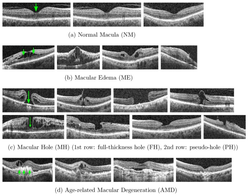
Characteristics of (a) normal macula (NM): a smooth depression shows at the center (fovea), (b) macular edema (ME) : retinal thickening and liquid accumulation appears as black blobs around the fovea, (c) macular hole (MH): a full-thickness hole (FH, 1st row) or pseudo hole (PH, 2nd row) formation at the fovea; for PH, the hole formation does not reach the outer most retinal layer (retinal pigment epitherium, RPE), (d) age-related macular degeneration (AMD): irregular contours usually extrude in dome shapes appear at the bottom layer (RPE) of the retina.

The second motivation for slice-based analysis is that the 3D OCT data itself is naturally organized as a series of slices corresponding to a sequence of x-z scans. Within each slice, the OCT data is very consistent, as shown in Fig. 1(b)(middle). However, a modern scanner such as Cirrus HD-OCT can require 2 seconds to image a target cube. During this period, misalignment across slices can occur due to the natural and involuntary movement of the subject's eyes. Involuntary movements include micro-saccade, ocular tremor and drifting (Xu et al., 2010), resulting in oscillations of up to 15 Hz. These motion artifacts are illustrated in Fig. 1(b)(right) for a 2D slice that cuts across multiple horizontal scans. These inter-slice distortions and misalignments are a significant barrier to a full 3D analysis of the OCT volume, and addressing them is a research project in its own right.

There have been a few works on eye motion correction in 3D-OCT scans (Ricco et al., 2009)(Xu et al., 2010). However, these prior works only demon-strated the correction results for optic-disc scans where the blood vessel structures act as important characteristics for feature alignment. In contrast, the macula has no obvious vessel structures and can exhibit substantial variability in appearance due to pathologies. As a consequence, these techniques may not be readily adapted to macular OCT scans. In the absence of a reliable motion correction technique for the macula data, we adopt a 2D slice-based approach.

In this paper,¹ we present our method for automatically identifying macular pathologies in a given x-z slice at a known anatomical position. Specifically, we focus on identifying the presence of the normal macula (NM) and each of the following macular pathologies, ME, MH,² and AMD, when given a x-z slice centered at the fovea³ (macula center). Fig. 2 gives example images and the appearance description for each pathology. Note that multiple pathologies can coexist in one eye, as depicted in Fig. 3a, 3b; in this case, the automated method should report the existence of both pathologies.

Figure 3.

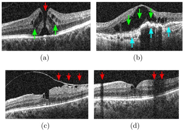
Example x-z (horizontal) slice with (a) MH (red) and ME (green), (b) ME (green) and AMD (blue), (c) a detached tissue, (d) shadowing effects.

The proposed approach can also be used to differentiate sub-categories within a pathology. For instance, our MH category contains both full-thickness holes (FH) (Fig. 2c, 1st row) and pseudo-holes (PH) (Fig. 2c, 2nd row). This distinction is clinically relevant, as these two cases are treated differently. In Section 3.6, we demonstrate the ability to discriminate these two subtypes within the MH category.

To summarize, we make two main contributions:

• The first work on automated macular pathology diagnosis in retinal OCT images.

• The development of a novel and effective image descriptor for encoding OCT slices in automated diagnosis.

The paper is organized as follows. In Section 2, we provide the rationale in designing our approach and describe each step in detail. In Section 3, we present the dataset, the definition of ground truth, and extensive experiments to validate each component of our method. Finally, Section 4 concludes this paper with discussions and future work.

2. Approach

Automated pathology identification in ocular OCT images is complicated by four factors. First, the co-existence of multiple pathologies (see Fig. 3a, 3b) or other pathological changes (e.g., detached membrane, see Fig. 3c) can confound the overall appearance, making it hard to model each pathology separately. Second, there is high variability in shape, size, and magnitude within the same pathology. In MH, for examples, the holes can have different widths, depths, and shapes, and some can even be covered by incompletely detached tissues (the 4th example in Fig. 2c), making explicit pathology modeling difficult. Third, the measurement of reflectivity of the retina is affected by the optical properties of the overlying tissues (Schuman et al., 2004), e.g., blood vessels will absorb much of the transmitted light and opaque media will block the light, and thus produce shadowing effects (Fig. 3d). Fourth, a portion of the image may have lower quality due to imperfect imaging (Barnum et al., 2008). As a result of the above factors, attempting to hand-craft a set of features or rules to identify each pathology separately is unlikely to succeed. Instead, we propose to use machine learning techniques to automatically discover discriminative features from a set of training examples.

Our analysis approach consists of three steps, which are illustrated in Fig. 4. First, image alignment is performed to reduce the appearance variation across scans. Second, we construct a global descriptor for the aligned image and its corresponding edge map by computing spatially-distributed multi-scale texture and shape features. Multi-scale spatial pyramid (MSSP) is used to encode the global spatial organization of the retina. To encode each spatial block in MSSP, we employ dimension-reduced Local Binary Pattern (LBP) histogram (Ojala et al., 2002) to capture the texture and shape characteristics of the retinal image. This feature descriptor can preserve the geometry as well as textures and shapes of the retinal image at multiple scales and spatial granularities. The last step is to train a 2-class non-linear Support Vector Machine (SVM) (Chang and Lin, 2001) for each pathology. We now describe each step in more detail.

Figure 4.

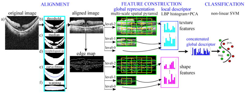
Stages of our approach.

2.1. Retina Alignment

Imaged retinas have large variations in their inclination angles, positions, and natural curvatures across scans, as shown in Fig. 2. It is therefore desirable to roughly align the retinas to reduce these variations before constructing the feature representation. To this end, we use a simple heuristic procedure to flatten the curvature and center the retina: (1) threshold the original image (Fig. 4, a) to detect most of the retina structures (Fig. 4, b); (2) apply a median filter to remove noise and thin detached tissues (Fig. 4, c); (3) find the entire retina by using morphological closing and then opening; by closing, we fill-up black blobs (e.g. cystoid edema) inside the retina, and by opening, we remove thin or small objects outside the retina (Fig. 4, d); (4) fit the found retina area with a second-order polynomial using least-square curve fitting (Fig. 4, e); we choose a low order polynomial to avoid overfitting, and thus preserve important shape changes caused by pathologies; (5) warp the entire retina to be approximately horizontal by translating each image column a distance according to the fitted curve (Fig. 4, f) (after the warping, the fitted curve will become a horizontal line); then, crop the warped retina in the z-direction with a reserved margin (see aligned result in Fig. 4). The exact parameter values used in our procedure are presented in Section 3.2.

Note that our procedure fits and warps the entire retina rather than segmenting a particular retinal layer first (e.g. the RPE layer) and then performing flattening using that layer (Quellec et al., 2010). Our approach is motivated by the fact that the state of the art methods for layer segmentation are unreliable for scans with pathologies (Ishikawa et al., 2009). In the next section, we describe an approach to spatially-redundant feature encoding which provides robustness against any remaining variability in the aligned scans.

2.2. Multi-Scale Spatial Pyramid (MSSP)

There are three motivations for our choice of a global spatially-distributed feature representation for OCT imagery based on MSSP. First, pathologies are often localized to specific retinal areas, making it important to encode spatial location. Second, the context provided by the overall appearance of the retina is important for correct interpretation; e.g., in Fig. 3d, we can distinguish between a shadow and a macular hole more effectively given the context of the entire slice. Third, pathologies can exhibit discriminating characteristics at both small and large scales; therefore, both micro-patterns and macro-patterns should be represented. For these reasons, we use a global multi-scale image representation which preserves spatial organization.

We propose to use the multi-scale version of spatial pyramid (SP) (Lazebnik et al., 2006), denoted as MSSP, to capture the geometry of the aligned retina at multiple scales and spatial resolutions. This global framework, MSSP, was recently proposed in (Wu and Rehg, 2008), where it was successfully applied to challenging scene classification tasks. Fig. 5 illustrates the differences between a 3-level MSSP and a 3-level SP. To form a k-level MSSP, for each level l (0 ≤ l ≤ (k−1)), we rescale the original image by 2^l−k+1 using bilinear interpolation, and divide the rescaled image into 2^l blocks in both image dimensions. The local features computed from all spatial blocks are concatenated in a predefined order to form an overall global descriptor, as illustrated in Fig. 4. Note that we also add the features from the overlapped blocks (the green blocks in Fig. 5) to reduce boundary effects.

Figure 5.

Structures of a 3-level MSSP and SP. The green lines indicate the overlapped blocks which can also be added in the global representation.

2.3. Histogram of LBP and Dimensionality Reduction using PCA

Local binary pattern (LBP) (Ojala et al., 2002) is a non-parametric kernel which summarizes the local structure around a pixel. LBP is known to be highly discriminative and has been successfully applied to computer vision tasks, such as texture classification (Ojala et al., 2002), face recognition (Ahonen et al., 2006), and scene classification (Wu and Rehg, 2008). It has also been effective in medical image analysis, such as texture classification in lung CT images (Sørensen et al., 2008), and false positive reduction in mammographic mass detection (Oliver et al., 2007).

While there are several types of LBP, we follow (Ahonen et al., 2006; Oliver et al., 2007; Sørensen et al., 2008) in adopting LBP_8,1 to capture the micro-patterns that reside in each local block. The LBP_8,1 operator derives an 8 bit binary code by comparing the center pixel to each of its 8 nearest neighbors in a 3×3 neighborhood, while “1” represents radius 1 when sampling the neighbors. The resulting 8 bits are concatenated circularly to form an LBP code in the range [0 255]. The computation is illustrated in Fig. 6a. The formal equation can be written as:

Figure 6.

Examples of (a) LBP_8,1 code computation, (b) uniform LBP (≤ 2 bitwise transitions) versus non-uniform LBP (> 2 bitwise transitions).

$$LB{P}_{8,1}=\sum _{n=0}^{7}f({\upsilon }_n-{\upsilon }_c)2^n$$

where f(x) = 1 if x ≥ 0, otherwise f(x) = 0; υ_c and υ_n represent the pixel value at the center and the neighboring pixel, respectively, with each neighbor being indexed circularly.

For each block of pixels in the MSSP, we compute the histogram of LBP codes to encode the statistical distribution of different micro-patterns, such as spots, edges, corners, and flat areas. Histogram descriptors have proven to be effective at aggregating local intensity patterns into global discriminative features. In particular, they avoid the need to precisely localize discriminating image structures, which is difficult in complex and highly variable OCT images. Since we compute LBP histogram in multi-scale image blocks, the distribution of both micro-patterns and macro-patterns can be encoded. Note that many previous works applied LBP only in the original image (Ahonen et al., 2006; Oliver et al., 2007; Sørensen et al., 2008), which may not capture large-scale patterns effectively.

Although a single LBP_8,1 histogram has only 256 bins, the concatenation of histograms from each block to form the global feature vector results in an impractically high dimension. We adopt PCA to reduce the dimension of LBP histogram, as proposed in (Wu and Rehg, 2008). We denote it as $LB{P}_{8,1}^{\mathit{pca}}$.

It is important to note that previous works (Ahonen et al., 2006; Oliver et al., 2007) employing LBP histogram features have adopted an alternative approach to dimensionality reduction, called uniform LBP (Ojala et al., 2002), which we have found to be less effective than $LB{P}_{8,1}^{\mathit{pca}}$. An LBP pattern is called uniform if it contains at most two bitwise transitions, as shown in Fig. 6b. A histogram of $LB{P}_{8,1}^{u2}$ is formed by retaining occurrences of each of 58 uniform patterns and putting all occurrences of 198 non-uniform patterns, denoted as $LB{P}_{8,1}^{\neg u2}$ to a single bin, resulting in 59 bins in total. It was observed by Ojala (Ojala et al., 2002) that $LB{P}_{8,1}^{u2}$ occupied 90% of all LBP_8,1 patterns in pixel count, when computed from image textures. However, as recently noted by Liao (Liao et al., 2007), when LBP codes are computed in the rescaled images, $LB{P}_{8,1}^{u2}$ may no longer be in the majority. More importantly, the distribution of individual $LB{P}_{8,1}^{\neg u2}$ patterns can contain important distinctive information for category discrimination, in spite of its low frequency of occurrences (see Fig. 7).

Figure 7.

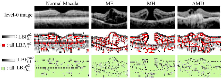
Visualization of $LB{P}_{8,1}^{u2}$ and $LB{P}_{8,1}^{\neg u2}$ on example level-0 images. All $LB{P}_{8,1}^{\neg u2}$ are shown in red in the 2nd row, and the individual $LB{P}_{8,1}^{\neg u2}$ codes are shown in gray-level in the 3rd row. We find that although $LB{P}_{8,1}^{\neg u2}$ patterns have low counts, most of them reside in the important contours and can therefore be useful for discrimination.

In Section 3 we demonstrate the superior performance of $LB{P}_{8,1}^{\mathit{pca}}$ in comparison to other LBP-based features.

2.4. Encoding Texture and Shape Characteristics

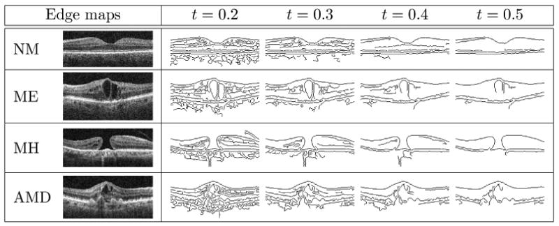
In the previous section, we have described how we use $LB{P}_{8,1}^{\mathit{pca}}$ to encode the texture property of the aligned image. It is also desirable to capture the shape characteristics of the retinal image in conjunction with the textures so that different properties are represented in our descriptor. To encode the shape characteristics,⁴ we first generate the Canny edge map (Canny, 1986) from the aligned retinal image, and then compute $LB{P}_{8,1}^{\mathit{pca}}$ for each spatial block in the MSSP representation of the edge map, as illustrated in Fig. 4. Example Canny edge maps for each pathology are shown in Table 1. Since edge maps generated from varied edge detection thresholds are different in edge quantity, in Section 3.5, we will test a variety of edge detection thresholds and report the best settings. Note that while LBP histogram has been utilized before in the medical domain to encode texture information, to our knowledge, it has not been previously applied on to shape properties.

Table 1.

Aligned images and their Canny edge maps derived by using varied edge detection thresholds t.

From the edge maps in Table 1, we observe that when t ≥ 0.3 most spurious details are suppressed, while the high-contrast boundaries become prominent. In fact, a skilled observer can identify some pathologies just from the edge map. In MH, for example, a hole contour can clearly be seen around threshold 0.4. Thus, it is possible that utilizing the shape features alone is sufficient for some categories. In Section 3.5, we will examine the effect of using texture or shape features alone, or in combination, in order to identify which feature type is more discriminative for a specific pathology.

We also would like to emphasize the power of LBP histograms in preserving the contents of a binary image, such as an edge map or a silhouette image. Wu and Rehg (2011) conducted an interesting experiment to show how LBP histogram can preserve image structures: when given the LBP histogram of a small binary image (e.g. 10×10) and a random shuffled version of this image as the input state, it is highly probable to restore the original image or a very similar one through an optimization process based on histogram matching. This reconstruction ability cannot be easily achieved if the input histogram is the intensity or orientation histogram, since more pixel arrangements can map to the same histograms. Their experiment provides strong evidence that LBP histograms can preserve the structures in a binary image.

2.5. Classification Using Support Vector Machine (SVM)

After computing the global descriptors, we train a 2-class non-linear SVM with RBF kernel and probabilistic output (Chang and Lin, 2001) for each pathology using a 1 vs. the rest approach. The kernel parameter and error penalty weight of SVMs are chosen by cross validation on the training set. The probability scores from each pathology classifier are compared to a set of decision thresholds to determine the corresponding sensitivity and specificity.

3. Experimental Results

This section is organized as follows. In Sections 3.1 and 3.2, we describe the dataset, the labeling agreement among the three ophthalmologists, the ground truth definition, and the experimental setting. In Sections 3.3 and 3.4, we validate $LB{P}_{8,1}^{\mathit{pca}}$ and MSSP by comparing them to other popular local descriptors and global frameworks, respectively. In Section 3.5 the performance of utilizing texture or shape features, both alone and in combination, are evaluated. In Section 3.6 we evaluate the ability of our method to identify subtypes in MH. Finally, in Section 3.7, we conduct a feature weight visualization experiment to show the spatial distribution of the most discriminative features.

3.1. Inter-Operator Agreement and Ground Truth

We collected 326 macular spectral-domain OCT scans (Cirrus HD-OCT; Carl Zeiss Meditec) from 136 subjects (193 eyes). The original resolution of the scans was either 200×200×1024 or 512×128×1024 in 6×6×2 mm volume (width(x), height(y) and depth(z)). All horizontal cross-section images (x-z slice) were rescaled to 200×200 to smooth out noise while retaining sufficient details for pathology identification. One image example is shown in Fig. 4 (a). For each of the 326 scans, the x-z slice crossing through the foveal center was then selected by an expert ophthalmologist.

Three OCT experts then independently identified the presence or absence of normal macula and each of ME, MH, and AMD in the fovea-centered slice. Note that multiple pathologies can coexist in one slice. The labeling agreement among the three experts is illustrated in Fig. 8 using the Venn diagram. The complete agreement among the experts for NM, ME, MH, and AMD is 96.9%, 80.1%, 91.1%, and 87.1%, respectively, where a lower agreement is observed for ME and AMD. The majority opinion of the three experts' labeling was computed separately for each pathology and used as the ground truth.⁵ The number of positive images for each pathology category as defined by the ground truth is listed in Table 2. Here, for a specific pathology, an eye/subject that has at least one positive scan is counted as positive. In Table 3, we list the scan statistics for each combination of the three pathologies. It shows that ME often co-occurs with MH or AMD.

Figure 8.

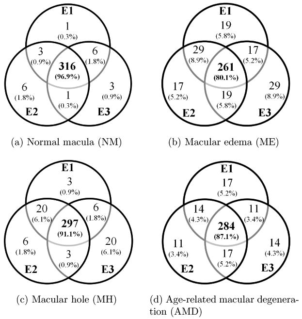
Venn diagram of labeling agreement among the three experts on all macular pathologies. The actual scan numbers and the percentages are both shown. E1-E3 represents experts 1 to 3.

Table 2.

Number of positive scans, eyes and subjects, as defined by the majority opinion of the three experts. Note that each scan was labeled with all coinciding macular findings.

Statistics	NM	MH	ME	AMD
Scan	81	74	203	74
Eye	66	36	116	37
Subject	65	33	90	26

Table 3.

Number of positive scans, eyes and subjects as defined by the majority opinion for each combination of three pathologies. For example, “MH” column represents statistics of scans with only MH, but no ME and AMD. In our dataset, there are no scans containing all three pathologies, although it is possible.

Statistics	Single Pathology Only			Combination of Pathologies
	ME	MH	AMD	ME+MH	ME+AMD
Scan	93	9	29	65	45
Eye	65	3	15	34	25
Subject	53	3	13	32	19

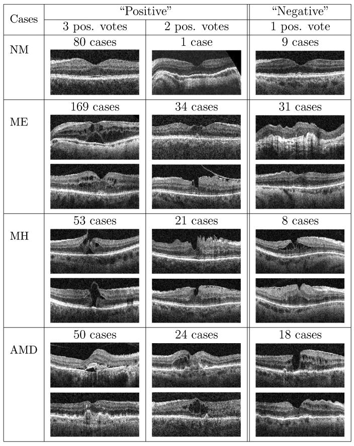
In order to further assess how many positive/negative cases result from inconsistent labeling, in Table 4, the statistics and several representative examples are shown for each pathology, where all three experts, only two experts, or just one expert gives “positive” label. Note that the images labeled as positive by only one expert were treated as negative instances in our ground truth. It was found that the quantity of images having one positive vote is considerably larger for ME and AMD (31 and 18 cases, respectively), revealing greater ambiguity in their identification.

Table 4.

The number of cases and corresponding examples where all 3 experts, 2 experts, or only one expert gives positive label for the normal macula and each pathology, respectively. Images with at least two positive votes were defined as positive while the ones with just one positive vote were regarded as negative in our ground truth. The images without complete agreements usually contain early pathologies which occupied small areas.

3.2. Experimental Setting

For the alignment preprocessing step, we used intensity threshold 60, 5×5 median filter, disk-shaped structure element with size 30 for morphological closing and size 5 for opening, and 15 pixel reserved margin at both top and bottom when cropping the retinal area in z-direction. We observed that this setting can roughly remove the curvature and center the retina area in all images in the dataset.

We use 10-fold cross validation at the subject level, where for each fold 10% of positive and negative subjects are put in the test set. All images from the same subject are put together in either the training or test set. We do not separate images from left eyes or right eyes but train and test them together. In order to further enrich our training set, both the training image and its horizontal flip are used as the training instances. The 10-fold testing results are aggregated⁶ and the area under the receiver operator characteristic curve (AUC) is computed. Note that although some subjects/eyes contribute more than one scan in our image library, these scans were taken on different dates and usually showed pathological progression or additional pathologies. Therefore, we treat each scan as a different instance, and report the AUC result at the scan level.⁷ To get a more reliable assessment of the performance, we repeat the 10-fold data splitting procedure six times, where each time a different data splitting is generated randomly, and compute the mean and standard deviation of the 6 AUCs as the performance metric.

To test the statistical significance of the performance difference between different algorithmic settings, we adopt the DeLong test (DeLong et al., 1988) to compare their receiver operating characteristic (ROC) curves. The DeLong test is widely used in biomedical research. It takes into account the correlation of the diagnostic results from different algorithms for the same test units, and can generate an estimated covariance matrix of algorithm performance, which can be used for statistical testing. We apply the test in the following way: if, under the DeLong test, one setting is found to be superior to than another at p = 0.05 significant level for all 6 different data-splitting procedures, then the performance of the best setting is claimed to be significant.

3.3. Validation of Dimension-reduced Local Binary Patterns as Local Descriptors

To validate the use of dimension-reduced LBP histograms as local features, we encode the texture properties of the aligned retinal image, and compare the resulting performance to several other popular descriptors, including mean and standard deviation of intensity (MS), intensity histogram (I), and orientation histogram (O). Each feature type is employed with a 3-level MSSP with overlapped blocks.⁸ The orientation histogram (Freeman and Roth, 1994) is formed from the gradient direction and magnitude computed from 2×2 neighborhoods. For I and O features, we use the quantization of 32 bins in intensity and angle, respectively, since this produces the best results. For LBP histograms, we quantize the intensity image to 32 levels before LBP encoding in order to suppress pixel noise; this quantization improves the accuracy of LBP by about 0.7% on average. For $LB{P}_{8,1}^{\mathit{pca}}$ computation, the principle axes are derived from the training images of each fold separately.

In feature computation, for NM, ME, and AMD, we compute the highest level features (the 2nd-level in MSSP) from the aligned image directly; for MH, these features are encoded from the further rescaled image (half size in width and height) instead. This rescaling for MH results in better performance for all descriptors (1%∼5% improvement). This can be attributed to the macro-scale nature of holes, where details present in the original resolution are not required for identification.

The AUC results are listed in Table 5 and the significance test results between $LB{P}_{8,1}^{\mathit{pca}}$ (59) and other descriptors are shown in Table 6. Overall, $LB{P}_{8,1}^{\mathit{pca}}$ (59) achieves the best average performance, $LB{P}_{8,1}^{\mathit{pca}}$ (32) is the second best, and $LB{P}_{8,1}^{u2}$ (59) is the third. For NM, ME, and AMD, most popular descriptors can achieve >0.90 AUC results, but for MH, the AUC is much lower for all (the best is 0.856 from $LB{P}_{8,1}^{\mathit{pca}}$ (59)). In detail, both $LB{P}_{8,1}^{u2}$ (59) and $LB{P}_{8,1}^{\mathit{pca}}$ (59) perform significantly better than MS and I for all categories. When compared to O, $LB{P}_{8,1}^{\mathit{pca}}$ (59) is comparable for NM and AMD, but is significantly better for ME and MH. For MH, $LB{P}_{8,1}^{\mathit{pca}}$ (59) outperforms O by 5% and by an even larger margin for MS and I. This can be attributed to $LB{P}_{8,1}^{\mathit{pca}}$'s highly discriminative ability in preserving macular hole structures, while other features with smaller neighborhoods do not possess. Also note that the use of all 256 bins of LBP histogram gives the worst results, presumably due to overfitting in the high dimensional feature space.

Table 5.

The AUC results of using different local block descriptors (MS: mean and standard deviation of intensity; I: intensity histogram; O: orientation histogram.) Here, only the texture properties from the retinal image are encoded. The number in parenthesis represents the feature dimension of the corresponding local descriptor.

AUC	MS (2)	I (32)	O (32)	$LB{P}_{8,1}^{u2}$ (59)	$LB{P}_{8,1}^{\mathit{pca}}$ (32)	$LB{P}_{8,1}^{\mathit{pca}}$ (59)	LBP8,1 (256)
NM	0.907 ±0.004	0.916 ±0.010	0.970 ±0.003	0.972 ±0.003	0.969 ±0.002	0.970 ±0.003	0.891 ±0.003
ME	0.890 ±0.006	0.906 ±0.006	0.930 ±0.005	0.933 ±0.005	0.938 ±0.003	0.939 ±0.004	0.804 ±0.033
MH	0.639 ±0.010	0.692 ±0.012	0.806 ±0.011	0.836 ±0.008	0.846 ±0.011	0.856 ±0.011	0.711 ±0.013
AMD	0.830 ±0.008	0.905 ±0.006	0.919 ±0.003	0.927 ±0.005	0.926 ±0.009	0.927 ±0.008	0.811 ±0.011
Ave.	0.817	0.855	0.906	0.917	0.920	0.923	0.804

Table 6.

Significance test results between $LB{P}_{8,1}^{\mathit{pca}}$ (59) and other descriptors based on DeLong test at p = 0.05 level (>: $LB{P}_{8,1}^{\mathit{pca}}$ (59) is better; ≈: comparable performance.)

Sig. Test	$LB{P}_{8,1}^{\mathit{pca}}$ (59)
	M,S	I	O	$LB{P}_{8,1}^{u2}$ (59)	LBP8,1(256)
NM	>	>	≈	≈	>
ME	>	>	>	≈	>
MH	>	>	>	>	>
AMD	>	>	≈	≈	>

We then compare the results of $LB{P}_{8,1}^{u2}$ (59) and $LB{P}_{8,1}^{\mathit{pca}}$ (59). From Table 5 and Table 6, these two settings have comparable performance for NM, ME, and AMD, but for MH, $LB{P}_{8,1}^{\mathit{pca}}$ (59) is significantly better than $LB{P}_{8,1}^{u2}$ (59). This shows that the removal of individual non-uniform patterns, as used in $LB{P}_{8,1}^{u2}$ (59), can result in the loss of important discriminative information. Finally, we found that the use of the first 32 principal components ( $LB{P}_{8,1}^{\mathit{pca}}$ (32)) seems sufficient for NM, ME, and AMD identification.

In the following sections, we adopt $LB{P}_{8,1}^{\mathit{pca}}$ (32) as the local descriptors for all pathologies.

3.4. Validation of Multi-Scale Spatial Pyramid as Global Representation

In Table 7, we compare the performance of a 3-level MSSP with a 3-level spatial pyramid (SP) and a single 2nd-level spatial division (SD),⁹ all with and without the overlapped blocks (“without” denoted as “\O”). Overall, the proposed MSSP achieves the best performance. In MH and AMD category, MSSP outperforms SP and SL by a large margin, which clearly shows the benefit of multi-scale modeling. When features from the overlapped blocks are removed (“\O”), the performance of all frameworks are considerably lower for AMD and MH, which demonstrates the advantage of including the overlapped blocks.

Table 7.

The AUC results of employing different global frameworks (MSSP: multi-scale spatial pyramid; SP: spatial pyramid; SD: single 2nd-level spatial division; “\O”: exclude the overlapped blocks) with $LB{P}_{8,1}^{\mathit{pca}}$ (32) as the local descriptors. Here, only the texture properties from the retinal image are encoded. Significance test results are in the last column based on DeLong test at p = 0.05 level (>: left setting is better; ≈: comparable performance.)

AUC	MSSP	SP	SD	MSSP\O	SP\O	SD\O	Sig. Test
NM	0.969 ±0.002	0.963 ±0.003	0.965 ±0.002	0.963 ±0.002	0.957 ±0.004	0.961 ±0.003	MSSP ≈ SP, SL
ME	0.938 ±0.003	0.930 ±0.005	0.927 ±0.004	0.942 ±0.001	0.933 ±0.005	0.930 ±0.003	MSSP ≈ SP, SL
MH	0.846 ±0.011	0.817 ±0.013	0.825 ±0.010	0.839 ±0.015	0.804 ±0.014	0.814 ±0.012	MSSP > SP, SL
AMD	0.926 ±0.009	0.903 ±0.007	0.908 ±0.007	0.911 ±0.009	0.872 ±0.011	0.866 ±0.014	MSSP > SP, SL
Ave.	0.920	0.903	0.906	0.913	0.892	0.893

3.5. Evaluation of Texture or Shape Features, both alone and in Combination

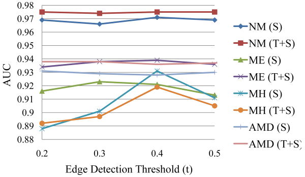
In the previous sections, we have established that $LB{P}_{8,1}^{\mathit{pca}}$ and MSSP are effective in encoding texture distribution in the retinal OCT images. We now evaluate the performance of different feature types–texture (T) alone, shape (S) alone, or in combination (TS). For shape features, we test the performance of several edge detection thresholds (t = 0.2, 0.3, …, 0.5). The AUC results under different edge detection thresholds t for S and TS are plotted in Fig. 9. The best AUC results achieved by each feature type are detailed in Table 8. For NM, ME, MH, and AMD, the best AUCs are 0.976, 0.939, 0.931, and 0.938, derived from the feature type setting: TS(t = 0.4), T, S(t = 0.4), and TS(t = 0.2), respectively.

Figure 9.

AUC results with respect to varied edge detection thresholds t when using S and TS features, respectively. MH is more sensitive to the settings of t than the other categories.

Table 8.

The AUC results of different feature types (T: texture, S: shape, TS: texture+shape) under the best edge detection threshold t, all with $LB{P}_{8,1}^{\mathit{pca}}$ (32) as the local descriptors. Significance test results are in the last column based on DeLong test at p = 0.05 level (>: left setting is better; ≈: comparable performance.)

AUC	T	S	TS	Sig. Test
NM	0.969 ±0.002	0.971 (t=0.4) ±0.002	0.976 (t=0.4) ±0.002	T ≈ S, TS > T, TS ≈ S
ME	0.939 ±0.004	0.923 (t=0.3) ±0.005	0.939 (t=0.4) ±0.004	T > S, TS ≈ T, TS > S
MH	0.846 ±0.011	0.931 (t=0.4) ±0.005	0.919 (t=0.4) ±0.005	S > T, TS > T, TS ≈ S
AMD	0.925 ±0.008	0.931 (t=0.2) ±0.005	0.938 (t=0.2) ±0.006	T ≈ S ≈ TS
Ave.	0.920	0.939	0.943

From Table 8, we find that for NM, TS significantly outperforms T though the absolute gain is small (0.7% in AUC); thus, including shape features can provide additional useful information. For ME, T and TS are significantly better than using S alone (1.6% AUC difference), but TS does not outperform T; this suggests that texture descriptors alone, which describe the distribution of intensity patterns, are discriminative enough for edema detection, e.g., detection of dark cystic areas embedded in lighter retinal layers. For MH, S is significantly better than using T or TS, with a large AUC difference (8.5%) between S and T. This reveals that using shape features alone is sufficient to capture the distinct contours of MH, while the details present in texture features might distract the classifier and harm the performance. For AMD, all three feature settings (T, S, TS) have no significant difference, but using combined features (TS) achieved the best performance, suggesting that both features types are beneficial.

Regarding the effects of edge detection thresholds t, in Fig. 9, we find that for NM, ME, and AMD, the AUC results under different t are all within 1% in AUC; but for MH, the performance is much more sensitive to the choice of t. In MH, we can see an apparent peak at t = 0.4, which retains relatively strong edges only, as shown in Table 1. When more weak edges are also included for MH (t < 0.4), the performance drops by a large margin (from 0.931 to 0.888 when t decreases from 0.4 to 0.2). This suggests that including weak edges is harmful for identifying the hole structures.

3.6. Discrimination of Sub-Categories within MH Category

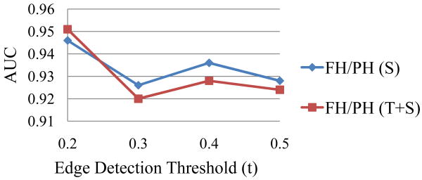
We evaluated the performance of our method in discriminating the subcategories, full-thickness holes (FH) and psedu-holes (PH), within MH category. The dataset statistics are listed in Table 9. The AUC results under varied edge detection thresholds t are plotted in Fig. 10. The best results for each feature type (T, S, TS) are detailed in Table 10.

Table 9.

The number of scans, eyes and subjects as defined by one expert ophthalmologist for full-thickness hole (FH) and pseudo-hole (PH) in MH category.

Statistics	FH	PH
Scan	39	35
Eye	17	15
Subject	17	18

Figure 10.

The AUC results with respect to varied edge detection thresholds (t) when using S and TS features for discriminating FH and PH.

Table 10.

The AUC results in discriminating FH and PH in MH category using different combination of feature types (T: texture, S: shape, TS: texture+shape) all with $LB{P}_{8,1}^{\mathit{pca}}$ (32) as the local descriptors. Significance test results are in the last column based on DeLong test at p = 0.05 level (>: left setting is better; ≈: comparable performance.)

AUC	T	S	TS	Sig. Test
FH vs. PH	0.871 ±0.015	0.946 (t=0.2) ±0.011	0.951 (t=0.2) ±0.011	S > T, TS > T, S ≈ TS

In Table 10, we find that S and TS perform significantly better than T (> 7% difference) while S and TS have no significant differences. Again, for distinguishing different hole structures, shape features are much more effective than textures, the same as in the parent category (MH). Regarding the edge detection thresholds t, in Fig. 10, we discover that there is a local peak at t = 0.4, the same as in MH category, but when t decreases to 0.2, the inclusion of weaker edges can provide a performance leap. This suggests that subtle shape structures captured by these weak edges are useful for sub-category discrimination. Overall, the high AUC results (0.951) demonstrate that the proposed feature representation is also effective at distinguishing similar-looking subtypes.

3.7. Visualization of Feature Weight Distribution of Linear SVMs

To gain insight into the characteristics of each pathology from the learning machine's perspective, we conduct a visualization experiment to show the spatial distribution of the most discriminative features of the learned SVMs.

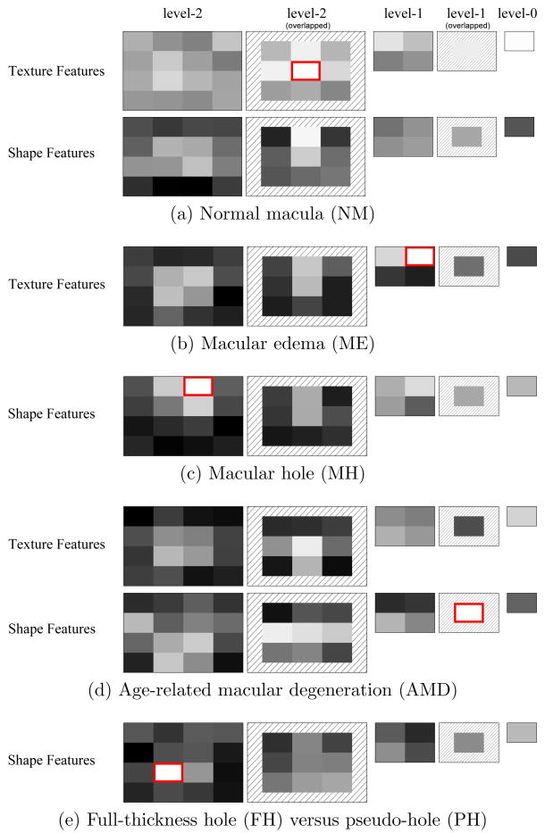
Our process and visualization scheme is as follows. For each pathology, we train a linear SVM using one fold of the training data and the best feature setting. After training, the weight value for each feature entry is derived. Then, for each spatial block, we compute the block's weight by summing up the absolute values of weights from features belonging to the block. For better visualization, we then map the highest block weight to 255, and lowest to 0. The brightest block, which is deemed the most discriminative, is enclosed by a red rectangle. The results are shown in Fig. 11.

Figure 11.

Visualization of feature weights of trained linear SVMs for each pathology. The block weights are rescaled to [0 255] for better visualization, with the brightest one enclosed by a red rectangle. (The feature setting is TS(t = 0.4) for NM, T for ME, S(t = 0.4) for MH, TS(t = 0.2) for AMD, and S(t = 0.2) for FH/PH).

From Fig. 11, we find that the most discriminative blocks are located at different pyramid levels for different pathologies. We also discover that for NM and ME, the brighter blocks are located around the central and top areas, which are the places for the normal, smooth depression or the hill shapes caused by the accumulated fluids. For MH, the top half areas, inhabited by the opening area of the holes, get higher weights. For AMD, the middle and bottom areas are brighter, corresponding to the normal or irregular bottom retinal layer (RPE layer). For FH/PH, the area around the central bottom retinal layer, which is the place revealing whether the hole touches the outermost layer, is heavily weighted.

The distribution of these feature weights is consistent with our intuition about the important areas for each pathology. This visualization experiment corroborates our initial hypothesis that SVM has the ability to discover the most discriminative features when given the full context, without the need for explicit feature selection beforehand.

4. Conclusion and Future Work

In this paper, we present an effective data-driven approach to identify normal macula and multiple macular pathologies, namely, ME, MH, and AMD, from the foveal slices in retinal OCT images. First, we align the slices to reduce their appearance variations. Then we construct a global image descriptor by using multi-scale spatial pyramid as the global representation, combined with dimension-reduced LBP histogram based on PCA as the local descriptor to encode both the retinal image and its edge map. This approach captures the geometry, texture, and shape of the retina in a principled way. A binary non-linear SVM classifier is then trained for each pathology to identify its presence. To further differentiate subtypes within the MH category, our method is also applied to distinguish full-thickness holes from pseudo-holes.

Our feature representation is novel for medical image analysis. Though LBP histogram has been applied in a variety of fields, to our knowledge, this is the first work using LBP^pca descriptor, as well as its use with the MSSP framework, in the medical domain. We have demonstrated that our feature representation outperforms other popular choices. In addition, our use of LBP^pca on the edge map for capturing the shape characteristics is first seen in the medical literature. This shape encoding has proven to be effective for MH identification.

We validate our approach by comparing its performance to that of using other common local descriptors and global representation. We then examine the effectiveness of using texture or shape features alone, or in combination, for identifying each pathology. We find that employing texture features alone is sufficient for ME while using shape features alone performs the best for identifying MH; for NM and AMD, utilizing both feature types achieves the best performance. To gain more insight from a learning machine's perspective, we visualize the learned feature weights to study the spatial distribution of the learned most discriminative features. The pattern of the weights is consistent with our intuition regarding the spatial location of specific pathologies. Our results demonstrate the feasibility of a global feature encoding approach which avoids the need to explicitly localize pathology-specific features within the OCT data.

Our method has several advantages. First, the histogram-based image features directly capture the statistical distribution of appearance characteristics, resulting in objective measurements and straightforward implementation. Second, the method is general, making it amenable to be extended to identify additional pathologies. Third, the same approach can be utilized to diagnose other cross sections besides the foveal slices, as long as the corresponding labeled slices from the desired anatomical locations are also gathered for training.

The limitation of the present work is that one foveal slice from a 3D SD-OCT scan, instead of the whole volume, was analyzed and that slice was manually selected (though in reality this slice is typically near the center in a macular scan.) Nevertheless, this study is designed as a foundation that can be easily applied to all other slices in the volume, with the fact that the foveal slice is the most informative one for identifying several common macular pathologies. Also, to our knowledge, our study is the first to automatically classify OCT images for various macular pathologies.

In future work, we plan to extend the method to analyze each slice in the entire macular cube. The most straightforward way is to train a set of y-indexed pathology classifiers, using labeled x-z slice sets from the same quantized y locations relative to the fovea. By using location-indexed classifiers, the normal and abnormal anatomical structures around similar y positions can be modeled more accurately, and each slice from the entire cube can be examined. Once the eye motion artifacts in the macular scans can be reliably corrected, we can further investigate the efficacy of volumetric features in pathology identification. We also plan to develop an automated method for fovea localization so that the entire process is fully-automatic.

In conclusion, an effective approach is proposed to computerize the diagnosis of multiple macular pathologies in retinal OCT images, which achieves AUC > 0.93 for all pathologies. Our method can be applied to diagnose every slice in the OCT volume. This may provide clinically-useful tools to support disease diagnosis, improving the efficiency of OCT-based ocular pathology identification.

• The first work in computer-aided diagnosis of macular pathologies in retinal OCT images

• The presence of normal macula and three pathologies (ME, MH, AMD) are identified

• A novel descriptor to encode geometry, texture, and shape of the retinal structures

• Extensive testing on large dataset of 326 scans with all AUC>0.93

• Machine learning based framework applicable to other pathologies

References

- Age-Related Eye Disease Study Research Group. A randomized, placebo-controlled, clinical trial of high-dose supplementation with vitamins C and E, beta carotene, and zinc for age-related macular degeneration and vision loss: AREDS report no. 8. Arch Ophthalmol. 2001;119:1417–36. doi: 10.1001/archopht.119.10.1417. [DOI] [PMC free article] [PubMed] [Google Scholar]
- Ahonen T, Hadid A, Pietikäinen M. Face description with local binary patterns: Application to face recognition. IEEE Trans on Pattern Analysis and Machine Intelligence. 2006;28:2037. doi: 10.1109/TPAMI.2006.244. [DOI] [PubMed] [Google Scholar]
- Barnum P, Chen M, Ishikawa H, Wollstein G, Schuman J. Local quality assessment for optical coherence tomography. IEEE Intl Symposium on Biomedical Imaging. 2008:392–395. [Google Scholar]
- Bosch A, Zisserman A, Munoz X. Representing shape with a spatial pyramid kernel. ACM Intl Conf on Image and Video Retrieval. 2007:401–408. [Google Scholar]
- Canny J. A computational approach to edge detection. IEEE Trans Pattern Analysis and Machine Intelligence. 1986;8:679–698. [PubMed] [Google Scholar]
- Chang CC, Lin CJ. LIBSVM: a library for support vector machines. 2001 Software available at http://www.csie.ntu.edu.tw/cjlin/libsvm.
- DeLong E, DeLong D, Clarke-Pearson D. Comparing the areas under two or more correlated receiver operating characteristic curves: a nonparametric approach. Biometrics. 1988;44:837–845. [PubMed] [Google Scholar]
- Freeman WT, Roth M. Orientation histogram for hand gesture recognition. Intl Workshop on Automatic Face and Gesture Recognition. 1994:296–301. [Google Scholar]
- Garvin MK, Abràmoff MD, Kardon R, Russell SR, Wu X, Sonka M. Intraretinal layer segmentation of macular optical coherence tomography images using optimal 3-D graph search. IEEE Trans on Medical Imaging. 2008;27:1495. doi: 10.1109/TMI.2008.923966. [DOI] [PMC free article] [PubMed] [Google Scholar]
- Ishikawa H, Kim JS, Friberg TR, Wollstein G, Kagemann L, Gabriele ML, Townsend KA, Sung KR, Duker JS, Fujimoto JG, Schuman JS. Three dimensional optical coherence tomography (3D-OCT) image enhancement with segmentation free contour modeling c-mode. Inves Ophthalmol Vis Sci. 2009;50:1344–9. doi: 10.1167/iovs.08-2703. [DOI] [PMC free article] [PubMed] [Google Scholar]
- Ishikawa H, Stein DM, Wollstein G, Beaton S, Fujimoto JG, Schuman JS. Macular segmentation with optical coherence tomography. Investigative Ophthalmology and Visual Science. 2005;46:2012–7. doi: 10.1167/iovs.04-0335. [DOI] [PMC free article] [PubMed] [Google Scholar]
- Lazebnik S, Schmid C, Ponce J. Beyond bags of features: Spatial pyramid matching for recognizing natural scene categories. IEEE Computer Vision and Pattern Recognition. 2006:2169–2178. [Google Scholar]
- Lee K, Niemeijer M, Garvin MK, Kwon YH, Sonka M, Abramoff MD. Segmentation of the optic disc in 3-D OCT scans of the optic nerve head. IEEE Trans Med Imaging. 2010;29:1321–1330. doi: 10.1109/TMI.2009.2031324. [DOI] [PMC free article] [PubMed] [Google Scholar]
- Liao S, Zhu X, Lei Z, Zhang L, Li SZ. Learning multi-scale block local binary patterns for face recognition. Intl Conf on Biometrics. 2007;4642:828–837. [Google Scholar]
- Liu YY, Chen M, Ishikawa H, Wollstein G, Schuman J, Rehg JM. Automated macular pathology diagnosis in retinal OCT images using multi-scale spatial pyramid with local binary patterns. Intl Conf on Medical Image Computing and Computer Assisted Intervention. 2010;6361:1–9. doi: 10.1007/978-3-642-15705-9_1. [DOI] [PMC free article] [PubMed] [Google Scholar]
- Luckie A, Heriot W. Macular holes. Pathogenesis, natural history, and surgical outcomes. Aust N Z J Ophthalmol. 1995;23:93–100. doi: 10.1111/j.1442-9071.1995.tb00136.x. [DOI] [PubMed] [Google Scholar]
- Ojala T, Pietikäinen M, Mäenpää T. Multiresolution gray-scale and rotation invariant texture classification with local binary patterns. IEEE Trans on Pattern Analysis and Machine Intelligence. 2002;24:971. [Google Scholar]
- Oliver A, Lladó X, Freixenet J, Martí J. False positive reduction in mammographic mass detection using local binary patterns. Intl Conf on Medical Image Computing and Computer Assisted Intervention. 2007;4791:286–293. doi: 10.1007/978-3-540-75757-3_35. [DOI] [PubMed] [Google Scholar]
- Quellec G, Lee L, Dolejsi M, Garbvin MK, Abramoff MD, Sonka M. Three-dimensional analysis of retinal layer texture: Identification of fluid-filled regions in SD-OCT of the macula. IEEE Trans Med Imaging. 2010;29:1321–1330. doi: 10.1109/TMI.2010.2047023. [DOI] [PMC free article] [PubMed] [Google Scholar]
- Ricco S, Chen M, Ishikawa H, Wollstein G, Schuman JS. Correcting motion artifacts in retinal spectral domain optical coherence tomography via image registration. Intl Conf on Medical Image Computing and Computer Assisted Intervention. 2009;5761:100–107. doi: 10.1007/978-3-642-04268-3_13. [DOI] [PMC free article] [PubMed] [Google Scholar]
- Schuman J, Pedut-Kloizman T, Hertzmark E. Reproducibility of nerve fiber layer thickness measurements using optical coherence tomography. Ophthalmology. 1996;103:1889–1898. doi: 10.1016/s0161-6420(96)30410-7. [DOI] [PMC free article] [PubMed] [Google Scholar]
- Schuman JS, Puliafito CA, Fujimoto JG. Optical Coherence Tomography of Ocular Diseases. Second 2004. [Google Scholar]
- Sørensen L, Shaker SB, Bruijne Md. Texture classification in lung CT using local binary patterns. Intl Conf on Medical Image Computing and Computer Assisted Intervention. 2008;5241:934–941. doi: 10.1007/978-3-540-85988-8_111. [DOI] [PubMed] [Google Scholar]
- The Eye Diseases Research Prevalence Research Group. The prevalence of diabetic retinopathy among adults in the United States. Arch Ophthalmol. 2004;122:552–63. doi: 10.1001/archopht.122.4.552. [DOI] [PubMed] [Google Scholar]
- Wu J, Rehg JM. Where am I: Place instance and category recognition using spatial PACT. IEEE Computer Vision and Pattern Recognition. 2008:1–8. [Google Scholar]
- Wu J, Rehg JM. CENTRIST: A visual descriptor for scene categorization. IEEE Trans on Pattern Analysis and Machine Intelligence. 2011 doi: 10.1109/TPAMI.2010.224. In Press. [DOI] [PubMed] [Google Scholar]
- Xu J, Ishikawa H, Wollstein G, Schuman JS. 3D OCT eye movement correction based on particle filtering. Intl Conf on IEEE Engineering in Medicine and Biology Society. 2010:53–56. doi: 10.1109/IEMBS.2010.5626302. [DOI] [PMC free article] [PubMed] [Google Scholar]