An Overview of Remote Sensing and Geodesy for Epidemiology and Public Health Application

Abstract

The techniques of remote sensing (RS) and geodesy have the potential to revolutionize the discipline of epidemiology and its application in human health. As a new departure from conventional epidemiological methods, these techniques require some detailed explanation. This review provides the theoretical background to RS including (i) its physical basis, (ii) an explanation of the orbital characteristics and specifications of common satellite sensor systems, (iii) details of image acquisition and procedures adopted to overcome inherent sources of data degradation, and (iv) a background to geophysical data preparation. This information allows RS applications in epidemiology to be readily interpreted. Some of the techniques used in geodesy, to locate features precisely on Earth so that they can be registered to satellite sensor-derived images, are also included. While the basic principles relevant to public health are presented here, inevitably many of the details must be left to specialist texts.

1. INTRODUCTION

1.1. Remote Sensing Definition

Remote sensing (RS) is the process of acquiring information about an object, area or phenomenon from a distance. This broad definition covers everything from the eyes reading this page to radio telescope installations that receive data that are processed to yield information from distant galaxies. The diversity of RS systems, however, can be usefully categorized as active or passive, differing simply in the source of the energy from which information is gathered. Active systems generate their own energy and passive systems rely on ambient energy from an external source which on Earth arises mainly from the Sun. In this chapter I shall consider both active (briefly) and passive (in depth) RS systems that measure the amount of radiant energy, i.e. the magnitude of electromagnetic radiation (EMR) reflected and radiated from the Earth’s surface and atmosphere, with a view to deriving information about surface conditions.

A recent review of the evolution of RS in the last two decades can be found in Cracknell (1999). There are numerous books devoted to RS and for general background to RS and its applications see, among others, Swain and Davis, 1978; Colwell, 1983; Curran, 1985; Asrar, 1989; Cracknell and Hayes, 1991; Cracknell, 1997a; Morain and Budge, 1997; Quattrochi and Goodchild. 1997; Sabins, 1997; Henderson and Lewis, 1998; Barrett and Curtis, 1999; Rencz, 1999; Richards and Jia, 1999; Gibson and Power, 2000a; Lillesand and Kiefer, 2000. Two useful books and tutorial CD-ROMs that provide image processing software, specimen data and examples of many of the procedures outlined in this chapter, can be found in Mather (1999) and Gibson and Power (2000b). The Idrisi32 geographic information system and image processing software also provides useful tutorials (Eastman, 1999a,b).

1.2. Electromagnetic Radiation

Electromagnetic radiation is emitted by all objects above absolute zero (0 K, −273°C) (see Plate 1a). The total amount of energy an object emits is expressed by the Stefan–Boltzman law which states that

$$M=\sigma T^4$$

where M is the total exitance (emitted radiant flux per unit area) from the surface of the material (W m⁻²), σ is the Stefan–Boltzman constant (5.6 × 10⁻⁸ W m⁻² K⁻⁴) and T is the absolute temperature of the emitting material (K). The total amount of energy emitted by an object therefore increases rapidly with temperature. This phenomenon is demonstrated by the larger area under the curve representing the electromagnetic spectrum (EMS) emitted by the Sun (at approximately 6000 K) than the corresponding area under the curve representing the EMS of the Earth (at approximately 300 K) (see Plate 1b). The figure also demonstrates the Wien’s displacement law, or the shift towards emission of shorter wavelengths by an object at higher temperature (Colwell et al., 1963; Monteith and Unsworth, 1990).

Plate 1.

(a) The electromagnetic spectrum (image courtesy of Dr R. Douglas Ramsey, Utah State University), (b) The spectral characteristics of Sun and Earth electromagnetic radiation sources (bottom graph) and atmospheric sinks (top graph). Note that the wavelength scale is logarithmic. IR, infrared; UV, ultraviolet. See Hay (this volume).

1.3. Atmospheric Transmittance, Spectral Response and Radiometer Design

Satellite-borne radiometers (or sensors) are instruments for measuring the intensity of EMR within a narrow range of wavelengths (or waveband), the resulting electronic signal from which, when processed, is often referred to as a channel. The measured EMR must travel through the atmosphere, which both scatters and absorbs EMR. These interactions are most significant close to the Earth’s surface (~1–5 km) in the atmospheric boundary layer (ABL). Due to such interactions, atmospheric transmission of EMR is wavelength-dependent (see Plate 1b, top graph). Consequently, radiometers are often designed to maximize the information content of the signal received by operating in ‘atmospheric windows’ of maximal EMR transmission, thus reducing the effect of atmospheric attenuation.

The interaction of the EMR with the Earth surface (reflected, absorbed or transmitted), and what we can infer about surface properties from this interaction, is the essence of remote sensing. The reflected portion varies with both the material observed and the wavelength of EMR with which the measurement is taken. The composite nature of the reflected components is often referred to as a spectral response pattern (or signature). For example, the spectral response pattern of the ink on this book is designed to absorb EMR across a range of wavelengths and the page itself to reflect so that our eyes perceive a large contrast between black and white respectively, which makes for easy reading. The ideal, that each material on Earth be characterized by a unique spectral signature, is rarely achieved. Multi-temporal information and further processing of data into geophysical information can often assist in this discrimination and is discussed further (see also Curran et al., this volume; Rogers, this volume; Goetz et al., this volume).

2. ACTIVE REMOTE SENSING

Radar (radio detection and ranging) RS is the sub-set of active RS that is potentially useful in public health. Radar RS operates in the microwave proportion of the electromagnetic spectrum, generally considered to be at wavelengths of 1 mm to 1 m. Most modern radar sensors incorporate software routines on the sensor to improve spatial resolution mathematically and to cope with multiple pictures of the same object, and are hence referred to as Synthetic Aperture Radars (SARs) (Brown and Porcello, 1969; Sarder, 1997). SAR sensors are unique in that they can determine the polarization (horizontal or vertical) of electromagnetic energy they emit and receive, allowing increased information on retrieval surface properties. The atmosphere has almost complete transmittance at microwave wavelengths (see Plate 1b, top graph), and radar wavelengths are so resistant to atmospheric attenuation that images can be generated even through cloud. Furthermore, radars generate their own energy so they can operate day and night independent of solar insolation. These characteristics would seem to provide ideal data for a range of RS applications, but several factors have contributed to SAR image interpretation remaining a specialist discipline (Waring et al., 1995; Kasischke et al., 1997). These are (i) the difficulty of interpreting the information content of SAR imagery (see, for example, Oliver, 1991), (ii) historically the relative lack of calibrated SAR data over areas of interest, (iii) the lack of software to automate handling of the data generated, and (iv) the unique problems involving topography and image speckle. The specific capabilities of various sensors and polarizations have been considered by Schmullius and Evans (1997) and those of interest to public health include accurate classification and detection of change in land-cover, excellent discrimination of flooding extent and water bodies, and also soil moisture status (Waring et al., 1995; Kasischke et al., 1997). The routine use of SAR data in public health is not imminent and hence not evaluated in detail, but for the adventurous a daunting yet comprehensive starting point is Henderson and Lewis (1998).

3. PASSIVE REMOTE SENSING

3.1. Airborne Sensor Systems

The principals of RS from airborne and satellite platforms are very similar. To avoid duplication within this review I shall focus specifically on satellite sensor systems. Moreover, some aspects of airborne RS are detailed more fully by Curran et al. (this volume).

3.2. Satellite Sensor Systems

Radiometers can be carried on two broad categories of satellite, geostationary and polar-orbiting. Geostationary satellites are put into a high altitude orbit (~23 000–40 000 km) at the equator, with a speed equal to that of the Earth’s rotation, so that they remain fixed above a particular point on Earth. Polar-orbiting satellites circle the globe repeatedly at much lower altitude orbits (~600–900 km) roughly perpendicular to the equator. Successive orbits therefore pass over a different section of the Earth as it rotates (Cracknell and Hayes, 1991).

Sensors receive EMR from the cone within which energy is focused on the detector (Figure 1). The relationship between the angle of this cone at the sensor (in radians), also called the instantaneous field of view (IFOV), β, the height of the sensor above the Earth, H, and the resulting diameter of the viewing area, D, often referred to as the spatial resolution, is given by:

$$D=H\beta$$

For example, the spatial resolution of the National Oceanic and Atmospheric Administration—Advanced Very High Resolution Radiometer (NOAA-AVHRR) with an average IFOV of 1.4 milliradians and an orbiting altitude of approximately 833 km can be found from the above equation as D = 833 000 × (1.4 × 10⁻³) = 1166 m; close to the 1.1 km often quoted (Kidwell, 1998).

Figure 1.

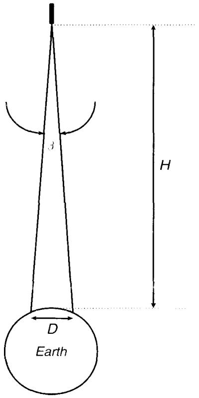
A schematic diagram of the factors affecting the spatial resolution of a radiometer. The instantaneous field of view (IFOV), β, is measured in radians; the height of the sensor above the Earth, H, and the resulting diameter of the viewing of the Earth, D, are measured in metres.

The data from satellite sensors are stored and transmitted as digital numbers, with each value referring to the smallest area for which the satellite sensor can record data. When viewed on a computer monitor these areas are called picture elements or ‘pixels’. The assumption that for each pixel the digital number represents the mean spectral signal from all objects within the IFOV is generally correct for those sensors that try and match the pixel to the IFOV (Price, 1982) but this is a more complicated issue than it might first appear (Cracknell, 1998).

In polar-orbiting satellites the sensor scans across the track of the satellite as the orbit progresses to generate a series of contiguous scan lines which, when combined, form a two dimensional image (or scene). In geostationary satellites the radiometer itself must move perpendicularly to the plane of the scan line at regular intervals to generate the image. The swath width (breadth of the area over which data are recorded by a sensor) is determined by both the satellite altitude and sensor characteristics. For example the NOAA-AVHRR scans to ±55.4° from the point of Earth directly under the satellite (its nadir) which, at an altitude of approximately 833 km, results in a swath width of approximately 2700 km. Due to the curvature of the Earth, the effective distance between the Earth and the sensor increases with the scan angle so that the spatial resolution decreases to approximately 4 × 4 km toward the edge of the swath.

The repeat time, or the time taken between viewing the same part of the Earth’s surface, varies between satellite systems and is determined by a combination of the swath width and orbital characteristics. Furthermore, data volume of satellite sensors is constrained by on-board storage media (especially in older satellites) and the limited opportunity for telemetry (transmission of data between satellite and receiving station) during the satellite overpass, so that RS images tend to have either a high-temporal resolution or a high-spatial resolution, but not both. Satellite sensor data therefore are limited in their spectral, spatial and temporal resolution by a variety of factors which reflect the compromise between the constraints of atmospheric effects, engineering limitations and the desired application. The compromises reached between the spectral, spatial and temporal resolutions by some of the satellite sensor systems currently used in public health applications are detailed in Tables 1 and 2, although advances in satellite sensor technology are constantly improving specifications and increasing the amount of data that can be generated, stored and transmitted.

Table 1.

The spectral, spatial and temporal resolution of high spatial resolution satellite sensors systems. See Morain and Budge (1997) for a more comprehensive list.

Satellite sensor system	Resolution
	Spectrala (μm)	Spatialb (m)	Temporal (days)
Landsat-1, -2,-3 Return Beam Vidicon (RBV) camera	Ch 1–3 (0.475–0.830)c	79	18
Landsat-1, -2, -3, -4,-5 Multispectral Scanner (MSS)	Ch 4–7 (0.5–1.1),d	79/82e	16/18
Landsat-4, -5 Thematic Mapper (TM)	Ch 1–5 and 7 (0.45–2.35)	30	16
	Ch 6 (10.40–12.50)	120
Landsat-6f, -7 Enhanced Thematic Mapper+ (ETM+)	Ch 1–5 and 7 (0.45–2.35)	30	16
	Ch 6 (10.40–12.50)	60
	Ch P (0.50–0.90)	15
Satellite pour l’Observation de la Terre-1, -2, -3 (SPOT) High Resolution Visible (HRV) Panchromatic Mode (HRV-PAN) Multispectral Mode (HRV-XS)	Ch I (0.51–0.73)	10	26g
	Ch 2–4 (0.50–0.89)	20
SPOT-4 High Resolution Visible and Infrared (HRVIR)	Ch 1 (0.61–0.68)	10	26g
	Ch 2–5 (0.50–1.75)	20
Terra Moderate Resolution Imaging Spectroradiometer (MODIS)	Ch 1–2 (0.620–0.876 )	250	1–2
	Ch 3–7 (0.459–2.115)	500
	Ch 8–36 (0.405–14.385)	1000

^aThe spectral resolutions are the electromagnetic wavelength range in μm where 0.3 is at the visible and 14 at the thermal infrared end of the spectrum (Plate 1a).

^bThe spatial resolution is given as the diameter of the viewing area of the sensor, D, at nadir.

^cLandsat-3 had a fourth panchromatic RBV channel (0.505–0.750) at a 40 m spatial resolution.

^dLandsat-3 had an eighth MSS thermal channel (10.4–12.6) at 237 m spatial resolution.

^eThe spatial resolution is 79 m for Landsat-1 to -3 and 82 m for Landsat-4 and -5 since the satellite altitude changed from 920 km to 705 km. The temporal resolution also changed accordingly.

^fLandsat-6 never achieved orbit and Landsat-7 is currently in operation.

^gA pointing facility can increase the frequency of coverage.

Table 2.

The spectral, spatial and temporal resolution of low spatial resolution satellite sensors systems. See Morain and Budge (1997) for a more comprehensive list.

Satellite sensor system	Resolution
	Spectrala (μm)	Spatialb(km)	Temporal (h)
National Oceanic and Atmospheric Administration (NOAA)
Advanced Very High Resolution Radiometer (AVHRR)	Ch 1–5 (0.58–11.50)	1.1	12
Meteosat-4, -5, -6
High Resolution Radiometer (HRR)	Ch 1 (0.40–1.10) Ch 2–3 (5.70–12.50)	2.5 5	0.5
Meteosat Second Generation-1 (MSG)c
Spinning Enhanced Visible and Infrared Imager (SEVRI)	Ch 1 (0.6–0.9) Ch 2–12 (0.56–14.4)	1 3	0.25

^aThe spectral resolutions are the electromagnetic wavelength range in μm where 0.3 is at the visible and 14 at the thermal infrared end of the spectrum (Plate 1a).

^bThe spatial resolution is given as the diameter of the viewing area of the sensor, D, at nadir.

^cDue to he launched at the end of 2000.

3.2.1. High Spatial Resolution Sensors

In this review and throughout subsequent chapters, the ability to resolve areas smaller than 1 × 1 km is used as an arbitrary criterion for defining high spatial resolution sensors. The lower frequency of image capture for any point on the Earth for high spatial resolution satellite sensors means that such satellites sensors give few cloud-free images of the Earth’s surface per year, especially over tropical regions. This, together with the cost of such imagery, has generally limited application of high-spatial resolution imagery to the production of habitat maps for relatively small areas and for a particular season of the year. The following examples do not form a comprehensive survey, particularly for very recent sensors which have not yet been adopted in public health application. Those sensors from which data are very difficult to obtain are also excluded. A more complete list of high spatial resolution satellite sensors is available (Morain and Budge, 1997).

(a) The Landsat Series

The launch of Landsat-1 in 1972 heralded a new era of high resolution RS, and changed the perception by experts and lay people alike of the possible ways in which to view the Earth (Lauer et al., 1997; Lowman, 1999). The Landsat programme has generated a continuous supply of high resolution imagery, for the entire globe, from the first Multispectral Scanner (MSS) aboard Landsat-1 to the latest Enhanced Thematic Mapper (ETM +) on board Landsat-7 (Mika, 1997) (Table 1). In so doing, it has offered unique insights into global terrestrial phenomena (Goward and Williams, 1997). During this time there has been a substantial evolution in the quality of the radiometers (Mika, 1997), their calibration (Thome et al., 1997) and the development of multispectral data analysis techniques developed to process captured data (Landgrebe, 1997), all of which will continue (Ungar, 1997). Moreover, the novelty and conspicuous success of the Landsat programme forced issues regarding data distribution and cost (Draeger et al., 1997) and the feasibility of commercial RS (Williamson, 1997) to be considered seriously for the first time. Many countries have understandably emulated and extended features of the Landsat programme, and other high resolution RS data sources are now increasingly available (Morain and Budge, 1997).

(b) The SPOT Series

The French Satellite pour l’Observation de la Terre (SPOT) programme began in 1986 with the launch of SPOT-1 with the High Resolution Visible (HRV) sensor payload (Table 1). Data have been collected continuously since this time with SPOT-4, carrying the High Resolution Visible and Infrared (HRVIR) sensor that is now in operation. There are many similarities between these data and Landsat-TM imagery, but SPOT-HRV achieves a slightly higher spatial resolution with fewer spectral channels. Data accessibility, the degree of cloud contamination on scenes of interest, and cost, all help determine a researcher’s choice between the different sorts of high resolution imagery available.

3.2.2. Low Spatial Resolution Sensors

In contrast to the sensors on board Landsat and SPOT, the sensors on board the NOAA series of polar-orbiting meteorological satellites and the Meteosat series of geostationary satellites have relatively high-temporal and low-spatial resolutions. The advantages of these features are detailed extensively in the following chapters and have led to these systems being very widely utilized by the RS community (Cracknell, 1999). Furthermore, these data are available free in the public domain to research institutes and will soon have increased spectral, temporal and spatial coverage (Hay et al., 1996) (see Section 3.3).

(a) The NOAA Satellite Series

The NOAA series of polar-orbiting Television Infrared Observation Satellites (TIROSs) has been operational since 1978 (Hastings and Emery, 1992; Cracknell, 1997g). TIROS-N (later renamed NOAA-6) was the first satellite to carry the AVHRR and has been followed by seven satellites each achieving an operational lifetime of between 2 and 4 years. The ‘very high resolution’ refers to the 10 bit radiometric resolution of the sensor, which therefore has the ability to store data in the zero to 1023 range. The definitive description of the NOAA polar-orbiting satellites, their radiometer payloads and the data they generate is given in Kidwell (1998).

The NOAA satellites complete 14.1 near-polar, Sun-synchronous orbits per day at an altitude of 833–870 km. Since the number of orbits is not an integer, the orbital track over the Earth does not repeat on a daily basis. The even-numbered satellites have an ascending node with a north-bound equatorial crossing during the evening (19:30 Local Solar Time (LST)) and a descending node with a south-bound equatorial crossing in the morning (07:30 LST), whereas the odd-numbered satellites have an ascending node in the afternoon (14:30 LST) and a descending node at night (02:30 LST). At present the exception is the latest NOAA-14 satellite, launched in December 1994, which replaces NOAA-13 in functionality and thus has a daytime ascending node (Cracknell, 1997g).

As we have discussed, the NOAA-AVHRR can view a 2400 km swath of the Earth and, at this orbital frequency, daily data are recorded for the entire Earth surface. Radiation is measured in five distinct wavebands of the EMS so that five separate waveband images are recorded for each orbit (Table 2). The visible channel 1 and near infrared (NIR) channel 2 measure reflected solar radiation whereas the thermal channels 4 and 5 measure emitted thermal infrared (TIR). Channel 3, in the mid infrared (MIR), is a hybrid and sensitive to a combination of both reflected and emitted radiances.

The spatial resolution of the AVHRR is approximately 1.1 km beneath the track of the orbiting satellite (see Section 3.2). These nominal 1.1 km AVHRR data are continuously transmitted and may be received by stations along or near to the satellite’s path, where they are referred to as high resolution picture transmission (HRPT) data (Cracknell, 1997d). On request to NOAA these data may also be recorded on an on-board tape storage system and later transmitted to Earth as the satellites pass over a network of receiving stations. The data are then referred to as Local Area Coverage (LAC) data. These 1.1 km data have found application in a very wide range of disciplines and are reviewed by Ehrlich et al. (1994) and Cracknell (1997b).

Two processing steps further reduce the spatial resolution of most of the AVHRR data available to the user community. The on-board tape system is incapable of holding global coverage data at 1.1 × 1.1 km spatial resolution. Instead, the information from each area of five (across-track) by three (along-track) pixels is stored as a single value, the average of the first four pixels only of the first row of the 5 by 3 block. The resulting imagery is referred to as Global Area Coverage or GAC data. GAC data, with a stated nominal spatial resolution of 4 × 4 km, are obviously far from ideal representations of the raw data (Justice et al., 1989) and their method of sub-sampling has consequences for environmental modelling (Belward and Lambin, 1990; Belward, 1992). Nevertheless, GAC data are the form in which most of the AVHRR archive was collected and reasonable quality global data sets are available at a variety of spatial resolutions (4 × 4 km or coarser) from the early 1980s to date (Townshend and Tucker, 1984).

(b) The Meteosat Satellite Series

The European Organization for the Exploitation of Meteorological Satellites (EUMETSAT) geostationary Meteosat satellite series began with the launch of Meteosat-1 in 1977 (Morain and Budge, 1997). Experimental satellites were used until the launch of the first operational satellite, Meteosat-4, in June 1989. The spin-stabilized satellites are put into orbit at an altitude of 35 800 km over the Gulf of Guinea, at the crossing of the Equator and the Greenwich meridian (0°N, 0°E). In this position, images are captured for the full Earth’s disc including Africa, Europe and the Middle East. A reserve satellite operates nearby in a standby condition (Anonymous, 1971).

The principal payload of the satellite is a High Resolution Radiometer (HRR). The radiometer operates in a broad visible waveband (channel 1), a thermal infrared waveband (channel 2) and a water vapour absorption infrared waveband (channel 3) (Table 2). The Meteosat satellites were designed for meteorological applications, so channel 3 is located in the thermal infrared area of maximal water vapour absorption and hence is ideal for monitoring clouds. At nadir the spatial resolution is 2.5 × 2.5 km for the visible images and 5 × 5 km for the thermal infrared and water vapour images. Further from the equator, the spatial resolution decreases so that over northern Europe it is 4 × 4 km in the visible wavebands and 8 × 8 km in the thermal infrared and water vapour wavebands. Each image is transmitted to the Earth in real time as each scan line is completed and new images are generated at 30-minute intervals (WMO, 1994).

3.3. Future Satellite Sensors

There are many planned enhancements to the satellite sensor systems described above (Beck et al., 2000; Wood et al., this volume). These improvements tend to be frequently modified and are therefore best reviewed at the relevant internet addresses for each satellite sensor series (Table 3). Of particular interest to those interested in RS applications in African public health will be the EUMETSAT Meteosat Second Generation (MSG) satellites that will carry the Spinning Enhanced Visible and Infrared Imager (SEVRI) (Battrick, 1999). Located in the same geostationary orbit as the existing Meteosat satellites, the MSG-SEVRI will provide 1 × 1 to 3 × 3 km spatial resolution images at 15 minute intervals in 12 spectral wavebands, ranging from 0.56 μm in the visible to 14.4 μm in the infrared domain. This increases significantly the capabilities of this satellite sensor series, the main advantage being the frequency of data collection allowing less attenuated images to be rapidly composited on a daily or weekly basis (see Section 4.2).

Table 3.

Useful universal resource locators (URLs) for common satellite sensor systems, image processing software and GPS manufacturers. The table is not comprehensive and does not endorse any specific company or product.

Remote sensing satellite systems
Landsat	http://landsat.gsfe.nasa.gov
SPOT	http://www.spotimage.fr
Terra	http://terra.nasa.gov
NOAA-AVHRR	http://daac.gsfc.nasa.gov/CAMPAIGN DOCS/LAND_BIO/GLBDST_main.html
Meteosat / MSG	http://www.esa.int/satellites
Image processing software
EASI/PACE	http://www.peigeomatics.com
ENVI	http://www.envi-sw.com
ERDAS	http://www.erdas.com
ER Mapper	http://www.ermapper.com
TNTmips	http://www.microimages.com
WinDisp	http://www.fao.org/giews/english/windisp/windisp.htm
Hand-held GPS manufacturers
Garmin	http://www.garmin.com
Magellan	http://www.magellangps.com
Trimble	http://www.trimble.com

In addition to improvements of existing satellite sensor series, new systems are also being continually developed. An example that will be widely adopted in public health is NASA’s Terra, which will generate imagery with a range of on-board sensors, most noticeably the Moderate Resolution Imaging Spectroradiometer (MODIS) (Table 1). Benefits to RS applications will be threefold. First the range of data available will increase substantially with 36 spectral channels from which more accurate meteorological and other ecological variables may be derived. Moreover, the channels have been designed with smaller waveband ranges to exploit ‘spectral windows’ where atmospheric signal attenuation is minimal and will therefore have significantly improved signal-to-noise ratios. Secondly, MODIS will have a high temporal resolution (two-day repeat time) at significantly higher spatial resolution (250 × 250 to 1000 × 1000 m depending on the channel) than existing sensors, in effect resulting in hybrid data with characteristics of both the NOAA-AVHRR and Landsat-TM. Thirdly, the stated aim is to ingest, process and disseminate data within three days of acquisition, including many potentially useful products, such as improved spectral vegetation indices, land surface temperature and evapotranspiration estimates. This means that much of the routine data processing will be performed at source giving unparalleled, rapid access to contemporary data on large-area ecosystem processes.

This section is not intended to be comprehensive, as future advances in remote sensing pertinent to epidemiology are dealt with in more detail by Goetz et al. (this volume) and Myers et al. (this volume).

4. TURNING SATELLITE SENSOR DATA INTO GEOPHYSICAL DATA

This section details some of the fundamental problems experienced by an orbiting satellite sensor in the measurement of reflected and radiated EMR from a curved surface, through an atmosphere of spatially heterogeneous composition. It then deals with how such data are converted into calibrated geophysical variables at known geographical locations. At this stage we introduce the caveat that the information presented in Sections 4 and 5 is orientated toward the NOAA-AVHRR sensor. This is because the author’s experience of remote sensing stems primarily from using such data and many of the future applications of RS in public health will utilize these and related satellite data. Thus, in many cases, while the exact details may not be accurate for a different satellite sensor system, the process of obtaining useful information from satellite-sensor-derived digital data will be informative. It is acknowledged that many applications in public health have been concerned with the classification of land cover and its extent, using single scenes. These aspects of remote sensing are considered in more depth by Curran et al. (this volume).

4.1. Image Registration

Raw digital data derived from satellite sensors need to be pre-processed geometrically to rectify (or register) them, usually to a base map at a particular scale and in a particular map projection (Snyder, 1987), or to other images in a series for monitoring change (also sec Section 6). Registration is generally an automated process that uses an ephemeris model of the orbital parameters of the satellite and a time signal sent down with the satellite sensor imagery to predict the satellite’s position relative to the Earth at the time of image capture (Brush, 1988; Emery et al., 1989; Baldwin and Emery, 1995). Algorithms for positional calculations originally assumed that the satellites were in their correct attitude and were following precisely their intended orbits. Unfortunately, this is not the case, since satellites vary considerably in both their orbit and attitude (McGregor and Gorman, 1994). An extreme example is that the equator crossing time for NOAA-11, which was 14:20 LST when the satellite was launched in February 1985, had drifted to 16:07 LST by November 1988 (Kidwell, 1998). These deviations from design values, and variations in these deviations, mean that some of the resulting imagery is not accurately registered to the appropriate base maps.

Satellite sensor images also suffer from geometric distortions due to other factors which include: panoramic distortion, Earth curvature, atmospheric refraction, relief displacement and non-linearities in the sensor’s field of view (Lillesand and Kiefer, 1994). These errors may be systematic or random. Geometric correction of systematic errors is usually done by modelling the sources of errors mathematically and applying the resulting corrective formulae (Wu and Liu, 1997).

Random distortions are overcome by measuring the shift of ground control points (GCP), distinctive geographical features of known location on the image, and resampling or reforming the original image to a new one accordingly. The functional relationship (f) between the X and Y file co-ordinates of the original satellite sensor image and the known latitude (x) and longitude (y) are determined by a least squares regression to determine the coefficients for two co-ordinate transform equations:

$$\begin{array}{cc}\hfill & X=f_1(X,Y)\hfill \\ \hfill & Y=f_2(X,Y)\hfill \end{array}$$

After a geometrically correct geographical grid is defined in terms of the longitude and latitude, each cell in this grid is given values of x and y according to the co-ordinate transform equations above. The computer then maps the digital number from the pixel closest to this address in the raw image to the geometrically correct geographical grid. This last step can be done in a simple way, such as to the nearest neighbouring pixel, or by using more sophisticated and computer intensive methods, such as bilinear and cubic spline interpolations (Khan et al., 1992, 1995). These spatial interpolation processes, however, may substantially alter the radiometric fidelity of the data so must be considered carefully (Goward et al., 1991). The most recent systems developed for NOAA-AVHRR image navigation use an ephemeris model and GCP-based rectification simultaneously (Marçal, 1999).

The on-board sensors of geostationary satellites view the Earth as a disc, so that apart from spherical distortion there are few, if any, problems of geo-registering such images. The raw data from polar-orbiting satellite sensors, however, are a scries of strips that must be co-registered and geometrically corrected before successive images can be joined together.

Image registration to a map can involve a loss of spatial resolution, the extent of which is usually increased to allow for the coarsest spatial resolution of the data rather than over sampling at the nadir pixel size. Final registration to a base map frequently has to be performed by visual inspection of the image with a map overlay (Krasnopolsky, 1994). The effects of these various stages of image resampling on NOAA-AVHRR data are considered in Khan et al. (1995) and reviewed in detail in Cracknell (1997f).

4.2. Reducing Cloud Contamination

Each of the high-temporal resolution images from the NOAA (and Meteosat) satellite sensors is as affected by cloud contamination as any single Landsat or SPOT sensor image, but their much higher frequency means that data quality can be improved by combining images over a relatively short period of time by compositing. The aim of compositing is to choose the most cloud free and/or least atmospherically contaminated radiance value within the compositing period.

Most compositing algorithms rely on the fact that one common image product from the NOAA-AVHRR, the Normalized Difference Vegetation Index (NDVI), produced from channels 1 and 2 (see Section 5.1 for details), has values that are generally reduced by cloud and other atmospheric contamination (Holben, 1986; Kaufman and Tanré, 1992). The highest NDVI values recorded during any relatively short time period are therefore thought to occur when cloud cover is least, and such values are taken to represent the least attenuated pixel value for the period. This method of image production is called maximum value compositing (MVC), and is usually carried out over a ten-day (decadal) compositing period. It has the important consequence that maximum image values for adjacent pixels in a single image may have been collected on different days during the compositing period. MVC methods tend to degrade still further the spatial resolution of the final image product, primarily for geo-referencing reasons (Meyer, 1996; Robinson, 1996) so that the recorded value for any nominal 8 × 8 km pixel may in fact have been drawn from an area as large as 20 × 20 km. Further problems associated with MVC and alternatives are outlined in Stoms et al. (1997), but have not been widely acknowledged.

Selection of the least cloud-contaminated images in the other AVHRR channels usually depends upon the selection of the NDVI date chosen by MVC. The same image that is used to generate the NDVI for any pixel is also taken as the source of information for the other AVHRR channels for that pixel and period. Increasingly in land applications over the tropics, however, AVHRR channels 4 and 5 are composited separately, i.e. without reference to the NDVI, since the overlying clouds are generally colder than the land so that the highest thermal value in the series will probably be the least cloud contaminated (Lambin and Ehrlich, 1995, 1996).

4.3. Reducing Other Atmospheric Effects

During image registration to a base map, other corrections for atmospheric effects such as Rayleigh scattering caused by aerosols and absorption by water vapour, carbon dioxide and ozone, may also be applied, using ancillary information in the data stream from the satellite sensor (Vermote et al., 1990; Tanré et al., 1992). This is very important because atmospheric aerosols, which are highly spatially and temporally variable in the atmosphere (Holben et al., 1991), scatter light particularly at short visible wavelengths (i.e. NOAA-AVHRR channel 1), whilst atmospheric water vapour absorbs particularly in the near infrared (i.e. NOAA-AVHRR channel 2) (Kaufman and Tanré, 1992). If corrections for atmospheric effects are not made at the time of image registration they generally cannot be made as accurately at a later stage. Instead, corrections are based on average values for a ‘standard’ atmosphere within a region (Hanan et al., 1993; Goetz et al. 1995). Despite attempts to remove the effects of clouds and other contaminants by MVC of AVHRR imagery, continuous total or sub-pixel cloud cover and haze may still affect MVC images.

4.4. Satellite Sensor Drift

During their operational lifetime the AVHRR sensor characteristics change with use and as their components age (Gorman and McGregor, 1994) so that external or ‘vicarious’ calibration is required. The TIR channels are continuously calibrated against the 4 K space background temperature, measured by a thermistor on the baseplate of the satellite. Channels 1 and 2 are calibrated by making simultaneous measurements with aircraft under-flights (Smith et al., 1988), or by examining the change in signal from relatively invariant reflectors such as deserts and high clouds, or from invariant reflective phenomena such as the molecular scattering of the visible signal over oceans and areas of sun glint (Che and Price, 1992; Kaufman and Holben, 1993). Correction factors can also be added to spectral vegetation indices (SVIs) without recourse to the visible channel data by assuming a linear degradation in sensor response, examples of which are given by Los (1993) for the NDVI. It should suffice to note that calibration is currently a contested term in RS and for those interested in the debate, guidelines can be found at http://www.tandf.co.uk/journals.

4.5. Satellite Orbit Drift

Even when corrections for atmospheric effects and instrumental drift have been made, the resulting imagery may still show periodic changes in the signal due to a precession of the satellite’s orbit known as phasing. This results in cyclical variation of over-pass times, which, in the case of NOAA-AVHRR imagery, have a 17-day cycle (McGregor and Gorman, 1994). Signal variation can therefore be due to the changing angles between the Sun, the Earth and satellite sensors. Moreover, afternoon equitorial overpass times become progressively later after launch, causing artefactual ‘cooling’ trends in the brightness temperature time series (Price, 1991) because measurements occur later in the afternoon. Recent work has suggested elegant solutions to these problems for long-term archived RS data sets (Gutman, 1999a,b; Gleason et al. 2000).

5. TURNING GEOPHYSICAL DATA INTO INFORMATION FOR PUBLIC HEALTH

The previous section highlighted the problems of obtaining geographically registered satellite sensor data and the sources of error involved in the processes. This section describes how such information can be converted to vegetation, land surface temperature, atmospheric moisture and rainfall indices. The accuracy with which meteorological variables can be described is also discussed. The most recent advances and a more in-depth consideration of some of these issues are provided by Goetz et al. (this volume).

5.1. Spectral Vegetation Indices

Most SVIs (reviewed by Huh, 1991; Myneni et al., 1995b; Cracknell, 1997h; Lyon et al., 1998) exploit the fact that chlorophyll and carotenoid pigments in plant tissues absorb light in the visible red wavelengths (which corresponds to AVHRR channel 1), whereas mesophyll tissue reflects light in the near infrared wavelengths (which corresponds to AVHRR channel 2) (Sellers, 1985; Tucker and Sellers, 1986). A healthy and actively photosynthesizing plant will therefore look darker in the visible, and brighter in the near-infrared region, than an unhealthy or scncscing plant. Furthermore, as vegetation coverage increases, there is more absorption of red radiation due to the increasing amount of pigmentation and more reflectance of near-infrared radiation due to increases in internal leaf scattering of mesophyll (Curran and Williamson, 1986). The reflectance from dry soil is less complex than that of vegetation, showing a general increase in reflectance with wavelength which is dependant on soil texture, structure, and water, organic carbon and iron oxide content (Huete and Escadafal, 1991). Since soils and vegetation exhibit very different spectral properties these features are used to differentiate between the two types of surfaces. SVIs are simply designed to maximize the contrast in reflectance and thereby identify the presence of vegetation in RS images.

The most simple SVI is the ratio of AVHRR channel 2 (Ch₂) over channci 1 (Ch₁) reflectances, called the ratio vegetation index (RVI) or simple ratio index (SRI). Other SVIs attempted to overcome the problem of reflectance from the (usually dark or reddish) soil backgrounds by dividing the difference between these two channels by their sum, to give the NDVI (Tucker, 1979), defined as follows:

$$\mathrm{NDVI}=\frac{({\mathit{Ch}}_2-{\mathit{Ch}}_1)}{({\mathit{Ch}}_2+{\mathit{Ch}}_1)}$$

The values of the NDVI can theoretically range from −1 to +1, but in practicc usually fall within 0.0–0.8 limits (Colwell, 1974; Tucker, 1979; Tucker et al., 1991). The NDVI, in common with all red/near-infrared indices, is a specific measure of chlorophyll abundance and light absorption (Myneni et al., 1995a), but its use has been extended to quantify herbaceous vegetation biomass (Tucker et al., 1983, 1985b), vegetation primary productivity (Prince and Goward, 1995; Goetz et al., 1999), vegetation coverage (Tucker et al., 1985a; Goetz, 1997) and phenology (Justice et al., 1985) in a range of ecosystems. NDVI measurements are particularly useful in areas of sparse vegetation coverage, where they have a larger dynamic range than the simpler SVIs such as RVI. The NDVI does, however, saturate in areas of full coverage such as forests (Huh, 1991). It is also less than ideal because of continuing problems with background soils (which are, for example, darkened by rainfall (Huete et al., 1985)) and differential atmospheric effects on channel 1 and 2 radiances.

Alternative indices have been suggested to overcome some of these problems (Jackson and Huete, 1991; Leprieur et al., 1996) such as the soil adjusted vegetation index (SAVI) (Huete, 1988) and the global environment monitoring index (GEMI) (Pinty and Verstraete, 1992). They have been much less widely applied to ecological and epidemiological problems, however, and are not considered further.

5.2. Land Surface Temperature Indices

The theoretical concept of a black body is used to describe any material that absorbs and emits radiation perfectly at all wavelengths. Such a hypothetical material is described as having a spectral emissivity of 1, i.e. the ratio of emission at temperature (T) versus emission at the standard temperature (T_s = 273 K) (Monteith and Unsworth, 1990). In ideal conditions therefore, the temperature of a black body can be determined by detecting the energy it emits at a particular wavelength. Natural surfaces do not behave as black bodies, however, and have emissivity values less than 1; usually 0.99 for water, 0.96–0.99 for vegetation and lower for soils (Salisbury and Daria, 1992). Furthermore, the radiometric brightness temperature (Becker and Li. 1990) measured by the satellite sensor is also affected by absorption characteristics of atmospheric constituents (particularly water vapour but also ozone, carbon dioxide and aerosols), as well as emission of radiation by the atmosphere itself. Attempts to estimate accurate surface temperatures from satellite sensor derived brightness temperature must therefore correct for atmospheric attenuation and the spatially heterogeneous nature of land surface emissivity. These are major areas of past and current RS research (Norman et al, 1995; Goetz et al., 1995).

Channels 4 and 5 of the AVHRR radiometer have long been used to measure water vapour attenuation in the 10–12 μm spectral window to increase the accuracy of sea-surface temperature determination (Prabhakara et al, 1974). The attenuation is greater in channel 5 than in channel 4 so that the difference between the signal of these two channels can be used to estimate the amount of atmospheric water vapour attenuation and is used to reduce such effects. This simultaneous use of information from both channels to estimate surface brightness temperatures is described as a ‘split-window’ technique, because it is performed within the same radiance window of the atmosphere. Surface emissivity is more variable on land than over the relatively uniform sea surface and so allowance needs to be made for emissivity when comparing surface brightness temperatures of different land-surface types. Many split-window techniques have been developed, which largely rely on ancillary data to quantify atmospheric water content and surface emissivity (Prabhakara et al., 1974; Becker and Li, 1995; Norman et al., 1995).

Of the many split-window algorithms available (Becker and Li. 1990; Cracknell, 1997e; Qin and Karnieli, 1999), the only land surface temperature index (LSTI) that has been used in public health applications to date, and hence is explained here, requires only raw channel AVHRR data. Price (1984) derived a simple algorithm from radiative transfer theory to estimate land surface temperature, T (K), from the AVHRR channel 4, Ch₄ (K), and the AVHRR channel 5, C7₅ (K) brightness temperatures that accounted for the emissivity of the land surface:

$$T={\mathit{Ch}}_4+A({\mathit{Ch}}_5-{\mathit{Ch}}_4)$$

where A is a constant determined by Price to be 3.33 for channels 4 and 5 of the NOAA-7 AVHRR, when channel 4 and 5 emissivities were assumed equal. This equation was stated to provide land surface temperature estimates accurate to ± 2–3 K after modelling potential error sources. This algorithm was later found to be accurate to ± 3 K using LAC data for a uniform tall grass prairie habitat in Kansas when a constant emissivity was assumed (Cooper and Asrar, 1989) and subsequently to be accurate to ±4.5 K using LAC data from a similar habitat (Sugita and Brutasaert. 1993: Goetz, 1997). Continental scale application of this algorithm for monthly maximum temperatures shows LST determination accuracy equivalent to that of spatial interpolation of meteorological data, ±4 K for both tropical Africa (Hay and Lennon. 1999) and temperate Europe (Green and Hay. 2000).

5.3. Atmospheric Moisture Indices

The total precipitable water content of the atmospheric column has been estimated according to a method proposed by Dalu (1986). Similar to the split-window algorithm, this method exploits the difference in atmospheric attenuation due to atmospheric water vapour between channels 4 and 5 of the NOAA-AVHRR. The algorithm was derived from atmospheric radiative transfer models over the ocean, where a surface relative humidity of 80% was assumed due to the natural equilibrium between evaporation and diffusion, and tested against measurements taken from ships. Based on a derived correction factor, a, and talcing into account the changing atmospheric path length as a function of scan angle, θ, the total precipitable water content of the atmospheric column, U (kg m⁻²). can be estimated as follows:

$$U=a\times ({\mathit{Ch}}_4-{\mathit{Ch}}_5)\times \cos \theta$$

The estimates were stated to have an accuracy of ±5 kg m⁻² over the occan. The accuracy of these estimates over the land surface will be influenced by varying emissivity, as well as by deviation from the assumption of 80% relative humidity at the surface. Justice et al. (1991), however, have noted agreement between values for atmospheric water content estimated using the above equation and those measured by photometers at several sites in the Sahel. Furthermore, the difference in the AVHRR brightness temperatures (channel 4 – channel 5) has been shown to have a linear relationship with total precipitable water in the atmospheric column (Eck and Holben, 1994) using balloon radiosonde and sun photometer data from three meteorological stations in Mali. The standard error of the total precipitable water estimate was between 0.31 and 0.48 kg m⁻² and was found to increase for these sites when the above equation was applied to the same data. Total precipitable water was also calculated using the equation from Eck and Holben (1994) where

$$U=A+B({\mathit{Ch}}_4-{\mathit{Ch}}_5)$$

and, A and B are constants, 1.337 and 0.837 respectively. These were determined by a linear regression of (channel 4 – channel 5) against estimated precipitable water content of the atmospheric column using radiosonde data from the Gao meteorological station in Mali. The coefficient of determination for the relationship was 0.96. Note that the total perceptible water content of the atmospheric column (U) is often expressed as kg m⁻². These are units of pressure (i.e. mass per unit area) and are converted to the amount of water that would be precipitated from the atmospheric column in centimetres by dividing by 10, since the density of water is 1 g cm⁻³

The estimated precipitable water content, U (cm), is then converted to a near surface dew point temperature, T_d (°F), or the temperature to which a sample of air must be cooled for it to become saturated and condense using the following relationship (Smith, 1966):

$$T_{\mathrm{d}}=\frac{\ln U-(0.113-\ln (\lambda +1\left)\right)}{0.0393}$$

where λ is a variable that is a function of the latitude and the time of the year.

The dew point values can then be converted into Kelvins and used with the Price (1984) estimate of land surface temperature. T_p (K), to calculate the vapour pressure deficit, Vpd (kPa), using the equation provided in Prince and Goward (1995):

$$\mathit{Vpd}=0.6111\left[\exp \left(17.27\times \frac{T_{\mathrm{p}}-273}{T_{\mathrm{p}}-36}\right)-\exp \left(17.27\times \frac{T_{\mathrm{d}}-273}{T_{\mathrm{d}}-36}\right)\right]$$

Applying this algorithm to approximately 200 meteorological stations across Africa in each month of 1990 showed that RS determination of Vpd could be measured to ±6 mb, which was about equivalent to that of spatial interpolation of the meteorological data (Hay and Lennon, 1999). This was also the case for a similar 3 year study expanded to temperate Europe (Green and Hay, 2000).

5.4. Rainfall Indices

In tropical latitudes where diurnal heating provides large reservoirs of potential energy, weather systems are dominated by atmospheric convection processes (Martyn, 1992; Emanuel, 1994). The most vigorous convection currents provide the strongest updrafts which result in clouds with higher water contents that are more likely to be rain-bearing (Byers and Barnham, 1948; Ba and Nicholson, 1998). These convection currents form deep clouds with high and cold tops which emit very low radiance values in the thermal infrared. These cloud-top temperatures can be recorded by channel 2 of the Meteosat satellite (Table 2). The relationship between cloud temperature and the probability of rainfall has been well established (Burt et al., 1995). The particular threshold temperature associated with rain-bearing clouds and the quantity of rain they deposit varies temporally and spatially, however, and must be established empirically (Milford and Dugdale, 1990; Laurent et al., 1998; Grimes et al., 1999). The pixels in a cold cloud duration (CCD) image therefore represent the time that that location was covered by rain-bearing clouds during the compositing period. Comparing CCD retrievals with spatially interpolated rainfall for each month of Africa showed RS to be much more accurate, with a root mean square error (r.m.s.e.) of ±38 mm (Hay and Lennon, 1999).

More sophisticated rainfall estimation techniques that relate cloud top reflectances and the growth and decay of cloud systems to rainfall amounts have been reviewed by Petty (1995). Significant advances are also being made using a combination of high spatial resolution radar, passive microwave and visible and infrared radiometer measurements by the tropical rainfall measuring mission (TRMM) (Theon, 1993; Kummerow et al., 1998). These data have not yet been adopted widely in public health and are not discussed in depth here.

5.5. Middle Infrared Radiation

Land surface applications of MIR have focused mainly on the detection of hot regions associated with forest, peat and straw fires and burn scars (Giglio et al., 1999). It has often been used in conjunction with visible radiation for both surface-temperature mapping and for land-cover discrimination (Kerber and Schutt, 1986), where it enhances the spectral separability of land-cover classes.

Despite these studies, the level of understanding and documentation regarding the interaction of MIR radiation with targets, relative to the visible and near infrared wavelengths, is limited. Moreover, the use of MIR wavelengths in land-cover mapping is at an early stage of development (Ehrlich et al., 1994). This is due to the hybrid nature of this spectral region (sensitive to both reflected and emitted radiation—Kidwell, 1998), which makes the interpretation of the signal returning from the target more difficult, and to historical difficulties of data access and instrument noise that can seriously contaminate the MIR signal in AVHRR sensors (Dudhia, 1989).

There are, however, good reasons for using MIR radiation for land-cover discrimination in the tropics. Primarily MIR suffers less attenuation in the atmosphere (Bernstein, 1982; Wooster et al, 1994) and can penetrate to a greater depth through smoke than the visible or NIR wavelengths (Kaufman and Remer, 1994). The MIR region also suffers little attenuation due to atmospheric water (Kerber and Schutt, 1986), making it particularly suitable for applications in the tropics. These factors, coupled with the known interactions of MIR with vegetation, help to justify the incorporation of such data in land-cover type discrimination.

Boyd and Curran (1998) have proposed an explanation for the interaction of MIR and the biophysical properties of vegetation canopies with particular reference to tropical forests. The primary factors include the water content, surface temperature and the structure and roughness of the vegetation target. Increases in each of these factors with increasing vegetation coverage are postulated to causc a decrease in the MIR signal. First, an increase in the amount of vegetation corresponds to an increase in liquid water that can absorb MIR (Kaufman and Remer, 1994), hence reducing the signal. Secondly, there is the effect of thermal emission which dominates the response in the MIR region. The decrease in MIR emitted with increasing amounts of vegetation occurs due to a decrease in the surface resistance to evapotranspiration (i.e. greater transpiration), and because canopy foliage temperatures are significantly lower than background soil surface temperatures due to their relative specific heat capacities (Lambin and Bhrlich, 1996). Thirdly, an increasingly complex canopy structure, dependent upon canopy depth, leaf orientation and distribution, has an effect on incoming MIR radiation by trapping photons and producing shadows which decrease the intensity of reflected MIR radiation (Dadhwal et al., 1996). An excellent review of MIR with particular reference to the NOAA-AVHRR is provided in Cracknell (1997c).

6. GEODESY

Geodesy is the discipline concerned with the measurement of the size and shape of the Earth and positions on it. It is important to remote sensing and geographical information systems (GIS) as it underpins the essential process of georeferencing images and associated vector coverages to Earth surface locations. Geodesy starts simply and rapidly gets more complicated as the mathematical model used for the Earth become more realistic and compromises relating to the area, height and shape of objects become more specific. It is not appropriate to review the subject in detail and the reader is referred to some standard texts where the concepts of geoids. reference ellipsoids, datums, projections and grid referencing systems are outlined (Burkard, 1964; Snyder, 1987; Smith 1988). In this section I shall elaborate on the global positioning system (GPS), however, as the first stage of any analysis aiming to utilize RS or GIS is to determine the exact location of the phenomena of interest.

6.1. The Global Positioning System

In 1973 the US Department of Defence conceived a space-based navigation system that would enable US military forces continuously and accurately to determine their position, velocity and time in a common reference system anywhere on Earth. The present Navigation System with Timing and Ranging (NAVSTAR) GPS is the result of this initiative. The current constellation of 21 evenly-spaced satellites in circular 12 hour orbits, inclined at 55° to the equatorial plane, was found to be the most economic way to satisfy the condition that four satellites could be seen at any one time from any position on Earth (Herring, 1996).

The determination of a location on Earth by ranging from this satellite constellation is a simple concept (Hofmann-Wellenhof et al., 1997b). If, for example, a satellite is exactly 20 000 km distant from an unknown point, this point must be somewhere on the edge of an imaginary ‘sphere of position’ (of 40 000 km diameter) surrounding that satellite. Because such satellites travel in relatively stable and predictable orbits, the location of the satellite and its hypothetical sphere are known precisely. If at the same time the distance to a second and third satellite (and thus their spheres of position) can be determined, it is theoretically possible to be in only one of two locations. Since one of these is often deep inside the Earth or far into space, a precise geo-location can be determined from three satellites. The problem then becomes how to determine the satellite distance or range accurately. This was achieved by making the satellites transmit signals at exact times so that the interval between transmission and reception of a signal could be used to determine distance, which in turn requires that the clock of the satellites and the receivers be exactly synchronized. The satellites contain highly accurate ‘atomic clocks’ and the ground receivers less expensive and accurate electronic clocks. Synchronization is achieved by using the signal from a fourth satellite. The receiver’s clock is assumed to be approximately correct so that ‘pseudo-ranges’ to the four satellites can be calculated. The spheres of position calculated for the satellites will be slightly too large if the receiver’s clock is slow and slightly too small if the receiver’s clock is fast. There is one value that can be calculated, however, for amount of clock error that will make the spheres intersect exactly, which is therefore used to synchronize the receiver.

6.2. Selective Availability

The US government was anxious to protect the massive investment and perceived tactical advantage conferred by the NAVSTAR-GPS system and achieved this by altering the satellites’ atomic clocks, known as ‘dithering’, according to a specific code known only to the military (Hofmann-Wellenhof et al., 1997c). This ‘selective availability’ meant that civilian users and the enemy could navigate only to an accuracy of ±100 m horizontally and ±156 m vertically. Relatively quickly, however, systems were developed to overcome selective availability. The simplest system takes many readings at one location and averages them over an extended period of time (Arnaud and Fiori, 1998). Many different types of differential ranging use a signal from a stationary beacon of known location to send a signal that is used to correct the satellite times. This can be done in real-time in many parts of the world by subscribing to commercial providers, or retrospectively in more remote areas with a specialized system of two GPS receivers. One is kept stationary and used to correct for the apparent ‘drift’ in position of the roving unit by comparing the two signals on return (differential or DGPS). Such techniques can readily provide accuracy to ±1 m. Further technical complexity can provide accuracy to ±5 mm, but are of little relevance to public health and are not discussed further. The universal resource locators (URLs) for some common GPS manufacturers are given in Table 3.

These techniques have led to some considerable debate in the US as to why selective availability is maintained in times of peace. Discussion was especially vigorous when it was realized that, due to a shortage of military grade GPS receivers during the Persian Gulf War and the Haiti occupation, civilian devices were distributed to US Armed service personnel, and the selective availability turned off. A nearly identical Russian Global Navigation Satellite System (GLONASS) without any signal degradation is now available and is beginning to be incorporated by some commercial GPS systems (Hofmann-Wellenhof et al., 1997a), which may also hasten the abandonment of NAVSTAR selective availability.

7. CONCLUSIONS

The techniques of RS and geodesy have been reviewed in order to provide sufficient background for the research outlined in later chapters to be readily interpreted. Although it is impossible to address every question in such a limited number of pages, this chapter should at least illustrate where existing answers can be found. This is inevitably a biased account, towards my own perceptions of what aspects need explaining and highlighting for those working in public health. Finally, in addition to the specifications of the satellite systems mentioned in this chapter (Table 1 and 2), some key internet addresses are provided to assist in searches for the most recent information (Table 3).

REFERENCES

- Anonymous . Guide to Meteorological Instruments and Observing Practices. World Meteorological Organization; Geneva: 1971. [Google Scholar]
- Anonymous . Statement by the President regarding the United States decision to turn stop degrading global positioning system accuracy. Office of the Press Secretary, The White House; Washington. DC: 2000. [Google Scholar]
- Arnaud M, Fiori A. Bias and precision of different sampling methods for GPS position. Photogrammetric Engineering & Remote Sensing. 1998;64:597–600. [Google Scholar]
- Asrar G. Theory and Applications of Optical Remote Sensing. Wiley & Sons; New York: 1989. [Google Scholar]
- Ba MB, Nicholson SE. Analysis of convective activity and its relationship to the rainfall over the Rift Valley lakes of East Africa during 1983–90 using the Meteosat infrared channel. Journal of Applied Meteorology. 1998;37:1250–1264. [Google Scholar]
- Baldwin D, Emery WJ. Spacecraft attitude variations of NOAA-11 inferred from AVHRR imagery. International Journal of Remote Sensing. 1995;16:531–548. [Google Scholar]
- Barrett EC, Curtis LF. Introduction to Environmental Remote Sensing. 4th edn Stanley Thornes; Cheltenham: 1999. [Google Scholar]
- Battrick B. Meteosat Second Generation: The Satellite Development. European Space Agency; Noordwijk: 1999. [Google Scholar]
- Beck LR, Lobitz BM, Wood BL. Remote sensing and human health: new sensors and new opportunities. Emerging Infectious Diseases. 2000;6:217–226. doi: 10.3201/eid0603.000301. [DOI] [PMC free article] [PubMed] [Google Scholar]
- Becker F, Li Z-L. Towards a local split window method over land surfaces. International Journal of Remote Sensing. 1990;11:369–393. [Google Scholar]
- Becker F, Li Z-L. Surface temperature and emissivity at various scales: definition, measurement and related problems. Remote Sensing Reviews. 1995;12:225–253. [Google Scholar]
- Belward AS. Spatial attributes of AVHRR imagery for environmental monitoring. International Journal of Remote Sensing. 1992;13:193–208. [Google Scholar]
- Belward AS, Lambin E. Limitations to the identification of spatial structures from AVHRR data. International Journal of Remote Sensing. 1990;11:921–927. [Google Scholar]
- Bernstein RI. Sea-surface temperature estimation using the NOAA-6 satellite Advanced Very High-Resolution Radiometer. Journal of Geophysical Research—Oceans and Atmospheres. 1982;87:9455–9465. [Google Scholar]
- Boyd DS, Curran PJ. Using remote sensing to reduce uncertainties in the global carbon budget: the potential of radiation acquired in the middle infrared wavelengths. Remote Sensing Reviews. 1998;16:293–327. [Google Scholar]
- Brown WM, Porcello L. An introduction to Synthetic Aperture Radar. IEEE Spectrum. 1969;6:52–66. [Google Scholar]
- Brush RJH. The navigation of AVHRR imagery. International Journal of Rentole Sensing. 1988;9:1491–1502. [Google Scholar]
- Burkard RK. Geodesy for the Layman. USAF Aeronautical Chart and Information Center; St Louis. MO: 1964. [Google Scholar]
- Burt PJA, Colvin J, Smith SM. Remote sensing of rainfall by satellite as an aid to Oedaleus senegalensis (Orthoptera, Acrididae) control in the Sahel. Bulletin of Entomological Research. 1995;85:455–462. [Google Scholar]
- Byers HR, Barnham RRJ. Thunderstorm structure and circulation. Journal of Meteorology. 1948;5:71–86. [Google Scholar]
- Che N, Price JC. Survey of radiometric calibration results and methods for visible and near-infrared channels of NOAA-7, NOAA-9, and NOAA-11 AVHRRs. Remote Sensing of Environment. 1992;41:19–27. [Google Scholar]
- Colwell JE. Vegetation eanopy reflectance. Remote Sensing of Environment. 1974;3:175–183. [Google Scholar]
- Colwell RN. Manual of Remote Sensing. I. Theory. Instruments and Techniques. 2nd edn American Society of Photogrammetry; Falls Church, VA: 1983a. [Google Scholar]
- Colwell RN. Manual of Remote Sensing. II. Interpretation and Applications. American Society of Photogrammetry; Falls Church, VA: 1983b. [Google Scholar]
- Colwell RN, Brewer W, Landis G, et al. Basic matter and energy relationships involved in remote reconnaissance. Photogrammetric Engineering. 1963;29:761–799. [Google Scholar]
- Cooper DI, Asrar G. Evaluating atmospheric correction models for retrieving surface temperatures from the AVHRR over a tallgrass prairie. Remote Sensing of Environment. 1989;27:93–102. [Google Scholar]
- Cracknell AP. The Advanced Very High Resolution radiometer (AVHRR) Taylor & Francis; London: 1997a. [Google Scholar]
- Cracknell AP. The Advanced Very High Resolution Radiometer. Taylor & Francis; London: 1997b. Applications; pp. 343–463. [Google Scholar]
- Cracknell AP. The Advanced Very High Resolution Radiometer. Taylor & Francis; London: 1997c. Channel 3, the neglected channel; pp. 321–342. [Google Scholar]
- Cracknell AP. The Advanced Very High Resolution Radiometer. Taylor & Francis; London: 1997d. The data; pp. 45–132. [Google Scholar]
- Cracknell AP. The Advanced Very High Resolution Radiometer. Taylor & Francis; London: 1997e. Earth surface temperatures; pp. 181–231. [Google Scholar]
- Cracknell AP. The Advanced Very High Resolution Radiometer. Taylor & Francis; London: 1997f. Pre-processing; pp. 133–180. [Google Scholar]
- Cracknell AP. The Advanced Very High Resolution Radiometer. Taylor & Francis; London: 1997g. The spacecraft and instruments; pp. 1–43. [Google Scholar]
- Cracknell AP. The Advanced Very High Resolution Radiometer. Taylor & Francis; London: 1997h. Vegetation; pp. 233–320. [Google Scholar]
- Cracknell AP. Synergy in remote sensing—what’s in a pixel? International Journal of Remote Sensing. 1998;19:2025–2047. [Google Scholar]
- Cracknell AP. Twenty years of publication of the International Journal of Remote Sensing. International Journal of Remote Sensing. 1999;20:3469–3484. [Google Scholar]
- Cracknell AP, Hayes LWB. Introduction to Remote Sensing. Taylor and Francis; London: 1991. [Google Scholar]
- Curran PJ. Principles of Remote Sensing. Longman; London: 1985. [Google Scholar]
- Curran PJ, Williamson HD. Sample size for ground and remotely sensed data. Remote Sensing of Environment. 1986;20:31–41. [Google Scholar]
- Dadhwal VK, Parihar JS, Medhavy TT, Ruhal DS, Jarwal SD, Khera AP. Comparative performance of thematic mapper middle-infrared bands in crop discrimination. International Journal of Remote Sensing. 1996;17:1727–1734. [Google Scholar]
- Dalu G. Satellite remote sensing of atmospheric water vapor. International Journal of Remote Sensing. 1986;7:1089–1097. [Google Scholar]
- Draeger WC, Holm TM, Lauer DT, Thompson RJ. The availability of Landsat data: past, present, and future. Photogrammetric Engineering & Remote Sensing. 1997;63:869–875. [Google Scholar]
- Dudhia A. Noise characteristics of the AVHRR infrared channels. International Journal of Remote Sensing. 1989;10:637–644. [Google Scholar]
- Eastman JR. Guide to GIS and Image Processing. vol. 1. Clark University; Worcester, MA: 1999a. Idrisi32. [Google Scholar]
- Eastman JR. Guide to GIS and Image Processing. vol. 2. Clark University; Worcester, MA: 1999b. Idrisi32. [Google Scholar]
- Eck TF, Holben BN. AVHRR split window temperature differences and total precipitable water over land surfaces. International Journal of Remote Sensing. 1994;15:567–582. [Google Scholar]
- Ehrlich D, Estes JE, Singh A. Applications of NOAA-AVHRR 1 km data for environmental monitoring. International Journal of Remote Sensing. 1994;15:145–161. [Google Scholar]
- Emanuel KA. Atmospheric Convection. Oxford University Press; Oxford: 1994. Observed characteristics of precipitating convection; pp. 230–279. [Google Scholar]
- Emery WJ, Brown J, Nowak ZP. AVHRR image navigation: summary and review. Photogrammetric Engineering & Remote Sensing. 1989;55:1175–1183. [Google Scholar]
- Gibson P, Power C. Introducing Remote Sensing: Principles and Concepts. Routledge; Andover: 2000a. [Google Scholar]
- Gibson P, Power C. Introducing Remote Sensing: Digital Image Processing and Applications. Routledge; Andover: 2000b. [Google Scholar]
- Giglio L, Kendall JD, Justice CO. Evaluation of global fire detection algorithms using simulated AVHRR infrared data. International Journal of Remote Sensing. 1999;20:1947–1985. [Google Scholar]
- Gleason ACR, Prince SD, Goetz SJ. Effects of orbital drift on observations of land surface temperature recovered from the AVHRR sensors. Remote Sensing of Environment. 2000 in press. [Google Scholar]
- Goetz SJ. Multi-sensor analysis of NDVI, surface temperature, and biophysical variables at a mixed grassland site. International Journal of Remote Sensing. 1997;18:71–94. [Google Scholar]
- Goetz SJ, Halthore R, Hall FG, Markham BL. Surface temperature retrieval in a temperate grassland with multi-resolution sensors. Journal of Geophysical Research. 1995;100:25397–25410. [Google Scholar]
- Goetz SJ, Prince SD, Goward SN, Thawley MM, Small J, Johnston A. Mapping net primary production and related biophysical variables with remote sensing: application to the BOREAS region. Journal of Geophysical Research. 1999;104:27719–27733. [Google Scholar]
- Gorman AJ, McGregor J. Some considerations for using AVHRR data in climatological studies: II. Instrument performance. International Journal of Remote Sensing. 1994;15:549–565. [Google Scholar]
- Goward SN, Williams DL. Landsat and Earth systems science: development of terrestrial monitoring. Photogrammetric Engineering & Remote Sensing. 1997;63:887–900. [Google Scholar]
- Goward SN, Markham B, Dye DG, Dulaney W, Yang J. Normalized difference vegetation index measurements from the Advanced Very High Resolution Radiometer. Remote Sensing of Environment. 1991;35:257–277. [Google Scholar]
- Green RM, Hay SI. Mapping of climate variables across tropical Africa and temperate Europe using meteorological satellite sensor data. Remote Sensing of Environment. 2000 in press. [Google Scholar]
- Grimes DIF, Pardo-Iguzquiza E, Bonifacio R. Optimal areal rainfall estimation using raingauges and satellite data. Journal of Hydrology. 1999;222:93–108. [Google Scholar]
- Gutman GG. On the monitoring of land surface temperatures with the NOAA/AVHRR: removing the effect of satellite orbit drift. International Journal of Remote Sensing. 1999a;20:3407–3413. [Google Scholar]
- Gutman GG. On the use of long-term global data on land surface reflectances and vegetation indices derived from the Advanced Very High Resolution Radiometer. Journal of Geophysical Research. 1999b;104:6241–6255. [Google Scholar]
- Hanan NP, Prince SD, Franklin J. Reflectance properties of West African savanna trees from ground radiometer measurements. II. Classification of components. International Journal of Remote Sensing. 1993;14:1081–1097. [Google Scholar]
- Hastings DA, Emery WJ. The advanced very high resolution radiometer (AVHRR): a brief reference guide. Photogrammetric Engineering c& Remote Sensing. 1992;58:1183–1188. [Google Scholar]
- Hay SI, Lennon JJ. Deriving meteorological variables across Africa for the study and control of vector-borne disease: a comparison of remote sensing and spatial interpolation of climate. Tropical Medicine & International Health. 1999;4:58–71. doi: 10.1046/j.1365-3156.1999.00355.x. [DOI] [PMC free article] [PubMed] [Google Scholar]
- Hay SI, Tucker CJ, Rogers DJ, Packer MJ. Remotely sensed surrogates of meteorological data for the study of the distribution and abundance of arthropod vectors of disease. Annals of Tropical Medicine and Parasitology. 1996;90:1–19. doi: 10.1080/00034983.1996.11813021. [DOI] [PubMed] [Google Scholar]
- Henderson FM, Lewis AJ. Principles and Applications of Imaging Radar. Wiley & Sons; New York: 1998. [Google Scholar]
- Herring TA. The global positioning system. Scientific American. 1996;274:44–50. [Google Scholar]
- Hofmann-Wellenhof B, Lichtenegger H, Collins J. Global Positioning System: Theory and Practice. 4 edn Springer Verlag; Wien: 1997a. Future of GPS; pp. 345–352. [Google Scholar]
- Hofmann-Wellenhof B, Lichtenegger H, Collins J. Global Positioning System: Theory and Practice. 4 edn Springer Verlag; Wien: 1997b. Introduction; pp. 1–10. [Google Scholar]
- Hofmann-Wellenhof B, Lichtenegger H, Collins J. Global Positioning System: Theory and Practice. 4 edn Springer Verlag; Wien: 1997c. Overview of GPS; pp. 11–26. [Google Scholar]
- Holben BN. Characteristics of maximum-value composite images from temporal AVHRR data. International Journal of Remote Sensing. 1986;7:1417–1434. [Google Scholar]
- Holben BN, Eck TF, Fraser RS. Temporal and spatial variability of aerosol optical depth in the Sahel region in relation to vegetation remote sensing. International Journal of Remote Sensing. 1991;12:1147–1163. [Google Scholar]
- Huete AR. A soil-adjusted vegetation index (SAVI) Remote Sensing of Environment. 1988;25:295–309. [Google Scholar]
- Huete AR, Escadafal R. Assessment of biophysical soil properties through spectral decomposition techniques. Remote Sensing of Environment. 1991;35:149–159. [Google Scholar]
- Huete AR, Jackson RD, Post DF. Spectral response of a plant canopy with different soil backgrounds. Remote Sensing of Environment. 1985;17:37–53. [Google Scholar]
- Huh OK. Limitations and capabilities of the NOAA satellite advanced very high resolution radiometer (AVHRR) for remote sensing of the Earth’s surface. Preventive Veterinary Medicine. 1991;11:167–183. [Google Scholar]
- Jackson RD, Huete AR. Interpreting vegetation indices. Preventive Veterinary Medicine. 1991;11:185–200. [Google Scholar]
- Justice CO, Townshend JRG, Holben BN, Tucker CJ. Analysis of the phenology of global vegetation using meteorological satellite data. International Journal of Remote Sensing. 1985;6:1271–1318. [Google Scholar]
- Justice CO, Markham BL, Townshend JRG, Kennard RL. Spatial degradation of satellite data. International Journal of Remote Sensing. 1989;10:1539–1561. [Google Scholar]
- Justice CO, Eck TF, Tanre D, Holben BN. The effect of water-vapour on the normalized difference vegetation index derived for the Sahelian region from NOAA AVHRR data. International Journal of Remote Sensing. 1991;12:1165–1187. [Google Scholar]
- Kasischke ES, Melack JM, Dobson MC. The use of imaging radars for ecological applications: a review. Remote Sensing of Environment. 1997;59:141–156. [Google Scholar]
- Kaufman YJ, Holben BN. Calibration of the AVHRR visible and near-IR bands by atmospheric scattering, ocean glint and desert reflection. International Journal of Remote Sensing. 1993;14:21–52. [Google Scholar]
- Kaufman YJ, Remer LA. Detection of forests using mid-IR reflectance: an application for aerosol studies. IEEE Transactions on Geosciences and Remote Sensing. 1994;32:672–683. [Google Scholar]
- Kaufman YL, Tanré D. Atmospherically resistant vegetation index (ARVI) for EOS-MODIS. IEEE Transactions on Geoscience and Remote Sensing. 1992;30:261–270. [Google Scholar]
- Kerber AG, Schutt JB. Utility of AVHRR channel 3 and 4 in land-cover mapping. Photogrammetric Engineering & Remote Sensing. 1986;52:1877–1883. [Google Scholar]
- Khan B, Hayes L, Cracknell AP. The optimisation of higher-order resampling methods in the multiprocessor environment. Parallel Computing. 1992;18:1335–1347. [Google Scholar]
- Khan B, Hayes LWB, Cracknell AP. The effects of higher-order resampling on AVHRR data. International Journal of Remote Sensing. 1995;16:147–163. [Google Scholar]
- Kidwell KB. NOAA Polar Orbiter Data User’s Guide (TIROS-N, NOAA-6, NOAA-7, NOAA-8, NOAA-9, NOAA-10, NOAA-11, NOAA-12, NOAA-13 and NOAA-14) National Oceanic and Atmospheric Administration; Suitland, MD: 1998. [Google Scholar]
- Krasnopolsky VM. The problem of AVHRR image navigation revisited. International Journal of Remote Sensing. 1994;15:979–1008. [Google Scholar]
- Kummerow C, Barnes W, Kozu T, Shiue J, Simpson J. The Tropical Rainfall Measuring Mission (TRMM) sensor package. Journal of Atmospheric and Oceanic Technology. 1998;15:809–817. [Google Scholar]
- Lambin EF, Ehrlich D. Combining vegetation indexes and surface temperature for land-cover mapping at broad spatial scales. International Journal of Remote Sensing. 1995;16:573–579. [Google Scholar]
- Lambin EF, Ehrlich D. The surface temperature-vegetation index space for land cover and land-cover changes analysis. International Journal of Remote Sensing. 1996;17:463–487. [Google Scholar]
- Landgrebe D. The evolution of Landsat data analysis. Photogrammetric Engineering & Remote Sensing. 1997;63:859–867. [Google Scholar]
- Lauer DT, Morain SA, Salomonson VV. The Landsat program: its origins, evolution, and impacts. Photogrammetric Engineering & Remote Sensing. 1997;63:831–838. [Google Scholar]
- Laurent H, Jobard I, Toma A. Validation of satellite and ground-based estimates of precipitation over the Suhel. Atmospheric Research. 1998;48:651–670. [Google Scholar]
- Leprieur C, Kerr YH, Pichon JM. Critical assessment of vegetation indexes from AVHRR in a semiarid environment. International Journal of Remote Sensing. 1996;17:2549–2563. [Google Scholar]
- Lillesand TM, Kiefer RW. Remote Sensing and Image Interpretation. 4th edn Wiley & Sons; New York: 2000. [Google Scholar]
- Los SO. Calibration adjustment of the NOAA AVHRR normalized difference vegetation index without recourse to component channel 1 and 2 data. International Journal of Remote Sensing. 1993;14:1907–1917. [Google Scholar]
- Lowman PD. Landsat and Apollo: the forgotten legacy. Photogrammetric Engineering & Remote Sensing. 1999;65:1143–1147. [Google Scholar]
- Lyon JG, Yuan D, Lunetta RS, Elvidge CD. A change detection experiment using vegetation indices. Photogrammetric Engineering & Remote Sensing. 1998;64:143–150. [Google Scholar]
- Marçal ARS. A new method for high accuracy navigation of NOAA AVHRR imagery. International Journal of Remote Sensing. 1999;20:3273–3280. [Google Scholar]
- Martyn D. Developments in Atmospheric Sciences, 18. Climates of the World. Elsevier; Amsterdam: 1992. The climates of Africa; pp. 119–261. [Google Scholar]
- Mather PM. Computer Processing of Remotely-Sensed Images: An Introduction. 2nd edn Wiley & Sons; Chichester: 1999. [Google Scholar]
- McGregor J, Gorman AJ. Some considerations for using AVHRR data in climatological studies: I. Orbital characteristics of NOAA satellites. International Journal of Remote Sensing. 1994;15:537–548. [Google Scholar]
- Meyer DJ. Estimating the effective spatial resolution of an AVHRR time series. International Journal of Remote Sensing. 1996;17:2971–2980. [Google Scholar]
- Mika AM. Three decades of Landsat instruments. Photogrammetric Engineering & Remote Sensing. 1997;63:839–852. [Google Scholar]
- Milford JR, Dugdalc G. Monitoring of rainfall in relation to the control of migrant pests. Philosophical Transaction of the Royal Society London B. 1990;328:689–704. [Google Scholar]
- Monteith JL, Unsworth MH. Principles of Environmental Physics. Edward Arnold; London: 1990. [Google Scholar]
- Morain SA, Budge AM. Earth Ohserving Platforms and Sensors. American Society of Photogrammetry and Remote Sensing; Bcthesda, MD: 1997. [Google Scholar]
- Myneni RB, Hall FG, Sellers PJ, Marshak AI. The interpretation of spectral vegetation indices. IEEE Transactions on Geosciences and Remote Sensing. 1995a;33:481–486. [Google Scholar]
- Myneni RB, Maggion S, Iaquinto, et al. Optical remote sensing of vegetation: modelling, caveats, and algorithms. Remote Sensing of Environment. 1995b;51:169–188. [Google Scholar]
- Norman JM, Divakarla M, Goel NS. Algorithms for extracting information from remote thermal-IR observations of the Earth’s surface. Remote Sensing of Environment. 1995;51:157–168. [Google Scholar]
- Oliver CJ. Information from SAR images. Journal of Physics D—Applied Physics. 1991;24:1493–1514. [Google Scholar]
- Petty GW. The status of satellite-based rainfall estimation over land. Remote Sensing of Environment. 1995;51:125–137. [Google Scholar]
- Pinty B, Verstraete MM. GEMI: a non-linear index to monitor global vegetation from satellites. Vegetation. 1992;101:15–20. [Google Scholar]
- Prabhakara C, Dalu G, Kunde VG. Estimation of sea surface temperature from remote sensing in the 11 - to 13- μm window region. Journal of Geophysical Research. 1974;79:5039–5044. [Google Scholar]
- Price JC. On the use of satellite data to infer surface fluxes at meteorological scales. Journal of Applied Meteorology. 1982;21:1111–1122. [Google Scholar]
- Price JC. Land surface temperature measurements from the split window channels of the NOAA 7 advanced verv high resolution radiometer. Journal of Geophysical Research. 1984;89:7231–7237. [Google Scholar]
- Price JC. Timing od NOAA afternoon passes. International Journal of Remote Sensing. 1991;12:193–198. [Google Scholar]
- Prince SD, Goward SN. Global primary production: a remote sensing approach. Journal of Biogeography. 1995;22:815–835. [Google Scholar]
- Qin Z, Karnicli A. Progress in the remote sensing of land surface temperature and ground emissivity using NOAA-AV11RR data. International Journal of Remote Sensing. 1999;20:2367–2393. [Google Scholar]
- Quattrochi DA, Goodehild MF. Scale in remote sensing and GIS. CRS; Boca Raton, FL: 1997. [Google Scholar]
- Rencz AN. Remote Sensing for the Earth Sciences. Wiley & Sons; New York: 1999. [Google Scholar]
- Richards JA, Jia X. Remote Sensing and Digital Image Analysis: An Introduction. Springer-Verlag; Berlin: 1999. [Google Scholar]
- Robinson TP. Spatial and temporal accuracy of coarse resolution products of NOAA-AVHRR NDVI data. International Journal of Remote Sensing. 1996;17:2303–2321. [Google Scholar]
- Sabins FF. Remote Sensing: Principles and Interpretation. 3rd edn W.H. Freeman; New York: 1997. [Google Scholar]
- Salisbury JW, Daria DM. Emissivity of terrestrial materials in the 8-14 μm atmospheric window. Remote Sensing of Environment. 1992;42:83–106. [Google Scholar]
- Sarder AM. The evolution of space-bornc imaging radar systems: a chronological history. Canadian Journal of Remote Sensing. 1997;23:276–280. [Google Scholar]
- Schmullius CC, Evans DL. Synthetic Aperture Radar (SAR) frequency and polarization requirements for applications in ecology, geology, hydrology, and oceanography: a tabular status quo after SIR-C/X-SAR. International Journal of Remote Sensing. 1997;18:2713–2722. [Google Scholar]
- Sellers PJ. Canopy reflectance, photosynthesis and transpiration. International Journal of Remote Sensing. 1985;6:1335–1372. [Google Scholar]
- Smith GR, Levin RH, Abel P, Jacobowitz H. Calibration of the solar channels of NOAA-9 AVHRR using high altitude aircraft measurements. Journal of Atmospheric and Oceanic Technology. 1988;5:631–639. [Google Scholar]
- Smith JR. Basic Geodesy: An Introduction to the History and Concepts of Modern Geodesy without Mathematics. Landmark Enterprises; Rancho Cordova. CA: 1988. [Google Scholar]
- Smith WL. Note on the relationship between total precipitable water and surface dewpoint. Journal of Applied Meteorology. 1966;5:726–727. [Google Scholar]
- Snyder JP. Map projections—a working manual. U.S. Geological Survey professional paper 1395. United States Government Printing Office; Washington DC: 1987. [Google Scholar]
- Stoms DM, Bueno MJ, Davis FW. Viewing geometry of AVHRR image composites derived using multiple criteria. Photogrammetric Engineering & Remote Sensing. 1997;63:681–689. [Google Scholar]
- Sugita M, Brutasaert W. Comparison of land surface temperatures derived from satellite observations with ground truth during FIFE. International Journal of Remote Sensing. 1993;14:1659–1676. [Google Scholar]
- Swain PH, Davis SM. Remote Sensing: The Quantitative Approach. McGraw-Hill; New York: 1978. [Google Scholar]
- Tanré D, Holben BN, Kaufman Y. Atmospheric correction algorithm for NOAA-AVHRR products: theory and application. IEEE Transactions on Geoscience and Remote Sensing. 1992;30:231–248. [Google Scholar]
- Theon JS. The Tropical Rainfall Monitoring Mission (TRMM) Advances in Space Research. 1993;14:159–165. [Google Scholar]
- Thome K, Markham B, Barker J, Slater P, Biggar S. Radiometric calibration of Landsat. Photogrammetric Engineering & Remote Sensing. 1997;63:853–858. [Google Scholar]
- Townshend JRG, Tucker CJ. Objective assessment of Advanced Very High Resolution Radiometer data for land cover mapping. International Journal of Remote Sensing. 1984;5:497–504. [Google Scholar]
- Tucker CJ. Red and photographic infrared linear combinations for monitoring vegetation. Remote Sensing of Environment. 1979;8:127–150. [Google Scholar]
- Tucker CJ, Vanpraet C, Boerwinkel E, Gaston A. Satellite remote sensing of total dry matter production in the Senegalese Sahel. Remote Sensing of Environment. 1983;13:461–474. [Google Scholar]
- Tucker CJ, Townshend JRG, Goff TE. African land-cover classification using satellite data. Science. 1985a;227:369–375. doi: 10.1126/science.227.4685.369. [DOI] [PubMed] [Google Scholar]
- Tucker CJ, Vanpraet CL, Sharman MJ, Van Ittersum G. Satellite remote sensing of total herbaccous biomass production in the Senegalese Sahel: 1980-1984. Remote Sensing of Environment. 1985b;17:233–249. [Google Scholar]
- Tucker CJ, Sellers PJ. Satellite remote sensing of primary production. International Journal of Remote Sensing. 1986;7:1395–1416. [Google Scholar]
- Tucker CJ, Newcomb WW, Los SO, Prince SD. Mean and inter-year variation of growing-season normalized difference vegetation index for the Sahel 1981-1989. Remote Sensing of Environment. 1991;8:127–150. [Google Scholar]
- Ungar SG. Technologies for future Landsat missions. Photogrammetric Engineering & Remote Sensing. 1997;63:901–905. [Google Scholar]
- Vermote L, Tanre D, Herman M. Atmospheric effects on satellite imagery, correction algorithms for ocean color or vegetation monitoring. International Society for Photogrammetiy and Remote Sensing. 1990;28:46–55. [Google Scholar]
- Waring RH, Way JB, Hunt ER, et al. Biologists’ toolbox—Imaging radar for ecosystem studies. Bioscience. 1995;45:715–723. [Google Scholar]
- Williamson RA. The Landsat legacy: remote sensing policv and the development of commercial remote sensina. Photogrammetric Eigineering Remote Sensing. 1997;63:877–885. [Google Scholar]
- WMO . Information on Meteorological and other Environmental Satellites. World Meteorological Organization; Geneva: 1994. [Google Scholar]
- Wooster MJ, Sear CB, Patterson G, Haigh J. Tropical lake surface temperatures from locally received NOAA-11 AVHRR data—comparison with in-situ measurements. International Journal of Remote Sensing. 1994;15:183–189. [Google Scholar]
- Wu BF, Liu HY. A simplified method of accurate geometric correction for NOAA AVHRR 1B data. International Journal of Remote Sensing. 1997;18:1795–1808. [Google Scholar]