Partitioning Histopathological Images: An Integrated Framework for Supervised Color-Texture Segmentation and Cell Splitting

Abstract

For quantitative analysis of histopathological images, such as the lymphoma grading systems, quantification of features is usually carried out on single cells before categorizing them by classification algorithms. To this end, we propose an integrated framework consisting of a novel supervised cell-image segmentation algorithm and a new touching-cell splitting method.

For the segmentation part, we segment the cell regions from the other areas by classifying the image pixels into either cell or extra-cellular category. Instead of using pixel color intensities, the color-texture extracted at the local neighborhood of each pixel is utilized as the input to our classification algorithm. The color-texture at each pixel is extracted by local Fourier transform (LFT) from a new color space, the most discriminant color space (MDC). The MDC color space is optimized to be a linear combination of the original RGB color space so that the extracted LFT texture features in the MDC color space can achieve most discrimination in terms of classification (segmentation) performance. To speed up the texture feature extraction process, we develop an efficient LFT extraction algorithm based on image shifting and image integral.

For the splitting part, given a connected component of the segmentation map, we initially differentiate whether it is a touching-cell clump or a single non-touching cell. The differentiation is mainly based on the distance between the most likely radial-symmetry center and the geometrical center of the connected component. The boundaries of touching-cell clumps are smoothed out by Fourier shape descriptor before carrying out an iterative, concave-point and radial-symmetry based splitting algorithm.

To test the validity, effectiveness and efficiency of the framework, it is applied to follicular lymphoma pathological images, which exhibit complex background and extracellular texture with non-uniform illumination condition. For comparison purposes, the results of the proposed segmentation algorithm are evaluated against the outputs of Superpixel, Graph-Cut, Mean-shift, and two state-of-the-art pathological image segmentation methods using ground-truth that was established by manual segmentation of cells in the original images. Our segmentation algorithm achieves better results than the other compared methods. The results of splitting are evaluated in terms of under-splitting, over-splitting, and encroachment errors. By summing up the three types of errors, we achieve a total error rate of 5.25% per image.

I. INTRODUCTION

For quantitative analysis of histopathological images, such as grading systems of lymphoma diseases, quantification of features is usually carried out on single cells before categorizing them by classification algorithms [1]. For example, the grading systems of lymphoma are based on average count of large malignant cells per standard microscopic high power field (HPF) defined as 0.159 mm² [2]. In clinical practice, this grading protocol involves of a visual evaluation of hematoxylin and eosin (H&E) stained tissue slides under a microscope by pathologists. However, this visual examination not only requires intensive labor, but also suffers from inter- and intra-reader variability and poor reproducibility due to the sampling bias. It is shown in [3], [4], [5] that the agreement between pathologists is between 61% and 73%. To overcome these problems, computerized image analysis techniques are introduced to automate the cell analysis in histopathological images [1]. The success of an automatic cell analysis system largely depends on the quality of cell segmentation from the background and extra-cellular regions, and the splitting of the interweaved cells. However, segmentation of cell images are far from easy due to complex nature of histology images. The major issues include overlapping or touching of nuclei, wide variation of nucleus size and shape, non-uniformity of staining, and changing contrast between the nuclei and background among different sections (which is caused by illumination inconsistency). To this end, the objective of this paper is to develop accurate and robust cell segmentation and touching-cell splitting method that can be used to deal with the outlined issues in computer-assisted histopathological image analysis.

Specifically, there are two main goals in this paper. The first goal is motivated by the fact that the color and texture of the cell regions typically do not exhibit uniform statistical characteristics, but segmentation of these cells into perceptually or semantically uniform regions is highly desired for subsequent feature quantification or cell-type classification purposes. Therefore, the first goal is to develop a segmentation algorithm which can partition histopathological images as cell regions, background and extra-cellular areas. Since both feature quantization and cell-type classification depend to a large extent on shape, size and the interior texture characteristic of each individual cell, the overlapping of cells may result in a misleading cell-type classification. Thus, the second goal is to develop a splitting algorithm for touching cells.

The contributions of this paper are as follows: (1) We propose to segment histopathological images via a classification algorithm, where each pixel is categorized into either the cell or extra-cellular class based on the local context features extracted around this pixel. The local Fourier transform (LFT) [6], [7] is adopted to extract the context texture feature from each channel of a new defined color space, called the most discriminant color space (MDC). The MDC color space is designed to be a linear combination of the RGB color space so that the extracted texture features in this color space can achieve optimal class separation, and therefore enhance the segmentation performance. (2) We propose an efficient LFT calculation algorithm based on image shifting and image integral [8] to speed up the texture feature extraction process. (3) We propose a novel two-step touching-cell splitting algorithm. Initially, we separate touching-cell clumps from non-touching cells based on their morphology features, and the distance between the most likely radial-symmetry point and the geometrical center of them. Once the touching-cell clumps are identified, an iterative, concave-point and radial-symmetry based splitting algorithm is given and applied to them.

We apply the proposed framework to the digitalized H&E-stained slide images of follicular lymphoma (FL), which is a cancer of lymph system and is the second most common lymphoid malignancy in the western world. Recommended by the World Health Organization, the current risk stratification of FL relies on a histological grading method, which is based on average count of large malignant cells called centroblasts (CB) per high power field (HPF) [2]. Follicular lymphoma cases are stratified into three histological grades: Grade I (0–5 CB/HPF), grade II (6–15 CB/HPF) and grade III(>15CB/HPF). Grades I and II are considered as low risk category while grade III is considered as high risk category. Therefore, the grading accuracy largely depends on the accuracy of the cell image segmentation and touching-cell splitting. The accuracy of segmentation is evaluated based on a comparison with the Superpixel [9], Graph-Cut [10], Mean-shift [11] and two cell image segmentation/splitting methods [12], [13] using ground-truth manual segmentation. The cell-splitting algorithm is evaluated by counting the number of under-split, over-split, and encroachment errors of the splitting results and compared with one state-of-the-art cell splitting method [13].

The rest of the paper is organized as follows: the related work in pathological image segmentation and touching-cell splitting is given in Section II. The proposed supervised histopathological image segmentation algorithm is introduced in Section III. The proposed touching-cell splitting algorithm is presented in Section IV. The application of the whole proposed framework to the case of follicular lymphoma images and experimental results are shown in Section V. Finally, conclusions and future work are given in Section VI.

II. RELATED WORK IN HISTOPATHOLOGICAL IMAGE SEGMENTATION AND TOUCHING-CELL SPLITTING

Color-based segmentation is one of the most widely investigated research areas in pathological image analysis. Many popular algorithms have been applied so far to medical image segmentation, e.g., K-means [14], expectation-maximization (EM) [14], graph-cut [10], normalized-cut [15], Markov random field (MRF) [16], mean-shift [11], and partial differential equation and level set [17] etc.

Several works have been conducted on the segmentation of various structures in different types (e.g., lymphoma, breast and prostate cancers) of histopathology images. These methods can be categorized based on the types of features used for segmentation. Generally, gray-scale pixel value, color, texture (such as co-occurrence [18], local binary patterns [19], Fourier transform [20] or wavelet [21] etc.), graph [22], and contours [23] are the most widely used features.

Another aspect is to consider the segmentation methods as unsupervised and supervised ones depending on whether training data are employed. The unsupervised algorithms such as clustering (k-means [24], fuzzy c-means [25] etc.), expectation-maximization (EM) [26], watershed [27], [28] and mean-shift [11] etc. tend to work only when the cell has an uniform nuclear region, and typically produce under-segmentation results (i.e., it generates some holes in the cell) if the nuclear region has significant variation in color and texture. Usually the under-segmentation resulting from these methods requires some improvements using morphological operations, e.g., to fill the gaps produced by the algorithms [29]. Active contour models [23], [30] and level set method [31], [32] can avoid the under-segmentations caused by non-uniform nuclear areas. However, contours containing multiple overlapping objects pose a major limitation. Therefore, some works [33], [34], [35] have been proposed to deal with this problem by hybrid active contours.

In comparison, the supervised algorithms work in a segmentation-by-classification way so that each image pixel is classified into a particular category (such as nuclei or extra-cellular region) by a classifier. Classifiers such as linear discriminant analysis (LDA) [12], [36] or Bayesian classifier [37] has been used. Kong et al. [12] propose an EMLDA method for image segmentation, which uses the Fisher-Rao criterion as the kernel of the expectation maximization (EM) algorithm. Typically, the EM algorithm is used to estimate the parameters of some parameterized distributions, such as the popular Gaussian mixture models, and assign labels to data in an iterative way. Instead, the EMLDA algorithm uses LDA as the kernel of the EM algorithm and iteratively groups data points projected to a reduced dimensional feature space in such a way that the separability across all classes is maximized. The authors successfully applied this approach in the context of histopathological image analysis to achieve the segmentation of digitized H&E stained whole-slide tissue samples. In [37] and [38], nuclear segmentation from breast and prostate cancer histopathology is achieved by integrating a Bayesian classifier (driven by image color and image texture) and a shape-based template matching algorithm. The most comparable cell segmentation work to ours is the supervised learning-based two-step procedure proposed by Mao et al. [36], which consists of a color-to-gray image conversion process and a histogram-thresholding of the converted gray image [39]. The conversion from color to gray-level is obtained using Fisher-Rao and maximum-margin class separability. The converted gray-level image might be optimal in terms of object classification (nuclei versus background) for the images used in [36], which have very uniform nuclear regions, and clean extra-cellular and background areas. Generally, a simple PCA-based conversion may also achieve satisfying segmentation accuracy for such images with good contrast and separability between classes to be identified. However, for the images in our study, a thresholding of converted gray-level image can hardly produce good segmentation results, especially when the extra-cellular regions share more or less similar characteristics with the nuclear areas (see the supplemental images at http://bmi.osu.edu/~hkong/Partition_Histopath_Images.htm).

Compared to the above supervised methods [12], [36], our method has the following advantages: Since it utilizes both color and texture information, it can segment non-uniform nuclei from background and extra-cellular areas. Compared to the above unsupervised methods [10], [11], it can extract local context texture feature from an optimal color space to improve the segmentation accuracy. Thus, our method can provide more accurate delineation between nuclei and extra-cellular regions due to the obtained novel color representation in a discriminative framework. This can be reflected by empirical results that less touching-cell clumps are produced after our segmentation step as opposed to the compared unsupervised ones. For compactness, the works related to the touching-cell splitting will be introduced in Section IV.

III. SUPERVISED HISTOPATHOLOGICAL IMAGE SEGMENTATION

Our segmentation algorithm is based on the classification of image pixels as a membership of nuclear or extra-cellular region, where the membership is determined by the Fisher-Rao discrimination criterion [14]. The LFT color texture feature is extracted from the pixel’s local neighborhood as the input of the classifier. It has been reported that the discriminative ability of the LFT color feature depends on the choice of color space [7], e.g., RGB or HSV. However, the choice of a typically suitable color space for LFT features is rather difficult, we thus seek an optimal color space, called MDC, learned by maximizing the classification performance. Mathematically, we aim to construct the new MDC color space by

$$\tilde{\mathrm{I}}=\mathrm{I}\times \mathrm{A}$$ (1)

where I = [I_r, I_g, I_b] denotes the image in RGB space, the Ĩ = [I_m, I_d, I_c] is the corresponding image represented in MDC color space. A is a 3 × 3 coefficient matrix for constructing MDC from the RGB color space.

Let S̃_b and S̃_w be the inter-class (between nuclei and extracellular region) and intra-class (within nuclei or extra-cellular region) covariance matrices of LFT features in the MDC color space, respectively. It is noted that both S̃_b and S̃_w are dependent on A (see the details in Section III-D). Based on Fisher-Rao discrimination criterion, A can be obtained by optimizing the following,

$$\{{\mathbf{A}}^{*},{\mathbf{P}}^{*}\}={\text{arg}}_{\mathbf{A},\mathbf{P}}\text{ max }\frac{\text{det}({\mathbf{P}}^T{\tilde{\mathbf{S}}}_b\mathbf{P})}{\text{det}({\mathbf{P}}^T{\tilde{\mathbf{S}}}_w\mathbf{P})}$$ (2)

The matrix P is an matrix that is used to project the LFT color features extracted from the MDC color space for the nuclei and extra-cellular classes, respectively, so that the nuclei and extra-cellular classes can be optimally separated by this projection. Before explaining the process of extracting LFT color features from Ĩ and how to construct S̃_b and S̃_w, we briefly introduce the collection of training image patches.

A. Collection of training images

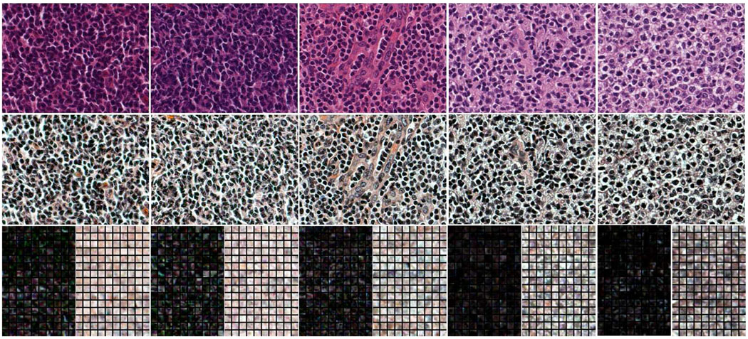
Due to the non-uniform staining, and especially, the varying contrast between the nuclei and extra-cellular regions accross different sections (caused by inconsistent illumination), histopathological images usually exhibit non-consistent colors (e.g., see the five training images in the first row of Fig.1). Therefore, it is desirable to normalize the contrast across different section images. To do this, we transform the original section images by applying histogram equalization to each channel of the RGB color space. The second row corresponds to the transformed training images, which show more consistent lighting conditions across different section images than the original ones. From each of the five transformed images, we manually mark 150 locations in the nuclei and extracellular regions, respectively. An 11 × 11 local neighborhood at each marked location is cropped as a training image patch. Therefore, a total of 750 positive (corresponding to nuclei regions) and 750 negative (corresponding to extra-cellular regions) training patches are created. The third column of Fig.1 shows these patches (darker corresponding to positive and lighter corresponding to negative).

Fig. 1.

First row: five original training images. Second row: training images after histogram equalization. Third row: 150 small positive (darker) and 150 negative (lighter) image patches extracted from the nuclear and extra-cellular regions of each training image, respectively.

B. Extraction of LFT RGB-color feature from an image patch

Let x_a(t) be a continuous time function with period T. The x_a(t) is discretized into series x(n) by taking N samples T/N apart. So x(n) has period of length N. The pair of Fourier transform of x(n) is

$$\mathrm{X}(k)=\text{DFT}[\mathrm{x}(n)]=\frac{1}{N}{\displaystyle \sum _{n=0}^{N-1}}\mathrm{x}(n)e^{-j(\frac{2\pi }{N})\mathit{\text{kn}}}$$ (3)

$$\mathrm{x}(n)=\text{iDFT}[\mathrm{X}(k)]={\displaystyle \sum _{n=0}^{N-1}}\mathrm{X}(k)e^{j(\frac{2\pi }{N})\mathit{\text{kn}}}$$ (4)

where DFT[·]and iDFT[·] represents the discrete Fourier transform and inverse discrete Fourier transform, respectively.

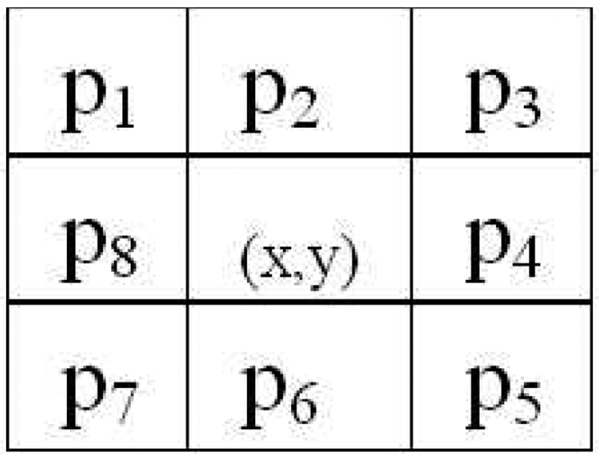
For an image patch, its LFT color feature is extracted from RGB channels, respectively. In the following, we only introduce the LFT feature extraction process from a single channel (e.g., R-channel). Let I(x, y) denote the pixel of the grey-tone (i.e., single-channel) image patch I_h×w at (x, y), where h and w correspond to the height and width of I_h×w. The 8-neighbor pixels of I(x, y) are illustrated as Fig.2. The discrete Fourier transform (DFT) of the 8-pixel sequence p₁ through p₈ is computed based on Eq.3 for each pixel of I_h×w. Therefore we can get eight local Fourier transform (LFT) maps [6], denoted by L_i, i = 1, 2, …, 8. The first-order moment, i.e., the mean value, of each LFT map (excluding border pixels which are invalid due to the LFT operation) is used for a more compact representation. Therefore, an 8-dimensional feature vector can be extracted from a single color channel. Repeating the above process to each channel independently, an 8 × 3 LFT feature matrix, which encodes both color and texture, can be extracted from a color image patch.

Fig. 2.

The eight neighbors of the image pixel at (x, y).

We might extract the LFT feature for each training image patch by applying the above process in RGB channels, and the LFT feature is denoted by Q_ij, where i = 1, 2 is the index of class (cell-nuclei and extra-cellular regions) and j = 1, …, N_i (N_i is the number of image patches of class i) is the index of image patch within each class. Let c be the number of classes (c = 2 in this paper), and $N_t={\displaystyle {\sum }_{i=1}^c{N}_i}$ be the total number of training image patches. The intra- and inter-class covariance matrices of Q_ij are constructed as

$${\mathbf{S}}_b=\frac{1}{c}{\displaystyle \sum _{i=1}^c}({\mathbf{M}}_i-\mathbf{M}){({\mathbf{M}}_i-\mathbf{M})}^T$$ (5)

$${\mathbf{S}}_w=\frac{1}{N_t}{\displaystyle \sum _{i=1}^c}{\displaystyle \sum _{j=1}^{N_i}}({\mathbf{Q}}_{\mathit{\text{ij}}}-{\mathbf{M}}_i){({\mathbf{Q}}_{\mathit{\text{ij}}}-{\mathbf{M}}_i)}^T$$ (6)

where $\mathbf{M}=\frac{1}{N_t}{\displaystyle {\sum }_{i=1}^c{\displaystyle {\sum }_{j=1}^{N_i}{\mathbf{Q}}_{\mathit{\text{ij}}}}}$ is the total mean of Q_ij of all classes, and ${\mathbf{M}}_i=\frac{1}{N_i}{\displaystyle {\sum }_{j=1}^{N_i}{\mathbf{Q}}_{\mathit{\text{ij}}}}$ is the mean of Q_ij of class i.

C. Efficient LFT feature extraction

Although the computation of LFT feature from one single small image patch might take a very small amount of time, if the image to be segmented has a large size (e.g., over 2000 × 1000 for our histopathological images), it would be extremely time-consuming by using the LFT feature extraction method described in Section III-B. The reason is that, at each pixel, the segmentation algorithm needs to extract an LFT feature (in an 11 × 11 neighborhood) as input.

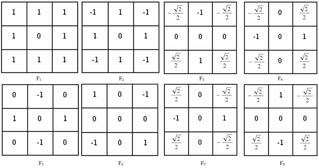
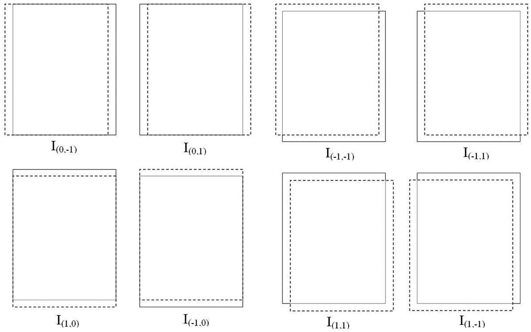
Therefore, we propose an efficient LFT extraction method in this section. We use similar notations as in Section III-B except that the image I is not limited to small image patches. Instead, we use I to represent the whole histopathological image. By re-examining the above LFT feature extraction, it can be noticed that this process is equivalent to applying eight kernels [7], F_i, to image I, where the eight kernels are shown in Fig.3. To get a fast computation for L_i, we initially make a shift of image I to eight different directions by some offset d (d = 1 for our application), where the eight directions correspond to left, right, up, down, up-left, up-right, down-left and down-right. We denote the eight shifted versions as I_0,−1, I_0,1, I_−1,0, I_1,0, I_−1,−1, I_−1,1, I_1,−1, and I_1,1, respectively (see Fig.4). Accordingly, the eight LFT maps are computed as follows (note that $\sqrt{2}/2$ is approximately 0.707):

$${\mathrm{L}}_1={\mathrm{I}}_{0,-1}+{\mathrm{I}}_{0,1}+{\mathrm{I}}_{-1,0}+{\mathrm{I}}_{1,0}+{\mathrm{I}}_{-1,-1}+{\mathrm{I}}_{-1,1}+{\mathrm{I}}_{1,-1}+{\mathrm{I}}_{1,1}$$ (7)

$${\mathrm{L}}_2=\left[{\mathrm{I}}_{0,-1}+{\mathrm{I}}_{0,1}+{\mathrm{I}}_{-1,0}+{\mathrm{I}}_{1,0}\right]-\left[{\mathrm{I}}_{-1,-1}+{\mathrm{I}}_{-1,1}+{\mathrm{I}}_{1,-1}+{\mathrm{I}}_{1,1}\right]$$ (8)

$${\mathrm{L}}_3=0.707\times \left[{\mathrm{I}}_{-1,1}+{\mathrm{I}}_{1,1}-{\mathrm{I}}_{-1,-1}-{\mathrm{I}}_{1,-1}\right]+{\mathrm{I}}_{0,1}-{\mathrm{I}}_{0,-1}$$ (9)

$${\mathrm{L}}_4=0.707\times \left[{\mathrm{I}}_{1,-1}+{\mathrm{I}}_{1,1}-{\mathrm{I}}_{-1,-1}-{\mathrm{I}}_{-1,1}\right]+{\mathrm{I}}_{1,0}-{\mathrm{I}}_{-1,0}$$ (10)

$${\mathrm{L}}_5={\mathrm{I}}_{0,-1}+{\mathrm{I}}_{0,1}-{\mathrm{I}}_{-1,0}-{\mathrm{I}}_{1,0}$$ (11)

$${\mathrm{L}}_6={\mathrm{I}}_{-1,-1}+{\mathrm{I}}_{1,1}-{\mathrm{I}}_{-1,1}-{\mathrm{I}}_{1,-1}$$ (12)

$${\mathrm{L}}_7=0.707\times \left[{\mathrm{I}}_{-1,-1}+{\mathrm{I}}_{1,-1}-{\mathrm{I}}_{-1,1}-{\mathrm{I}}_{1,1}\right]+{\mathrm{I}}_{0,1}-{\mathrm{I}}_{0,-1}$$ (13)

$${\mathrm{L}}_8=0.707\times \left[{\mathrm{I}}_{1,-1}+{\mathrm{I}}_{1,1}-{\mathrm{I}}_{-1,-1}-{\mathrm{I}}_{-1,1}\right]+{\mathrm{I}}_{-1,0}-{\mathrm{I}}_{1,0}$$ (14)

Fig. 3.

The eight kernels for computing LFT maps.

Fig. 4.

The eight shifted versions of image I.

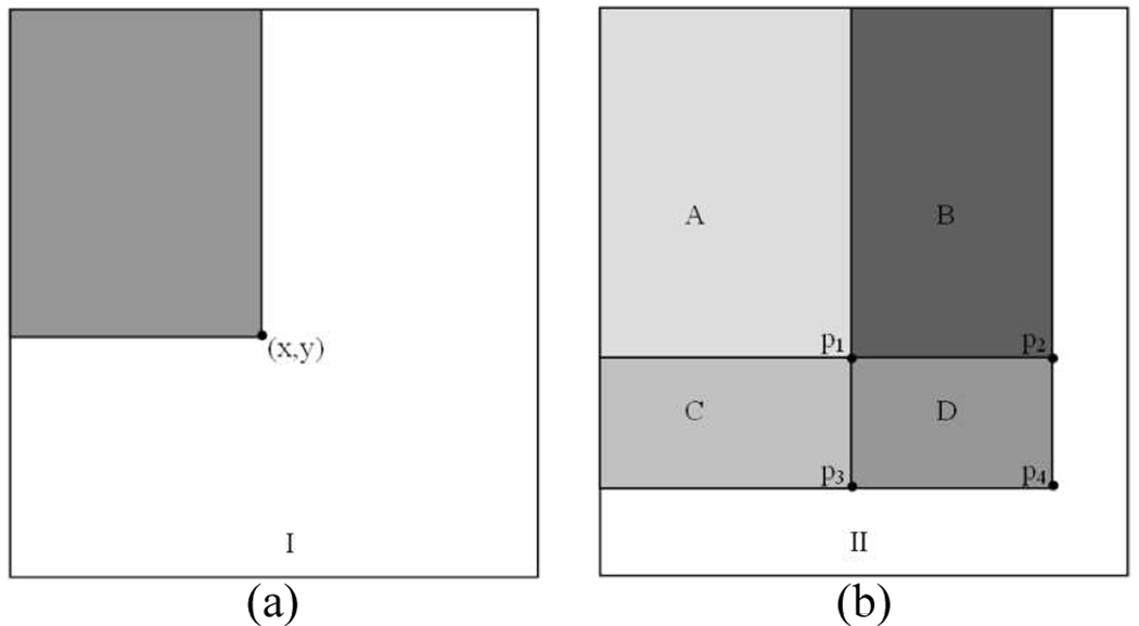
To efficiently compute the LFT feature at any pixel location from the above LFT maps, we use an intermediate representation for each LFT map, i.e., the integral map. The integral map (or integral image) technique [8] provides a very efficient way to compute the sum of an arbitrary subset of a 2D matrix. The integral map at location (x,y) contains the sum of the pixels above and to the left of (x,y), inclusive,

$$\text{II}(x,y)={\displaystyle \sum _{x\prime \le x,y\prime \le y}}\mathrm{I}(x\prime ,y\prime )$$ (15)

where II is the integral map, and I is the original 2D matrix, shown as Fig.5. Using the integral map, any rectangular sum can be computed in four array references. As illustrated in Fig.5 (b), the sum of the pixels within rectangle D can be computed with four array references. The value of the integral map at location p₁ is the sum of the pixels in rectangle A. The value at location p₂ is A+B, at location p₃ is A+C, at location p₄ is A+B+C+D. The sum within D can be computed as II(p₄) + II(p₁) − II(p₂) − II(p₃).

Fig. 5.

Illustration of computing the sum of a subset of a 2D matrix efficiently by using the integral map. (a): the original image. (b): the integral image.

We construct an integral map representation for each LFT map, and we denote these eight integral maps by iL_t, t = 1,2, …, 8. Since, for a given pixel, the LFT feature extracted from its local neighborhood consists of the first-order moments (mean) of the LFT maps. Using iL_t, the mean can be efficiently retrieved by referencing four array entries and multiplying one factor.

By assuming that the complexity of multiplication is t times that of addition, theoretically, we can approximately achieve $\frac{7744t+968}{4t+104}$ (e.g., 147 if let t be 2 with new processor architecture) times faster than brute-force one (see the complexity analysis in the appendix section).

D. Construction of covariance matrices in MDC space

In the above section, the LFT features are extracted in RGB space. However, these LFT feature vectors might not be optimal in terms of discrimination of nuclei from extra-cellular region. Therefore, the purpose of this and next sections is to learn the most discriminant color space, MDC, from which the extracted LFT features have more discriminative power.

The learning of MDC space (or the coefficient matrix A) is based on the Fisher-Rao discriminant analysis [14], for which the intra- and inter-class covariance matrices of the LFT features need to be constructed in MDC space. To this end, we assume A in Eq.1 is known so that we can transform the images from RGB to MDC space. Thanks to the linear nature of Eq.1, the efficient LFT feature extraction method proposed in Section III-C can also be applied to the MDC channels. Let I and Ĩ be the whole image represented in RGB and MDC space, respectively. Correspondingly, let Ĩ_0,−1, Ĩ_0,1, Ĩ_−1,0, Ĩ_1,0, Ĩ_−1,−1, Ĩ_−1,1, Ĩ_1,−1 and Ĩ_1,1 be the shifted versions of Ĩ. Similar to L_i (from Eq.7 to Eq.14), let L̃_i, i = 1, …, 8 be the LFT maps obtained from Ĩ_0,−1, Ĩ_0,1, Ĩ_−1,0, Ĩ_1,0, Ĩ_−1,−1, Ĩ_−1,1, Ĩ_1,−1 and Ĩ_1,1. Obviously, Ĩ_0,−1 = I_0,−1 × A, Ĩ_0,1 = I_0,1 × A, Ĩ_−1,0 = I_−1,0 × A, Ĩ_1,0 = I_1,0 × A, Ĩ_−1,−1 = I_−1,−1 × A, Ĩ_−1,1 = I_−1,1 × A, Ĩ_1,−1 = I_1,−1 × A and Ĩ_1,1 = I_1,1 × A. Therefore, we can easily obtain the following equation,

$${\tilde{\mathrm{L}}}_i={\mathrm{L}}_i\times \mathrm{A},i=1,\dots ,8$$ (16)

and

$$\mathrm{i}{\tilde{\mathrm{L}}}_i={\text{iL}}_i\times \mathrm{A},i=1,\dots ,8$$ (17)

where iL̃_i is the integral map of L̃_i.

Likewise, the LFT feature extracted from MDC channels at the local neighborhood of a given pixel, denoted as Q̃. It is straightforward to see that

$$\tilde{\mathrm{Q}}=\mathrm{Q}\times \mathrm{A}$$ (18)

Similarly, the LFT feature matrices can be extracted for each training image patch from the MDC channels, which are denoted by Q̃_ij. Thereafter, we create the intra- and inter-covariance matrices of Q̃_ij as follows,

$$\begin{array}{cc}{\tilde{\mathbf{S}}}_b\hfill & =\frac{1}{c}{\displaystyle \sum _{i=1}^c}({\tilde{\mathbf{M}}}_i-\tilde{\mathbf{M}}){({\tilde{\mathbf{M}}}_i-\tilde{\mathbf{M}})}^T\hfill \\ \hfill & =\frac{1}{c}{\displaystyle \sum _{i=1}^c}({\mathbf{M}}_i-\mathbf{M}){\mathbf{\text{AA}}}^T{({\mathbf{M}}_i-\mathbf{M})}^T\hfill \end{array}$$ (19)

$$\begin{array}{cc}{\tilde{\mathbf{S}}}_w\hfill & =\frac{1}{N_t}{\displaystyle \sum _{i=1}^c}{\displaystyle \sum _{j=1}^{N_i}}({\tilde{\mathbf{Q}}}_{\mathit{\text{ij}}}-{\tilde{\mathbf{M}}}_i){({\tilde{\mathbf{Q}}}_{\mathit{\text{ij}}}-{\tilde{\mathbf{M}}}_i)}^T\hfill \\ \hfill & =\frac{1}{N_t}{\displaystyle \sum _{i=1}^c}{\displaystyle \sum _{j=1}^{N_i}}({\mathbf{Q}}_{\mathit{\text{ij}}}-{\mathbf{M}}_i){\mathbf{\text{AA}}}^T{({\mathbf{Q}}_{\mathit{\text{ij}}}-{\mathbf{M}}_i)}^T\hfill \end{array}$$ (20)

where $\tilde{\mathbf{M}}=\frac{1}{N_t}{\displaystyle {\sum }_{i=1}^c{\displaystyle {\sum }_{j=1}^{N_i}{\tilde{\mathbf{Q}}}_{\mathit{\text{ij}}}}}$ is the total mean of the Q̃_ij of all classes, and ${\tilde{\mathbf{M}}}_i=\frac{1}{N_i}{\displaystyle {\sum }_{j=1}^{N_i}{\tilde{\mathbf{Q}}}_{\mathit{\text{ij}}}}$ is the mean of Q̃_ij of class i.

Rewriting Eq.19 and Eq.20, S̃_b and S̃_w can also be represented by

$${\tilde{\mathbf{S}}}_b=\frac{1}{c}{\mathbf{\Phi }}_{\mathit{\text{sb}}}{\mathbf{\Delta }}_{\mathit{\text{sb}}}{\mathbf{\Delta }}_{\mathit{\text{sb}}}^T{\mathbf{\Phi }}_{\mathit{\text{sb}}}^T$$

and

$${\tilde{\mathbf{S}}}_w=\frac{1}{N_t}{\mathbf{\Phi }}_{\mathit{\text{sw}}}{\mathbf{\Delta }}_{\mathit{\text{sw}}}{\mathbf{\Delta }}_{\mathit{\text{sw}}}^T{\mathbf{\Phi }}_{\mathit{\text{sw}}}^T$$

where,

$${\mathbf{\Phi }}_{\mathit{\text{sb}}}=[({\mathbf{M}}_1-\mathbf{M}),\dots ,({\mathbf{M}}_c-\mathbf{M})]$$

and

$${\mathbf{\Phi }}_{\mathit{\text{sw}}}=[({\mathbf{Q}}_{11}-{\mathbf{M}}_1),\dots ,({\mathbf{Q}}_{{\mathit{\text{cN}}}_c}-{\mathbf{M}}_c)]$$

The Δ_sb and Δ_sw take the following form,

$$\begin{array}{c}{\mathbf{\Delta }}_{\mathit{\text{sb}}}={\left(\begin{array}{cc}\mathbf{A}& \mathbf{0}\\ \mathbf{0}& \mathbf{A}\end{array}\right)}_{(3\times c)\times (3\times c)}\\ {\mathbf{\Delta }}_{\mathit{\text{sw}}}={\left(\begin{array}{cccc}\mathbf{A}& \mathbf{0}& \cdots & \mathbf{0}\\ \mathbf{0}& \mathbf{A}& \cdots & \mathbf{0}\\ ⋮& ⋮& \ddots & ⋮\\ \mathbf{0}& \mathbf{0}& \cdots & \mathbf{A}\end{array}\right)}_{(3{\displaystyle {\sum }_{i=1}^c}{N}_i)\times (3{\displaystyle {\sum }_{i=1}^c}{N}_i)}\end{array}$$

Based on Fisher-Rao discriminant analysis (Eq.2), the most discriminant color space, MDC, (i.e., the coefficient matrix A), can be obtained by maximizing the inter-class scatter and minimizing the intra-class scatter of Q̃_ij based on projection matrix P. By inserting the re-formulated S̃_b and S̃_w into Eq.2, we get

$$\{{\mathbf{A}}^{*},{\mathbf{P}}^{*}\}={\text{arg}}_{\mathbf{A},\mathbf{P}}\text{ max }\frac{N_t·\mathit{\text{tr}}({\mathbf{P}}^T{\mathbf{\Phi }}_{\mathit{\text{sb}}}{\mathbf{\Delta }}_{\mathit{\text{sb}}}{\mathbf{\Delta }}_{\mathit{\text{sb}}}^T{\mathbf{\Phi }}_{\mathit{\text{sb}}}^T\mathbf{P})}{c·\mathit{\text{tr}}({\mathbf{P}}^T{\mathbf{\Phi }}_{\mathit{\text{sw}}}{\mathbf{\Delta }}_{\mathit{\text{sw}}}{\mathbf{\Delta }}_{\mathit{\text{sw}}}^T{\mathbf{\Phi }}_{\mathit{\text{sw}}}^T\mathbf{P})}$$ (21)

E. Iterative Fisher-Rao optimization

To our best knowledge, there is no close-form solution for the maximization of Eq.21. Therefore, we propose to iteratively optimize it. The algorithm is listed in Table I. The basic idea is to initialize A by a 3 × 3 identity matrix. Then we get P* by solving the following well-posed generalized eigenvalue problem (step S₂, S₃ and S₄ of Table I, see Lemma 2 for proof)

$$\frac{1}{c}·({\mathbf{\Phi }}_{\mathit{\text{sb}}}{\mathbf{\Delta }}_{\mathit{\text{sb}}}{\mathbf{\Delta }}_{\mathit{\text{sb}}}^T{\mathbf{\Phi }}_{\mathit{\text{sb}}}^T)\mathbf{P}=(\frac{1}{N_t}·{\mathbf{\Phi }}_{\mathit{\text{sw}}}{\mathbf{\Delta }}_{\mathit{\text{sw}}}{\mathbf{\Delta }}_{\mathit{\text{sw}}}^T{\mathbf{\Phi }}_{\mathit{\text{sw}}}^T)\mathbf{P}\mathrm{\Lambda }$$

TABLE I.

Iterative Fisher-Rao Optimization

S1. Let J1 = 0; J2 = 0; Initialize A by a 3×3 identity matrix.

S2. Construct Δsb and Δsw using A.

S3. Get ${\mathbf{P}}^{*}={\text{arg}}_{\mathbf{P}}\text{ max }\frac{N_t·\mathit{\text{tr}}({\mathbf{P}}^T{\mathbf{\Phi }}_{\mathit{\text{sb}}}{\mathbf{\Delta }}_{\mathit{\text{sb}}}{\mathbf{\Delta }}_{\mathit{\text{sb}}}^T{\mathbf{\Phi }}_{\mathit{\text{sb}}}^T\mathbf{P})}{c·\mathit{\text{tr}}({\mathbf{P}}^T{\mathbf{\Phi }}_{\mathit{\text{sw}}}{\mathbf{\Delta }}_{\mathit{\text{sw}}}{\mathbf{\Delta }}_{\mathit{\text{sw}}}^T{\mathbf{\Phi }}_{\mathit{\text{sw}}}^T\mathbf{P})}$ by solving the generalized eigenvalue problem $\frac{1}{c}\left({\mathbf{\Phi }}_{\mathit{\text{sb}}}{\mathbf{\Delta }}_{\mathit{\text{sb}}}{\mathbf{\Delta }}_{\mathit{\text{sb}}}^T{\mathbf{\Phi }}_{\mathit{\text{sb}}}^T\right)\mathbf{P}=\frac{1}{N_t}\left({\mathbf{\Phi }}_{\mathit{\text{sw}}}{\mathbf{\Delta }}_{\mathit{\text{sw}}}{\mathbf{\Delta }}_{\mathit{\text{sw}}}^T{\mathbf{\Phi }}_{\mathit{\text{sw}}}^T\right)\mathbf{P}\mathrm{\Lambda }$, where P* consists of the three eigenvectors which corresponds to the three largest eigenvalues (See Lemma 2)

S4. Compute $J_2=\frac{N_t·\mathit{\text{tr}}({({\mathbf{P}}^{*})}^T{\mathbf{\Phi }}_{\mathit{\text{sb}}}{\mathbf{\Delta }}_{\mathit{\text{sb}}}{\mathbf{\Delta }}_{\mathit{\text{sb}}}^T{\mathbf{\Phi }}_{\mathit{\text{sb}}}^T{\mathbf{P}}^{*})}{c·\mathit{\text{tr}}({({\mathbf{P}}^{*})}^T{\mathbf{\Phi }}_{\mathit{\text{sw}}}{\mathbf{\Delta }}_{\mathit{\text{sw}}}{\mathbf{\Delta }}_{\mathit{\text{sw}}}^T{\mathbf{\Phi }}_{\mathit{\text{sw}}}^T{\mathbf{P}}^{*})}$.

S5. While J2 − J1 > t

S6. J1 ← J2. P ← P*

S7. Construct ϒsb and ϒsw using P.

S8. Get ${\mathbf{A}}^{*}={\text{arg}}_{\mathbf{A}}\text{ max }\frac{\mathit{\text{tr}}({\mathbf{A}}^T{\mathbf{\Phi }}_{\mathit{\text{sb}}}^T{\mathbf{\Upsilon }}_{\mathit{\text{sb}}}{\mathbf{\Upsilon }}_{\mathit{\text{sb}}}^T{\mathbf{\Phi }}_{\mathit{\text{sb}}}\mathbf{A})}{\mathit{\text{tr}}({\mathbf{A}}^T{\mathbf{\Phi }}_{\mathit{\text{sw}}}^T{\mathbf{\Upsilon }}_{\mathit{\text{sw}}}{\mathbf{\Upsilon }}_{\mathit{\text{sw}}}^T{\mathbf{\Phi }}_{\mathit{\text{sw}}}\mathbf{A})}$ by solving the $\left({\mathbf{\Phi }}_{\mathit{\text{sb}}}^T{\mathbf{\Upsilon }}_{\mathit{\text{sb}}}{\mathbf{\Upsilon }}_{\mathit{\text{sb}}}^T{\mathbf{\Phi }}_{\mathit{\text{sb}}}\right)\mathbf{A}=\left({\mathbf{\Phi }}_{\mathit{\text{sw}}}^T{\mathbf{\Upsilon }}_{\mathit{\text{sw}}}{\mathbf{\Upsilon }}_{\mathit{\text{sw}}}^T{\mathbf{\Phi }}_{\mathit{\text{sw}}}\right)\mathbf{A}\mathrm{\Lambda }$

S9. A ← A*

S10. Get P* and J2 by repeating steps S2, S3 and S4.

S11. End While

Due to the fact that tr(A + B) = tr(A) + tr(B) and tr(AB) = tr(BA) for any two matrix A and B, we can readily see that the maximization of the following two equations is equivalent.

$$\begin{array}{c}J=\frac{N_t·\mathit{\text{tr}}({\mathbf{P}}^T({\displaystyle {\sum }_{i=1}^c}({\mathbf{M}}_i-\mathbf{M}){\mathbf{\text{AA}}}^T{({\mathbf{M}}_i-\mathbf{M})}^T)\mathbf{P})}{c·\mathit{\text{tr}}({\mathbf{P}}^T({\displaystyle {\sum }_{i=1}^c}{\displaystyle {\sum }_{j=1}^{N_i}}({\mathbf{Q}}_{\mathit{\text{ij}}}-{\mathbf{M}}_i){\mathbf{\text{AA}}}^T{({\mathbf{Q}}_{\mathit{\text{ij}}}-{\mathbf{M}}_i)}^T)\mathbf{P})}\hfill \\ J=\frac{N_t·\mathit{\text{tr}}({\mathbf{A}}^T({\displaystyle {\sum }_{i=1}^c}{({\mathbf{M}}_i-\mathbf{M})}^T{\mathbf{\text{PP}}}^T({\mathbf{M}}_i-\mathbf{M}))\mathbf{A})}{c·\mathit{\text{tr}}({\mathbf{A}}^T({\displaystyle {\sum }_{i=1}^c}{\displaystyle {\sum }_{j=1}^{N_i}}{({\mathbf{Q}}_{\mathit{\text{ij}}}-{\mathbf{M}}_i)}^T{\mathbf{\text{PP}}}^T({\mathbf{Q}}_{\mathit{\text{ij}}}-{\mathbf{M}}_i))\mathbf{A})}\hfill \end{array}$$

Therefore, inserting P = P*, we get A* by solving the following well-posed eigenvalue problem (step S₈ of Table I)

$$\frac{1}{c}({\mathbf{\Phi }}_{\mathit{\text{sb}}}^T{\mathbf{\Upsilon }}_{\mathit{\text{sb}}}{\mathbf{\Upsilon }}_{\mathit{\text{sb}}}^T{\mathbf{\Phi }}_{\mathit{\text{sb}}})\mathbf{A}=\frac{1}{N_t}({\mathbf{\Phi }}_{\mathit{\text{sw}}}^T{\mathbf{\Upsilon }}_{\mathit{\text{sw}}}{\mathbf{\Upsilon }}_{\mathit{\text{sw}}}^T{\mathbf{\Phi }}_{\mathit{\text{sw}}})\mathbf{A}\mathrm{\Lambda }$$

where,

$$\begin{array}{c}{\mathbf{\Upsilon }}_{\mathit{\text{sb}}}={\left(\begin{array}{cc}\mathbf{P}& \mathbf{0}\\ \mathbf{0}& \mathbf{P}\end{array}\right)}_{(8\times c)\times (3\times c)}\\ {\mathbf{\Upsilon }}_{\mathit{\text{sw}}}={\left(\begin{array}{cccc}\mathbf{P}& \mathbf{0}& \cdots & \mathbf{0}\\ \mathbf{0}& \mathbf{P}& \cdots & \mathbf{0}\\ ⋮& ⋮& \ddots & ⋮\\ \mathbf{0}& \mathbf{0}& \cdots & \mathbf{P}\end{array}\right)}_{(8{\displaystyle {\sum }_{i=1}^c}{N}_i)\times (3{\displaystyle {\sum }_{i=1}^c}{N}_i)}\end{array}$$

The ratio of inter-class scatter to intra-class scatter is computed as $J=\frac{N_t·\mathit{\text{tr}}\left({({\mathbf{P}}^{*})}^T({\displaystyle {\sum }_{i=1}^c({\mathbf{M}}_i-\mathbf{M}){\mathbf{A}}^{*}{({\mathbf{A}}^{*})}^T{({\mathbf{M}}_i-\mathbf{M})}^T}){\mathbf{P}}^{*}\right)}{c·\mathit{\text{tr}}\left({({\mathbf{P}}^{*})}^T({\displaystyle {\sum }_{i=1}^c{\displaystyle {\sum }_{j=1}^{N_i}({\mathbf{Q}}_{\mathit{\text{ij}}}-{\mathbf{M}}_i){\mathbf{A}}^{*}{({\mathbf{A}}^{*})}^T{({\mathbf{Q}}_{\mathit{\text{ij}}}-{\mathbf{M}}_i)}^T}}){\mathbf{P}}^{*}\right)}$ This process proceeds iteratively until J converges to a local maximum value.

Lemma 1: The row vectors of Φ_sw (or Φ̃_sw) are linearly independent. See proof in Appendix.

Lemma 2: The $({\mathbf{\Phi }}_{\mathit{\text{sb}}}{\mathbf{\Delta }}_{\mathit{\text{sb}}}{\mathbf{\Delta }}_{\mathit{\text{sb}}}^T{\mathbf{\Phi }}_{\mathit{\text{sb}}}^T)\mathbf{P}=({\mathbf{\Phi }}_{\mathit{\text{sw}}}{\mathbf{\Delta }}_{\mathit{\text{sw}}}{\mathbf{\Delta }}_{\mathit{\text{sw}}}^T{\mathbf{\Phi }}_{\mathit{\text{sw}}}^T)\mathbf{P}\mathrm{\Lambda }$ is a well-posed generalized eigenvalue problem (S₃ of Table I). See proof in Appendix.

Note that the $({\mathbf{\Phi }}_{\mathit{\text{sb}}}^T{\mathbf{\Upsilon }}_{\mathit{\text{sb}}}{\mathbf{\Upsilon }}_{\mathit{\text{sb}}}^T{\mathbf{\Phi }}_{\mathit{\text{sb}}})\mathbf{A}=({\mathbf{\Phi }}_{\mathit{\text{sw}}}^T{\mathbf{\Upsilon }}_{\mathit{\text{sw}}}{\mathbf{\Upsilon }}_{\mathit{\text{sw}}}^T{\mathbf{\Phi }}_{\mathit{\text{sw}}})\mathbf{A}\mathrm{\Lambda }$ is also a well-posed generalized eigenvalue problem (S₈ of Table I). This is due to the fact that ${\mathbf{\Phi }}_{\mathit{\text{sw}}}^T{\mathbf{\Upsilon }}_{\mathit{\text{sw}}}{\mathbf{\Upsilon }}_{\mathit{\text{sw}}}^T{\mathbf{\Phi }}_{\mathit{\text{sw}}}$ is full rank (proof similar to the one for Lemma 2).

F. Learned color space and segmentation via classification

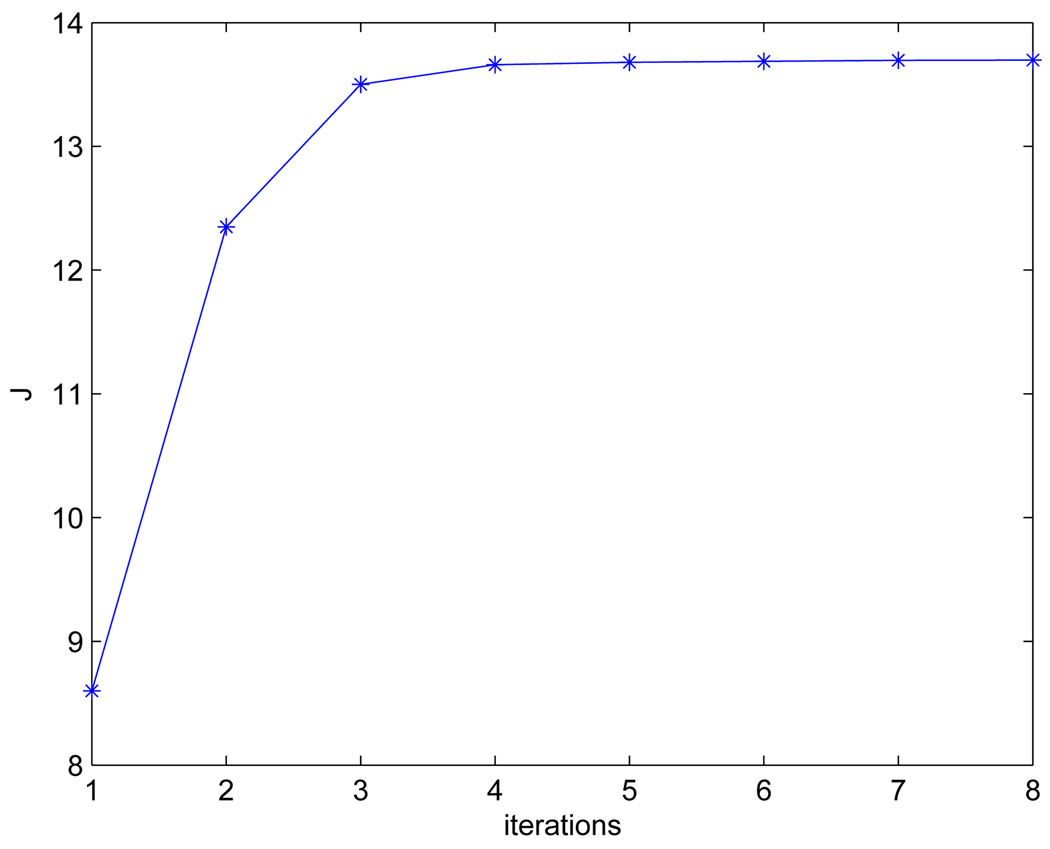
By the iterative optimization, the learned optimal A, A*, for the MDC color channels are [−0.8251.311.03; −0.2680.168 − 2.165; 0.017 − 1.6001.084]. We set t to 0.001 (S₅ of Table I), which makes the algorithm converge within 8 iterations (see Fig.7). The learned MDC color space achieves more discriminative power than RGB space in terms of the obtained optimal J*, where J* = 13.7 in MDC space and J* = 4.5 in RGB space.

Fig. 7.

Convergence of J within eight iterations by setting t to 0.001.

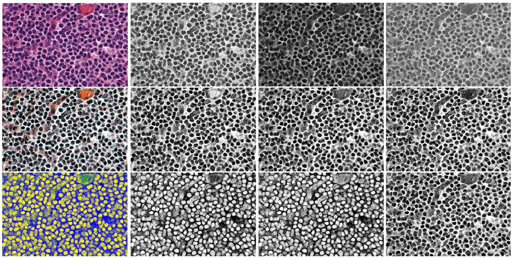
Based on the learned A*, the histogram-equalized RGB image is transformed to the new MDC color space. Fig.6 shows one example image which is subject to the color transformation based on A*.

Fig. 6.

First row: RGB channels. Second row: RGB channels after histogram equalization. Third row: MDC channels

Before segmentation, the background (white region) and red-blood cells (red region) are pre-segmented in an heuristical thresholding way in RGB channels. The segmentation is performed in the MDC channels, where, for each pixel of the remaining area, an 8×3 LFT feature matrix is extracted from its 11×11 local neighborhood (based on the proposed efficient method in Section III-C). Then the LFT feature is projected by the learned P* to get a more compact 3×3 LFT feature matrix.

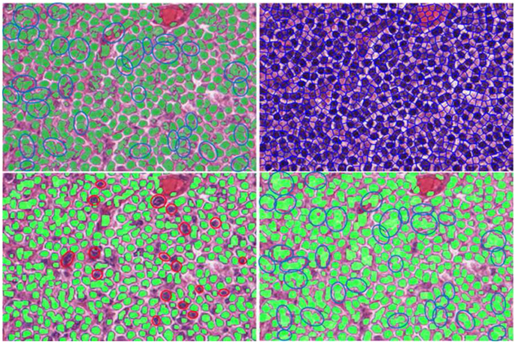
In a similar way, a 3×3 LFT feature matrix is extracted from the MDC channels for each training image patch. Therefore, a total number of 750 such LFT feature matrices are extracted for each class. K-means clustering is applied to these feature matrices to get a more compact representation of each class (each class is represented by 20 cluster centers). In segmentation of a given image, the 3×3 LFT feature extracted at each pixel is compared with those of two classes (40 cluster centers), K-NN classifier (K=9 in this paper) is used to determine the pixel’s class label. Fig.8 shows an example segmentation result by the proposed algorithm and comparison with Superpixel [9] and GraphCut [10] algorithms, where the top left one is the result of the proposed segmentation method, the top right one corresponding to Superpixel result. The bottom two are the results by GraphCut (the left set to two clusters and the right to three clusters). The result of our algorithm looks much better than those of Superpixel and GraphCut in terms of the number of touching cells and segmentation accuracy. For example, the red elliptical areas are wrong segmentations by GraphCut (with two clusters). The blue elliptical areas show the touching cells that exist in GraphCut segmentation (with three clusters) while they do not exist in our segmentation (our result shows much fewer touching cells than GraphCut). More evaluation on the proposed segmentation method and comparison with the Graph-cut, Mean-shift, Superpixel and two cell image segmentation algorithms will be given in Section V.

Fig. 8.

Top left: our segmentation result. Top right: result by Superpixel. The bottom two images are the results by GraphCut (the left set to two clusters and the right to three clusters)

IV. TOUCHING-CELL SPLITTING

The color segmentation algorithm given in the above section can separate the nuclear regions from the extracellular and background areas, and results in a binary foreground/background complex structures, which can be rather far away from a final quantification of features of single cells since cells may overlap and cluster strongly. Separating partially or totally fused entities like cells is a problem which cannot be solved completely by a single watershed segmentation [27], [28] or basic morphological operations of images. In this section, we propose an iterative algorithm to split touching cells based on radial-symmetry interest point [40] and concavity detection. Before giving details of our algorithm, we briefly review some related works in touching-cell splitting.

Generally, the watershed algorithms [27], [28] are probably the most widely used touching-cell splitting schemes. Recently, it has been improved by marker-controlled methods such as h-minima [41]. Mao et al. propose to use both grayscale and complimented distance images for marker detection by assuming that the intra-nuclei region is homogeneous while inter-nuclei region has more variations in pixel intensity [36]. Cheng and Rajapakse apply active contour algorithm to separate the cells from background before proposing to use an adaptive H-minima transform to extract shape markers [42]. Schmitt and Hasse propose to detect the radial symmetry points by iterative voting kernel approach, and use these radial symmetry points as the markers of the watershed segmentation [43]. Note that Keenan et al. also proposed an iterative touching-cell splitting method [44]. The difference between [44] and ours is that we use morphological features (such as the distance between the geometric center and the radial-symmetry point), while [44] used intensity values of pixels as the major feature. In addition, concave points [45], ellipse/curve fitting [46], and graph-cut algorithm [13] have also been widely used for touching-cell splitting.

A. Differentiation of touching cells from the non-touching ones

Different from previous cell splitting work where the touching and non-touching cells are treated equally [36], [43], we differentiate the touching cells from the non-touching ones so that our cell-splitting algorithm is only applied to the touching cells. Given a certain connected region, 𝒳_i, of the segmentation image, we use two variables to decide whether it is a single cell or a clump of touching cells: (1) by applying the radial symmetry point detector [40] to 𝒳_i, one can find the most likely radial symmetry center r_i. Let g_i denote the geometrical center of 𝒳_i. In [40], each pixel in the image votes for symmetry at a given radius based on the orientation of the pixel’s gradient. A vote is made for bright symmetrical forms on a dark background at p−, and the reverse, p+. Doing this for all pixels in the image gives the symmetry transform of the image. The r_i can be found as the corresponding pixel with maximum value in the symmetry transform image. We let

$${\varphi }_1=\{\begin{array}{cc}1\hfill & \text{if }|r_i-g_i|>{\mathrm{\gamma }}_1\hfill \\ 0\hfill & \text{otherwise}\hfill \end{array}$$ (22)

(2) We denote the area of the convex hull of 𝒳_i by 𝒜_υ and the area of 𝒳_i by 𝒜_c and we let,

$${\varphi }_2=\{\begin{array}{cc}1\hfill & \text{if }\frac{{𝒜}_c}{{𝒜}_{\upsilon }}<{\mathrm{\gamma }}_2\hfill \\ 0\hfill & \text{otherwise}\hfill \end{array}$$ (23)

where γ₁ is a threshold of the distance between the radial-symmetry center and geometrical center of 𝒳_i. The γ₂ is a threshold of the ratio of 𝒜_c to 𝒜_υ In practice, we set γ₁ to 5 pixels and γ₂ to 0.88 after tuning on some training data.

The 𝒳_i is deemed as a touching-cell clump if ϕ₁ and ϕ₂ satisfy the following condition,

$${𝒳}_i=\{\begin{array}{cc}\text{touching-cell clump}\hfill & \text{if}{\varphi }_1=1\text{ or }{\varphi }_2=1\hfill \\ \text{non-touching cell}\hfill & \text{otherwise}\hfill \end{array}$$ (24)

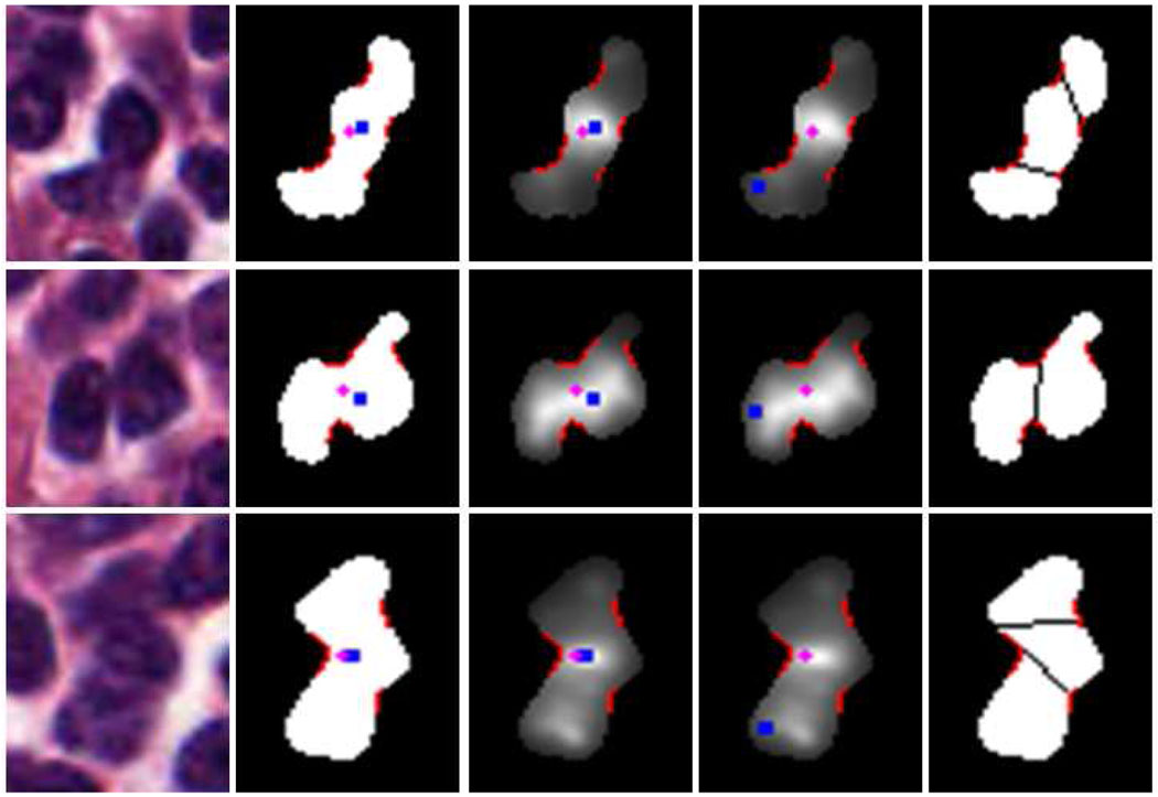
Eq. 24 means that 𝒳_i is a touching-cell clump as long as it satisfies either of the two conditions: the distance between r_i and g_i is larger than 5 or the ratio of 𝒜_c to 𝒜_υ is smaller than 0.88. However, if 𝒳_i only satisfies the later condition, its r_i is enforced to be reallocated so that r_i is far from its g_i (the reallocation of r_i is for the purpose of the splitting step, see Section IV-D). The reallocated r_i is searched ε pixels away from g_i, and ε is set to two fifths of the distance between two most apart boundary points. As an example, the second and third images of Fig.9 show the separated non-touching and touching cells, respectively. In Fig.10, each row shows the reallocated radial-symmetry point of 𝒳_i.

Fig. 9.

First image: segmentation map. Second image: non-touching cells (purple dot corresponding to the geometrical center of each connected region while yellow dot corresponding to the most likely radial symmetry center). Third image: touching cells. Fourth image: touching cells after applying Fourier shape descriptor (only using the first 12 harmonic components for this example).

Fig. 10.

First column: color image. Second column: 𝒳_i overlaid with r_i (blue dot), g_i (purple dot) and concave regions (red boundary part, see the concave region detection in Section IV-C). Third column: radial-symmetry map overlaid with r_i, g_i and concave regions. Four column: re-allocated r_i. Fifth column: splitting (see the splitting part in Section IV-D).

B. Smoothing cell boundaries by Fourier shape descriptors

We assume that cells generally have elliptical shapes. Although cells have smoother boundaries, the images obtained from previous segmentation step are often characterized by irregular and undulated contours as shown in the first image of Fig.9. To reduce those irregularities, we use Fourier shape descriptors to smooth out the boundaries of the segmented regions [47]. Fourier descriptors provide a powerful mathematical framework to reduce the irregularities of shape boundaries by eliminating high order frequencies, which usually are representative of those irregularities. The fourth image of Fig.9 shows an example of Fourier shape smoothing of the touching cells (the first 12 harmonic components are retained for smoothing).

C. Concave point detection via dominant concave region detection

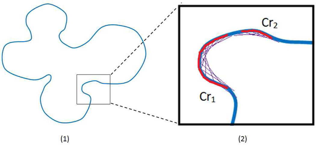
In the previous concave-point cell-splitting algorithms, angles and curvature are probably the most widely used features for concavity detection. However, both angle and curvature are vulnerable to noise, especially when the cell segmentation step cannot produce a neat and clean cell contour due to the complex background and non-uniform extra-cellular regions of the cell image. For simplicity and robustness, instead of just locating the single concave points, we propose to find the most likely concave points via detecting the dominant concave regions. Specifically, let ℒ_i be the contour of the i-th touching-cell clump after Fourier shape smoothing. Let p_j represent a point on ℒ_i, correspondingly, p_j+h and p_j−h representing the contour points which are h-point (h is set to 12) ahead and behind of p_j, respectively. If more than 60% of the line $\overline{p_{j+h}{p}_{j-h}}$, which links p_j+h and p_j−h, is outside of the clump, p_j is deemed as a concave point. In an iterative way, the concave regions on ℒ_i can be detected (e.g., see the two red detected concave regions Cr₁ and Cr₂ in Fig.11). To avoid the discontinuity in one concave region caused by noise, the adjacent fragments/points whose manifold distance (along the cell boundary) in between is less than a certain value (ξ=6) should belong to the same concave region and, therefore, are connected. To improve robustness, we only keep the dominant concave regions by discarding the trivial ones that only include three or fewer points. The most likely concave points are found as the midpoints of corresponding concave regions. Note that although certain parameters are set to work for follicular lymphoma images, the proposed approach is general and can be used for other applications with a different set of parameters.

Fig. 11.

Illustration of concave point detection via dominant concave region detection.

D. Iterative cell-clump splitting

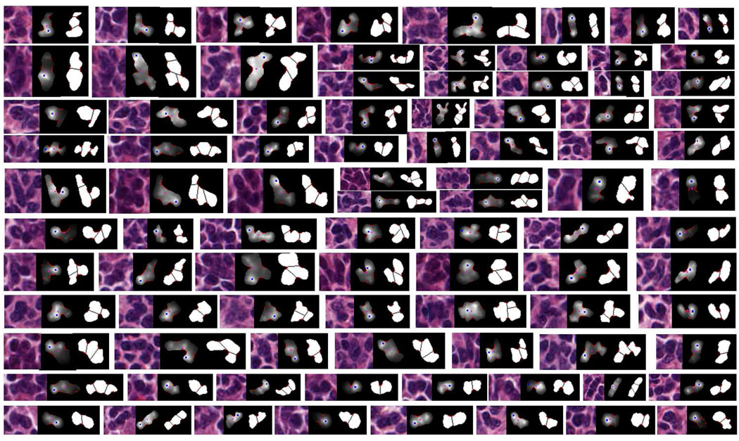
For each clump of smoothed touching cells 𝒳_i, we propose an iterative splitting algorithm where initially the two most likely concave points, which are on either side of the line linking g_i and r_i (see Section IV-A for definition), and also closest to r_i, are found and used for splitting the whole clump (the touching-cell clump is split into two by cutting along the two detected concave points). Iteratively, we apply the same splitting steps to each of the separated parts until its size is small enough (smaller than a threshold 𝒯_a¹) or it satisfies the non-touching cell condition in Eq.24. Note that the proposed splitting algorithm is much similar to a peeling process where the outermost cells are separated from the main body of cell clump before splitting the innermost cells (recall that, in the touching-cell clump, the most likely radial symmetry point should be far away from the geometrical center of the cell clump based on our touching/non-touching cell differentiation process). The iterative touching-cell splitting process is visually illustrated in Fig.12, and the whole splitting algorithm is summarized in Table II. Some representative split results are displayed in Fig.13 with one triplet for each individual clump.

Fig. 12.

Illustration of the evolving process of splitting cell clump iteratively, where one cell is separated from the clump at each step.

TABLE II.

Touching-Cell Splitting Algorithm

S1. For each connected region, 𝒳i, in the segmentation map, find the most likely radial symmetry center, ri, and its geometrical center, gi.

S2. If $\Vert r_i-g_i\Vert >5\text{ or }\frac{{𝒜}_c}{{𝒜}_{\upsilon }}<0.88$, 𝒳i is a touching-cell clump. Otherwise, 𝒳i is a non-touching cell.

S3. If 𝒳i is a touching-cell clump, its boundary is smoothed out by Fourier shape descriptor, denoted as ℒi. Otherwise, stop.

S4. For each ℒi, find its most likely concave points by detecting its dominant concave regions.

S5. Initially, the whole touching-cell clump is split into two parts by cutting along the two concave points, which are closest to ri, and are on either side of the line linking ri and gi.

S6. For each individual part, repeat a similar process as in steps S1 and S2. If it satisfies the condition for touching-cell clump in Eq.24, and its area is larger than a threshold 𝒯a, it is a touching-cell clump. Reallocate ri if necessary.

S7. If one certain part is still a touching-cell clump, repeat a similar step as in S5. Otherwise, stop.

Fig. 13.

Examples of split touching-cell clumps: for each triplet, the right image corresponds to the split result for each touching-cell clump (red boundary sections representing concave regions). The middle image corresponds to the likelihood map of radial-symmetrical point, where the blue point is the detected mostly likely radial-symmetrical point (the brighter the pixel’s intensity, the more likely the pixel is a radial symmetrical point), and the purple point is the geometrical center of the segmented clump. The left image is the original image used for producing the middle image. Note that some images have been re-scaled for better viewing.

V. EXPERIMENTAL RESULTS

We apply the proposed framework to the follicular lymphoma (FL) images, which is a cancer of lymph system and is the second most common lymphoid malignancy in the western world. The accuracy of segmentation is evaluated by comparing our results with those obtained by Graph-Cut [10], Superpixel [9], Mean-shift [11] and two state-of-the-art pathological image segmentation algorithms [12], [13] based on ground-truth segmentation². The accuracy of splitting is evaluated in terms of the number of under-splitting, over-splitting, and encroachment errors. We compared our splitting method with Al-Kofahi et al’s method [13].

A. Parameter tuning on training images

There are a few parameters that we tuned on five follicular lymphoma training images based on cross validation. Note that these training images are cropped with a size of 600×800 from each of the five training images that are shown in the first row of Fig.1 (therefore, the five cropped training images contain stained tissues which are subject to different illumination, contrast, and colors). These parameters include the window size used to define LFT features (selected as 11×11), the K value for K-NN classifier (selected as 9), the number of cluster centers in k-means algorithm (a total of 40 clusters for 2 classes), the thresholds used for the separation of touching and non-touching cells (gamma1 = 5 pixels, gamma2 = 0.88), and the parameters used in Sections IV-B and IV-C (i.e., the number of harmonics reserved for smoothing, h=12, ξ = 6, thr = 60%).

The five cropped training images are provided with ground-truth nuclei segmentation and splitting of touching-cells. For the size of the window used for LFT feature extraction, we adjusted the window size at 9×9, 11×11, 13×13, and 15×15, respectively. At the same time, we kept the other parameters unchanged. We computed the average segmentation accuracy on the five validation images, and we got the accuracy of 75.8%, 76.6%, 77.2%, and 78.5%, respectively. Although the window with the size of 15×15 gives optimal segmentation accuracy, it also produces the largest average number of touching-cell clumps after segmentation (115, 124, 144, and 157). Therefore, we choose 11×11 as the optimal window size for LFT feature extraction in terms of both segmentation accuracy and the number of produced touching-cell clumps.

For the number of clusters which are used to represent each class, we set it to 40, 30, 20, and 10, respectively, with K set to 15. Correspondingly, the segmentation accuracy is 73.2%, 74.3%, 75.5%, and 74.4%, respectively, and the number of produced touching-cell clumps is 131, 137, 128, and 129, respectively. Based on the tradeoff, we use 20 clusters in k-means to represent each class. To decide the “K” in the K-NN classifier, we adjusted it from 7 to 15 with a step of 2. The corresponding classification accuracy is 76.4%, 76.6%, 76.2%, 75.9%, and 75.6%, respectively. The number of produced touching-cell clumps is 124, 124, 125, 125, and 123, respectively. Therefore, we set K to 9.

We tune γ₁ from 4 to 9 (set γ₂ to 0.9) with a step of 1, and the number of errors in differentiation per image (on average) is 16.5, 13.4, 16.1, 17.2, 18.0. We tune γ₂ from 0.8 to 1 (keep γ₁ being 5) with a step of 0.02, and the number of differentiation errors per image (on average) is 15.5, 14.7, 13.9, 12.4, 12.7, 13.1, 13.3, 13.5, 13.9, and 14.1, respectively. Based on the differentiation error, we set γ₁ to 5 and γ₂ to 0.88. From the validation errors, we found that the performance is not sensitive to the selection of γ₁ and γ₂.

For the parameters used for dominant concave point detection, (e.g., the number of harmonics reserved for smoothing, h=12, ξ=6, etc.), we manually counted the number of dominant concave points (or the number of concave regions) for each of the touching-cell clumps. Then we applied our concave region detection algorithm to these clumps, and tune one of these parameters at a time until we get the optimal dominant concave point detection accuracy. Specifically, we found that the concave regions become flat (i.e., vanishing) if the number of harmonics set for Fourier smoothing is less than 10. Therefore, we adjusted it from 10 to 20. Based on empirically results, we found that there is no significant change in concave region detection accuracy when this number is larger than or equal to 12. The parameters h, ξ and thr were initially set based on the average number of pixels in a concave region. Then, we tuned one at a time to achieve the optimal dominant concave region detection accuracy.

B. Evaluation of segmentation accuracy

The ground-truth segmentation results are obtained manually by drawing boundaries of each cell using an in-house developed software. Typically, the size of a follicular-region image is over 2000 × 1200 whose sheer size makes the manual cell-nuclei segmentation impractical. Therefore, we have randomly cropped 21 600 × 800 images from 10 selected follicular-region images and carried out manual segmentation on these cropped images. Note that the 10 large follicular images are also selected based on the same criterion as the one to the five training images since we hope to test the robustness of our algorithm to illumination, contrast and color variations. Therefore, although the 21 test images are cropped randomly, they are not random indeed.

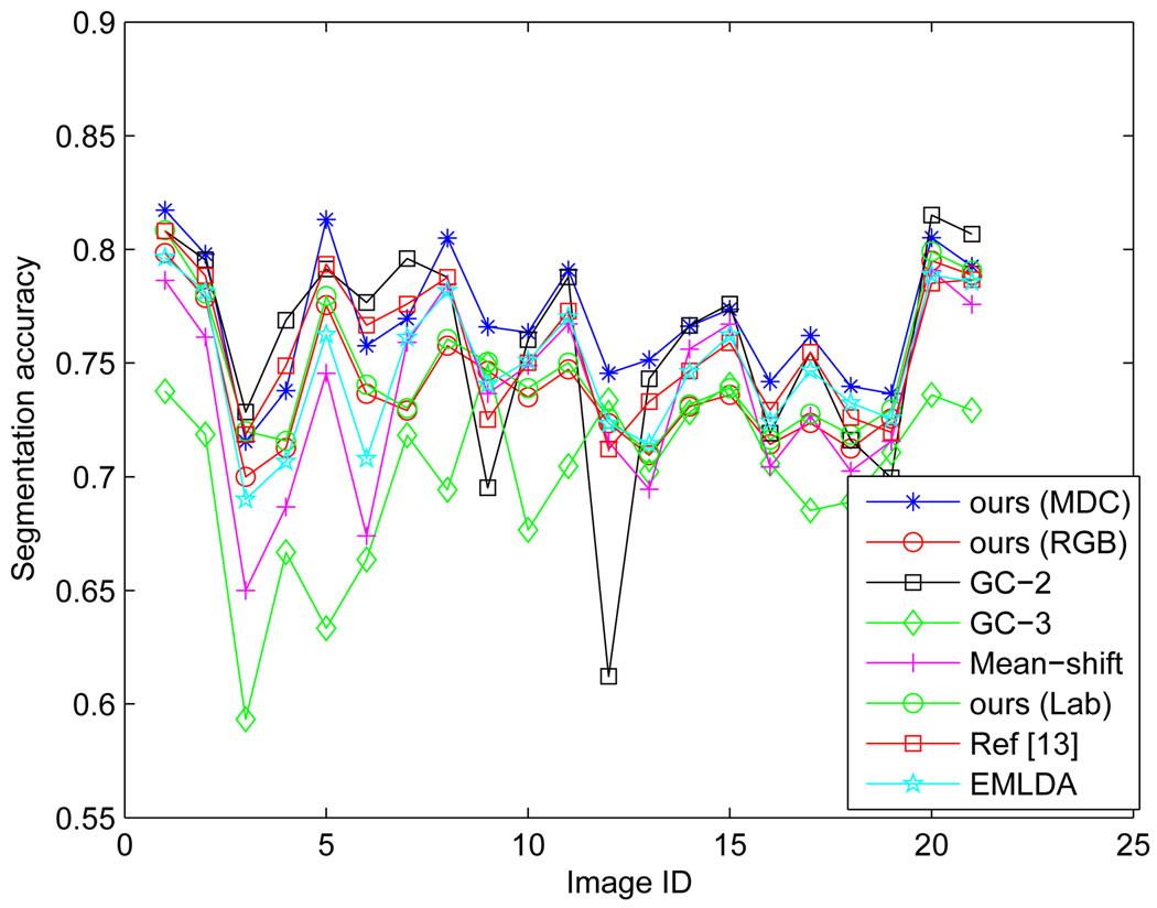
For each compared algorithm, we get a black and white (binary) image whose white pixels correspond to the cell-nuclei regions. Let A be the binary image produced by our method and B be the ground-truth mask, the cell-nuclei segmentation accuracy can be computed as $\text{Acc}=\frac{A\cap B}{A\cup B}$. In this way, the segmentation accuracy is computed for GC-2, GC-3 and Mean-shift, EMLDA, and Al-Kofahi et al’s [13] algorithms, respectively. The comparison of segmentation performance is shown in Fig.15. Table III shows the mean and variance of the segmentation accuracy achieved by the compared algorithms.

Fig. 15.

Comparison of segmentation performance with Graph-cut [10], Mean-shift [11], EMLDA [12] and Al-Kofahi et al.’s method [13]

TABLE III.

Comparison of segmentation performance with respect to the average and variance of the segmentation accuracy as shown in Fig.15

	ours (MDC)	ours (RGB)	ours (Lab)	GC-2
mean	0.769	0.7417	0.7429	0.7573
variance	8.1661e-004	8.8010e-004	8.6904e-004	0.0024
	Mean-shift	[13]	EMLDA	GC-3
mean	0.7357	0.7515	0.7426	0.7008
variance	0.0016	0.0011	0.0013	0.0015

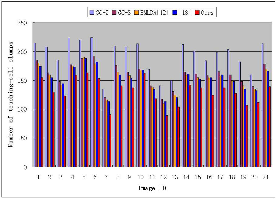
For the Graph-cut algorithm, the segmentation results will be different if the initialized number of object classes is different. For example, the image can be partitioned into cell-nuclei and extra-nuclei regions if the number of object classes is set to two, and into cell-nuclei, extra-cellular, and background regions if the number of object classes is set to three. Correspondingly, we have set two and three object classes for the Graph-cut algorithm, respectively, which is denoted as GC-2 and GC-3 in short. By checking Table III, we observe that GC-2 cannot consistently achieve good performance across the 21 test images as the method proposed in this paper, and GC-3 is even worse than GC-2. In addition, we also find that the segmentation results obtained by GC-2 has an important disadvantage when compared to our method for the next-step touching-cell splitting, since GC-2 tends to produce more touching-cell clumps than our algorithms. Fig.14 shows the comparison of the proposed segmentation algorithm with GC-2 and GC-3 in producing the number of touching-cell clumps before the splitting step.

Fig. 14.

Comparison of segmentation performance with GC-2/GC-3, EMLDA [12] and Al-Kofahi et al.’s method [13] in terms of the number of produced touching-cell clumps before the splitting step

For Mean-shift algorithm, we use the EDISON software which is free for downloading [48]. The most accurate segmentation performance by EDISON is obtained when the two parameters, h_s and h_r, are tuned to 9 and 8, respectively. We find that Mean-shift can generally achieve better performance than GC-3, and performs worse than GC-2 for most test images. To demonstrate that the generated MDC color space is more discriminant than the RGB space in classification performance based on the extracted LFT features, we directly apply the proposed segmentation method on the RGB space. This can be done by extracting the LFT feature in the RGB space and make a classification of each pixel afterwards. Our algorithm on MDC color space can achieve about an average of 2.8% improvement in segmentation accuracy on the 21 test images. In addition, we have also tested our segmentation algorithm in the Lab color space, and our algorithm can achieve about 2.5% improvement. The comparisons are shown in Fig.15 and Table III.

The Superpixel algorithm partitions the image into many small disjoint areas by boundary pixels, however, it does not explicitly specify which class each individual small area belongs to. Therefore, we compare the segmentation accuracy of the Superpixel algorithm with our segmentation algorithm in a different way. We look for errors that occur where the Superpixel algorithm does not correctly place the boundary on a cell nuclei. Table IV shows the comparison between our algorithm and the Superpixel method (note that the original Superpixel source code is available online [49]). Since we know that there are averagely 5500 cells in each test image, we set the two parameters in the Superpixel source code (initial and final number of partitions) to 100 and 560, respectively, after tuning.

TABLE IV.

Comparison of segmentation performance with Superpixel algorithm.

Image ID	Error by Superpixel	Error by our algorithm
1	173	36
2	189	25
3	165	40
4	266	39
5	154	39
6	212	34
7	172	26
8	179	26
9	165	24
10	233	43
11	202	30
12	144	23
13	167	22
14	197	25
15	193	21
16	149	28
17	234	25
18	204	37
19	231	23
20	179	29
21	185	33
mean	190	30

The EMLDA algorithm can achieve approximately equivalent performance compared to Al-Kofahi et al’s segmentation method in terms of the numbers of produced touching-cell clumps by them, but about 1% worse than Al-Kofahi et al’s method in terms of segmentation accuracy. Both of them are worse than our segmentation algorithm in terms of the number of produced touching-cell clumps (25.4 more clumps than ours per image) and segmentation accuracy (at least 1% worse per image).

It should be noted that the contribution of our segmentation algorithm cannot be just evaluated by the improvement in average segmentation accuracy. This is due to the following fact: our algorithm is more successful in segmenting some important minor regions, e.g., the joining area of two touching cells. The segmentation of these minor areas are extremely important for the subsequent cell-splitting step since our ultimate goal is to partition the whole pathological image into single cells. However, since these minor regions only cover a very small portion of the whole image, the advantage of our segmentation over the others cannot be fully reflected by the marginal improvement if only based on the segmentation accuracy. Therefore, the number of produced touching-cell clumps is a more important measure for evaluating our segmentation method. In addition, another way to evaluate our algorithm is to compare the combination of our segmentation method + our splitting algorithm with the combinations of the other segmentation methods + our splitting algorithm. This comparison is to show the ultimate splitting accuracy, as shown in Table V and Table VI.

TABLE V.

Evaluation of splitting performance based on our segmentation method + our touching-cell splitting algorithm and the method proposed in [13]

Image ID	Number of cells	Correct split	Under- split	Over- split	Encroach. errors
1	593	557/525	19/33	8/15	9/20
2	495	460/444	12/20	7/17	6/14
3	362	322/297	4/14	28/36	8/15
4	719	680/653	25/36	8/18	6/12
5	565	526/502	8/16	23/32	8/15
6	733	699/673	21/30	7/17	6/13
7	464	438/417	12/19	9/15	5/13
8	533	507/485	6/13	11/16	9/19
9	507	483/460	6/14	7/15	11/18
10	718	675/656	20/29	13/19	10/14
11	558	528/507	10/17	9/18	11/16
12	422	399/378	9/17	6/11	8/16
13	518	496/477	9/16	9/15	4/10
14	632	607/581	12/22	7/16	6/13
15	585	564/540	9/21	6/12	6/12
16	537	509/485	10/19	13/20	5/13
17	611	586/568	13/20	5/11	7/12
18	614	577/558	18/25	8/15	11/16
19	605	582/560	11/19	7/14	5/12
20	565	536/517	12/22	9/15	8/11
21	624	591/574	13/19	11/18	9/13
Ave.	569.5	539.6/517	12.3/21	10.1/17.4	7.5/14.2

TABLE VI.

Results after applying other segmentation methods (Graph-Cut (GC-2/GC-3) and EMLDA, respectively) and our touching-cell splitting algorithm

Image ID	Num. of cells	Correct split	Under- split	Over- split	Encroach. errors
1	593	520/539/537	32/23/20	19/15/22	22/16/14
2	495	415/453/444	31/17/15	20/15/24	29/10/12
3	362	266/305/297	20/7/7	49/37/44	27/13/14
4	719	633/666/660	55/32/35	16/11/15	15/10/9
5	565	481/515/496	14/10/13	54/29/44	16/11/12
6	733	652/673/668	48/33/35	16/13/18	17/14/12
7	464	405/419/406	23/18/22	19/14/20	17/13/16
8	533	468/484/479	20/13/16	27/22/26	18/14/12
9	507	443/460/461	18/14/14	24/17/14	22/16/18
10	718	649/668/664	28/24/21	20/14/19	21/12/14
11	558	492/514/510	19/16/17	22/14/20	25/14/11
12	422	368/383/375	16/14/14	18/13/18	20/12/15
13	518	468/475/475	18/15/13	16/19/20	16/9/10
14	632	552/586/583	30/17/19	28/12/15	22/17/15
15	585	508/540/535	28/16/19	25/14/19	24/15/12
16	537	470/483/485	24/20/17	29/21/22	14/13/13
17	611	547/561/565	32/22/20	14/12/14	18/16/12
18	614	540/548/555	30/26/24	20/19/17	24/21/18
19	605	529/548/546	35/24/27	22/16/18	19/17/14
20	565	507/517/522	23/18/16	18/16/15	17/14/12
21	624	564/565/564	31/22/20	23/17/21	24/20/19
Ave.	569.5	498/519/516	27/19/19	24/17/21	20/14/13

Through the experimental results, our algorithm has two advantages over the other compared ones: The first one, it can produce more accurate and robust nuclei segmentation (reflected by the consistently good performance in Fig. 15 and Table III). More importantly, the second advantage is that it can produce much fewer touching-cell clumps than the compared algorithms, as shown in Fig. 14. Additionally, the resulting touching-cell clumps by our segmentation algorithm are usually much smaller than the ones produced by the other methods, which makes it much easier for the subsequent splitting algorithm to successfully split these touching-cell clumps into single cells. This has been reflected (validated) by comparison results in Table V and Table VI.

C. Evaluation of splitting accuracy

To evaluate the splitting accuracy, we use the following types of errors: the under-splitting error, over-splitting error, and encroachment error. The under-splitting error occurs when the algorithm does not place a boundary between a pair of touching nuclei. The over-splitting error occurs when the algorithm places a boundary within a single non-touching cell. The encroachment error occurs when the splitting algorithm does not correctly place the boundary between a pair of touching nuclei. In other words, it is the error in delineating the true border between two nuclei. The under-splitting errors occur both in the group of separated non-touching cells and the group of touching-cell clumps. The over-splitting and encroachment errors occur mostly during the splitting of the touching-cell clumps.

We initially evaluate the accuracy in separating the touching-/non-touching cells. First, we calculate the number of false positives in the group of obtained non-touching cells per image (i.e., it should be a touching-cell clump, but classified as a non-touching cell). The number of these false positives in non-touching cells per image is listed as follows (the denominator is the total number of separated non-touching cells per image): 16/437, 2/364, 2/238, 13/558, 4/399, 7/579, 6/375, 3/393, 4/371, 12/555, 7/442, 4/335, 6/413, 6/491, 5/449, 6/412, 8/475, 10/485, 4/497, 7/451, 6/484. On the other hand, we also count the number of false positives in the group of obtained touching-cell clumps per image (i.e., it should be a non-touching cell, but classified as a touching-cell clump). These numbers are listed as follows(the denominator is the total number of separated touching-cell clumps per image): 5/156, 7/131, 9/124, 8/161, 8/166, 5/154, 8/89, 10/140, 7/136, 12/163, 9/116, 6/87, 8/105, 6/141, 6/136, 12/125, 5/136, 7/129, 7/108, 9/114, 11/114.

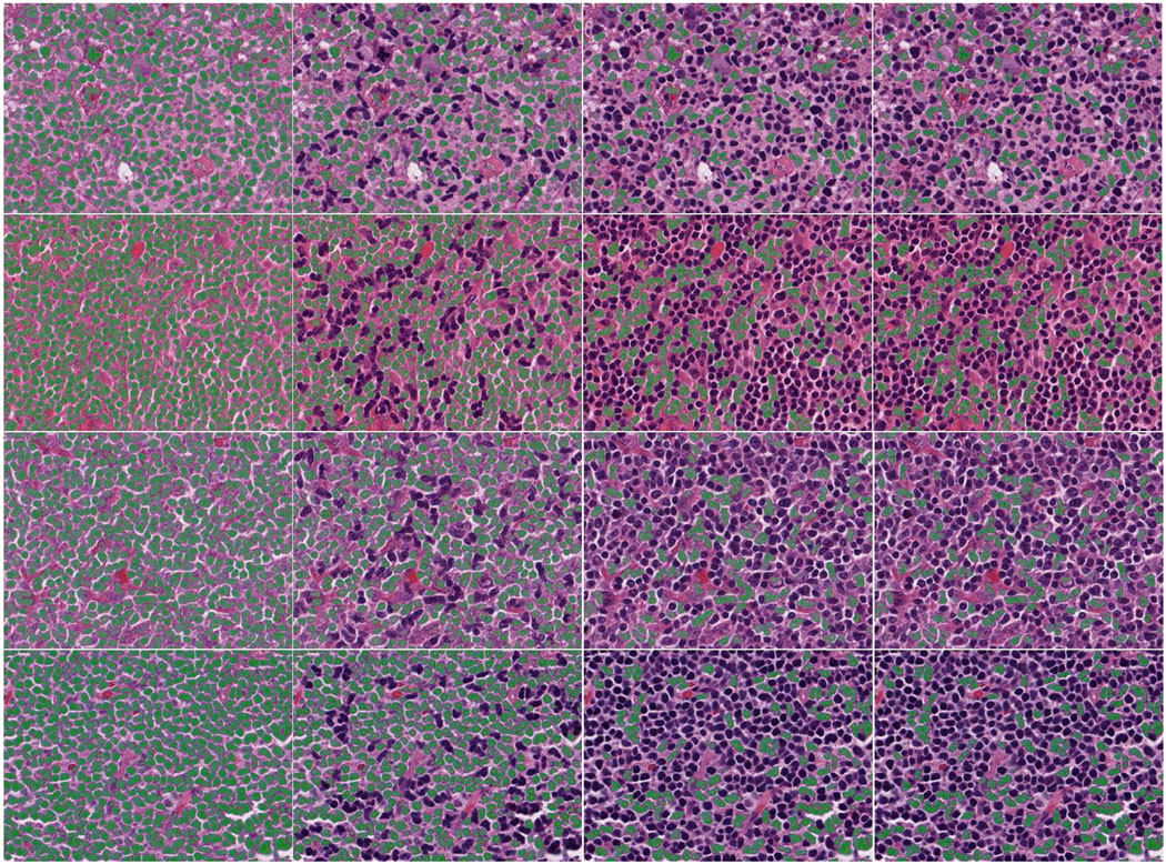
The total splitting accuracy is shown in Table V. Note that since the under-splitting errors occur both in the non-touching/touching-cell discrimination process and touching-cell splitting stage, the statistics of under-splitting error listed in Table V include errors in both cases. As a comparison, the h-minima marker-controlled watershed algorithm and the splitting algorithm proposed in [13] has been applied to our test images. In average, the watershed algorithm (h set to 2) has more than 144 under-splitting errors than our splitting algorithm. The over-splitting error (during splitting all the connected components in the segmentation map) is quite low, about 1.35% of the total number of split cells are over-split cells. In addition, we have also compared our splitting performance with [13] and the comparison is shown in Table V. Note that the source code (software) for [13] is available at [50]. This software automatically sets the optimal values for necessary parameters. On average, Al-Kofahi et al’s method [13] produces 22.6 more errors than our splitting algorithm. To check whether the splitting results by our method are significantly better than [13], we made a significance t-test with the following steps: we got the splitting error based on our method and the error based on [13] for each of the 21 test images. Then we computed the t value based on the two groups of errors. We got the value of 9.466 for t, which shows that our results are significantly better than [13] (t should approximately be at least 2.0 to reach significance level by looking up the t-distribution table). Since [13] can achieve better splitting result than the other compared methods, we just neglected the significance t-test for the other methods. Finally, four examples are given in Fig.16 to demonstrate the results of segmentation, non-touching/touching-cell discrimination, and touching-cell clump splitting (each row corresponding to one example).

Fig. 16.

Four examples of segmentation, non-touching/touching-cell discrimination, and touching-cell clump splitting (each row corresponding to one example). First column: segmentation results. Second column: non-touching cells. Third column: touching-cell clumps. Fourth column: split touching-cells

D. Evaluation of time-cost in segmentation

Our algorithm was originally implemented using Matlab (version 7.10.0). We tested our segmentation algorithm on 21 800×600 images. Originally, we run our Matlab code on a 64-bit Windows PC, which has a 2.4GHz CPU and a 4GB RAM. The average time-cost is about 7.3 minutes per image. It is important to note that we do not use any mex files. In comparison, the Graph-cut algorithm takes about 20 seconds with compiled mex files. The Mean-shift algorithm runs in 14 seconds with the freely downloaded EDISON software. The EMLDA (Matlab code) needs 6.6 minutes and Al-Kofahi et al’s software (written by Python) uses 22 seconds. The Superpixel is the most time-consuming one, which takes about 24 minutes per image, even using some compiled mex files. For a fair comparison, we have implemented our segmentation algorithm in C++. The time cost by our C++ implementation is about 28 seconds per image.

VI. CONCLUSION AND FUTURE WORK

In this paper, we propose an integrated framework consisting of a novel supervised cell-image segmentation algorithm and a new touching-cell splitting method. The segmentation algorithm learns a most discriminant color space in a linear discriminant framework so that the extracted local Fourier transform features can achieve optimal classification (segmentation) in it. We also propose an efficient LFT feature extraction scheme to speed up the segmentation process. In the touching-cell clump splitting step, we propose an novel strategy in that the touching-cell clump is differentiated from the non-touching cells beforehand, and only the touching-cell clump is split by a new iterative splitting algorithm.

The whole framework can produce accurate cell-nuclei segmentation and touching-cell splitting results, which are highly desirable for quite a number of applications, such as the automatic histopathological grading systems which carry out feature quantification on single cells before categorizing them by classification algorithms (note that, since the cell nuclei in cut-tissue images have elliptical boundaries in most cases, features based on cell shape can be readily quantified by applying a simple ellipse-fitting algorithm to the single spit cells obtained by our method). In our future work, we will use the output of the proposed framework for grading of Lymphoma diseases based on detection a typical type of cancer cells (e.g., Centroblast).

APPENDIX

A. Complexity analysis of the brute-force and fast LFT feature extraction methods

The complexity in extracting an LFT feature from each pixel during segmentation can be analyzed as follows: the complexity of the brute-force method is 𝒪(n_k × n_m × p² × D²) + 𝒪(n_mc × 𝒪(mean) × D²), where the first item refers to the complexity of producing L_i, i = 1, 2, …, 8, while the second item refers to the complexity of computing eight means at each pixel location. The n_k refers to the number of kernels (n_k=8), the n_m to the number of multiplication operation in convolving with each kernel (n_m=8), the n_mc to the number of mean computation (n_mc=8). The p is the size of the local neighborhood at each pixel 𝒪(mean) is the complexity of computing a mean of each pixel’s local neighborhood, which involves p² addition and one multiplication operations. For efficiency, the mean operation is replaced by sum operation in practice, which can speed up the feature extraction process without sacrificing segmentation performance. 𝒪(mean) can thus be represented by p² addition operations. We use D² to represent the number of pixels in the whole image. Therefore, the complexity of extraction LFT feature at every pixel of the whole image in a brute-force way consists of 8 × 8 × p² × D² multiplication and 8 × p² × D² addition operations, i.e., 7744 × D² multiplication and 968 × D² addition operations when p is set to 11 in our paper.

In comparison, the complexity of segmentation based on the proposed efficient LFT feature extraction can be estimated as follows: $8\times 𝒪(\mathit{\text{shifting}})+{\displaystyle {\sum }_{i=1}^8𝒪(L_i)+}{\displaystyle {\sum }_{i=1}^8𝒪(i{L}_i)+}𝒪(8\times 𝒪(\mathit{\text{mean}})\times D^2)$, where 𝒪(shifting) is the complexity of shifting an image, ${\displaystyle {\sum }_{i=1}^8𝒪(L_i)}$ corresponding to the complexity of calculating L_i, i = 1, 2, …, 8, ${\displaystyle {\sum }_{i=1}^8𝒪(i{L}_i)}$ corresponding to the complexity of building integral maps iL_i, i = 1, 2, …, 8 from L_i and 𝒪(8 × 𝒪(mean) × D²) to the complexity of computing means at each pixel of iL_i. It should be noted that 𝒪(mean) here only involves four addition and one multiplication operations. Likewise, this mean operation is also replaced by sum operation for efficiency. 𝒪(mean) can thus be represented by four addition operations here. Therefore, 𝒪(8 × 𝒪(mean) × D²) equals to 8 × 4 × D² addition operations. ${\displaystyle {\sum }_{i=1}^8𝒪(i{L}_i)}$ is also equivalent to 8 × 4 × D² addition operations. ${\displaystyle {\sum }_{i=1}^8𝒪(L_i)}$ has 40 × D² addition and 4 × D² multiplication operations. Therefore, the total complexity can be approximated as 104 × D² addition and 4 × D² multiplication operations by ignoring the time used for shifting an image.

By assuming that the complexity of multiplication is t times that of addition, theoretically, we can approximately achieve $\frac{7744t+968}{4t+104}$ (e.g., 147 if let t be 2 with new processor architecture) times faster than brute-force one. However, in practice, we can achieve about 120±6.8 times speed improvement (in an experiment involving 10 tries). The reasons can be: (1) the shifting of images takes small but finite amount of time; (2) it takes longer for the efficient feature extraction algorithm to access memory.

B. Proofs of Lemma 1 and Lemma 2

Lemma 1: The row vectors of Φ_sw (or Φ̃_sw) are linearly independent.

Proof: First, we prove that the row vectors of Φ_sw are linearly independent. For convenience, we denote the j-th training image patch of class i as T_ij.

Since Φ_sw = [(Q₁₁ − M₁), …, (Q_cNc − M_c)], where Q_ij ∈ ℝ^8×3, i = 1, 2, j = 1, …, N_i is an LFT feature matrix extracted from T_ij. Reminiscent of the fact that the k-th row of Q_ij is the first-order moment feature of L_k, and L_k is the result of applying kernel F_k to T_ij (in RGB channels, denoted by ${\mathbf{T}}_{\mathit{\text{ij}}}^r,{\mathbf{T}}_{\mathit{\text{ij}}}^g\text{ and }{\mathbf{T}}_{\mathit{\text{ij}}}^b$, respectively).

Let f_k ∈ ℝ^9×1 be the kernel vector formed by concatenating each column of F_k. Let ${\mathbf{l}}_{u,\upsilon }^r\in {ℝ}^{9\times 1}$ be the column vector formed by concatenating each column of the 3×3 local neighborhood of pixel (u,v) of ${\mathbf{T}}_{\mathit{\text{ij}}}^r$. Correspondingly, ${\mathbf{l}}_{u,\upsilon }^g\in {ℝ}^{9\times 1}\text{ and }{\mathbf{l}}_{u,\upsilon }^b\in {ℝ}^{9\times 1}$ refer to G and B channels, respectively.

Mathematically, the k-th row of Q_ij is

$$\begin{array}{cc}\left[{\mathbf{Q}}_{\mathit{\text{ij}}}^{k1},{\mathbf{Q}}_{\mathit{\text{ij}}}^{k2},{\mathbf{Q}}_{\mathit{\text{ij}}}^{k3}\right]\hfill & =\frac{1}{\tau }{\displaystyle \sum _{u=2}^{h-1}}{\displaystyle \sum _{\upsilon =2}^{w-1}}\left[{\mathbf{f}}_k^T{\mathbf{l}}_{u,\upsilon }^r,{\mathbf{f}}_k^T{\mathbf{l}}_{u,\upsilon }^g,{\mathbf{f}}_k^T{\mathbf{l}}_{u,\upsilon }^b\right]\hfill \\ \hfill & ={\mathbf{f}}_k^T{\mathrm{\Gamma }}_{\mathit{\text{ij}}}\hfill \end{array}$$ (25)

where h and w correspond to the height and width of T_ij, $\tau =(h-2)\times (w-2),{\mathrm{\Gamma }}_{\mathit{\text{ij}}}=\frac{1}{\tau }{\displaystyle {\sum }_{u=2}^{h-1}{\displaystyle {\sum }_{\upsilon =2}^{w-1}\left[{\mathbf{l}}_{u,\upsilon }^r,{\mathbf{l}}_{u,\upsilon }^g,{\mathbf{l}}_{u,\upsilon }^b\right]}}$, and Γ_ij ∈ ℝ^9×3.

Accordingly, Q_ij can be represented as

$${\mathbf{Q}}_{\mathit{\text{ij}}}={[{\mathrm{\Gamma }}_{\mathit{\text{ij}}}^T{\mathbf{f}}_1,{\mathrm{\Gamma }}_{\mathit{\text{ij}}}^T{\mathbf{f}}_2,\dots ,{\mathrm{\Gamma }}_{\mathit{\text{ij}}}^T{\mathbf{f}}_8]}^T$$ (26)

and M_i is represented as

$$\begin{array}{cc}{\mathbf{M}}_i\hfill & =\frac{1}{N_i}{\displaystyle \sum _{j=1}^{N_i}}{\mathbf{Q}}_{\mathit{\text{ij}}}\hfill \\ \hfill & ={[\frac{1}{N_i}{\displaystyle \sum _{j=1}^{N_i}}{\mathrm{\Gamma }}_{\mathit{\text{ij}}}^T{\mathbf{f}}_1,\frac{1}{N_i}{\displaystyle \sum _{j=1}^{N_i}}{\mathrm{\Gamma }}_{\mathit{\text{ij}}}^T{\mathbf{f}}_2,\dots ,\frac{1}{N_i}{\displaystyle \sum _{j=1}^{N_i}}{\mathrm{\Gamma }}_{\mathit{\text{ij}}}^T{\mathbf{f}}_8]}^T\hfill \\ \hfill & ={[{\mathbf{Z}}_i^T{\mathbf{f}}_1,{\mathbf{Z}}_i^T{\mathbf{f}}_2,\dots ,{\mathbf{Z}}_i^T{\mathbf{f}}_8]}^T\hfill \end{array}$$ (27)

Therefore, Φ_sw can be explicitly represented as

$${\mathbf{\Phi }}_{\mathit{\text{sw}}}=\left(\begin{array}{cccc}{\mathbf{f}}_1^T({\mathrm{\Gamma }}_{11}-{\mathbf{Z}}_1)& {\mathbf{f}}_1^T({\mathrm{\Gamma }}_{12}-{\mathbf{Z}}_1)& \cdots & {\mathbf{f}}_1^T({\mathrm{\Gamma }}_{{\mathit{\text{cN}}}_c}-{\mathbf{Z}}_c)\\ {\mathbf{f}}_2^T({\mathrm{\Gamma }}_{11}-{\mathbf{Z}}_1)& {\mathbf{f}}_2^T({\mathrm{\Gamma }}_{12}-{\mathbf{Z}}_1)& \cdots & {\mathbf{f}}_2^T({\mathrm{\Gamma }}_{{\mathit{\text{cN}}}_c}-{\mathbf{Z}}_c)\\ ⋮& ⋮& \ddots & ⋮\\ {\mathbf{f}}_8^T({\mathrm{\Gamma }}_{11}-{\mathbf{Z}}_1)& {\mathbf{f}}_8^T({\mathrm{\Gamma }}_{12}-{\mathbf{Z}}_1)& \cdots & {\mathbf{f}}_8^T({\mathrm{\Gamma }}_{{\mathit{\text{cN}}}_c}-{\mathbf{Z}}_c)\end{array}\right)$$

Or we can reformulate Φ_sw more concisely,

$${\mathbf{\Phi }}_{\mathit{\text{sw}}}=\left(\begin{array}{c}{\mathbf{f}}_1^T\mathbf{V}\\ {\mathbf{f}}_2^T\mathbf{V}\\ ⋮\\ {\mathbf{f}}_8^T\mathbf{V}\end{array}\right)$$

Let K = [k₁, k₂, …, k8]^T, let

$$k_1{\mathbf{f}}_1^T\mathbf{V}+k_2{\mathbf{f}}_1^T\mathbf{V}+,\dots ,+k_8{\mathbf{f}}_8^T\mathbf{V}=\mathbf{0}$$ (28)

We notice that the dimension of V is $9\times 3\times {\displaystyle {\sum }_{i=1}^c{N}_i}$ (9 × 4500 in this paper), whose row vectors are linearly independent because of the variety of texture in training samples (not all of the training samples have uniform patterns, e.g., purely black or white). We have also observed through extensive experiments that this assumption is valid. Therefore, VV^T is invertible. We have,

$$k_1{\mathbf{f}}_1^T{\mathbf{\text{VV}}}^T{({\mathbf{\text{VV}}}^T)}^{-1}+,\dots ,+k_8{\mathbf{f}}_8^T{\mathbf{\text{VV}}}^T{({\mathbf{\text{VV}}}^T)}^{-1}=\mathbf{0}$$ (29)

That is,

$$k_1{\mathbf{f}}_1^T+k_2{\mathbf{f}}_1^T+,\dots ,+k_8{\mathbf{f}}_8^T=\mathbf{0}$$ (30)

We can conclude that k₁ = k₂ =,…, = k₈ = 0 based on the fact that ${\mathbf{f}}_i^T{\mathbf{f}}_j=0$ for any i,j, and i ≠ j. Therefore, the row vectors of Φ_sw are linearly independent. A similar proof can be derived for Φ̃_sw.

Lemma 2: The $({\mathbf{\Phi }}_{\mathit{\text{sb}}}{\mathbf{\Delta }}_{\mathit{\text{sb}}}{\mathbf{\Delta }}_{\mathit{\text{sb}}}^T{\mathbf{\Phi }}_{\mathit{\text{sb}}}^T)\mathbf{P}=({\mathbf{\Phi }}_{\mathit{\text{sw}}}{\mathbf{\Delta }}_{\mathit{\text{sw}}}{\mathbf{\Delta }}_{\mathit{\text{sw}}}^T{\mathbf{\Phi }}_{\mathit{\text{sw}}}^T)\mathbf{P}\mathrm{\Lambda }$ is a well-posed generalized eigenvalue problem (S₃ of Table I).

Proof: We have known that ${\mathbf{\Phi }}_{\mathit{\text{sw}}}{\mathbf{\Delta }}_{\mathit{\text{sw}}}{\mathbf{\Delta }}_{\mathit{\text{sw}}}^T{\mathbf{\Phi }}_{\mathit{\text{sw}}}^T={\tilde{\mathbf{\Phi }}}_{\mathit{\text{sw}}}{\tilde{\mathbf{\Phi }}}_{\mathit{\text{sw}}}^T$, and the dimension of Φ̃_sw is $8\times 3{\displaystyle {\sum }_{i=1}^c{N}_i}$ (note that N_i is the number of training image patches of class i). It is also known that $\text{rank}({\tilde{\mathbf{\Phi }}}_{\mathit{\text{sw}}}{\tilde{\mathbf{\Phi }}}_{\mathit{\text{sw}}}^T)=\text{rank}({\tilde{\mathbf{\Phi }}}_{\mathit{\text{sw}}}^T{\tilde{\mathbf{\Phi }}}_{\mathit{\text{sw}}})=\text{rank}({\tilde{\mathbf{\Phi }}}_{\mathit{\text{sw}}})=\text{rank}({\tilde{\mathbf{\Phi }}}_{\mathit{\text{sw}}}^T)$. Based on Lemma 1, rank(Φ̃_sw)=8. Since the dimension of ${\mathbf{\Phi }}_{\mathit{\text{sw}}}{\mathbf{\Delta }}_{\mathit{\text{sw}}}{\mathbf{\Delta }}_{\mathit{\text{sw}}}^T{\mathbf{\Phi }}_{\mathit{\text{sw}}}^T$ is 8×8, we can show that ${\mathbf{\Phi }}_{\mathit{\text{sw}}}{\mathbf{\Delta }}_{\mathit{\text{sw}}}{\mathbf{\Delta }}_{\mathit{\text{sw}}}^T{\mathbf{\Phi }}_{\mathit{\text{sw}}}^T$ is full rank. Therefore, it is equivalent to solving ${\left({\mathbf{\Phi }}_{\mathit{\text{sw}}}{\mathbf{\Delta }}_{\mathit{\text{sw}}}{\mathbf{\Delta }}_{\mathit{\text{sw}}}^T{\mathbf{\Phi }}_{\mathit{\text{sw}}}^T\right)}^{-1}\left({\mathbf{\Phi }}_{\mathit{\text{sb}}}{\mathbf{\Delta }}_{\mathit{\text{sb}}}{\mathbf{\Delta }}_{\mathit{\text{sb}}}^T{\mathbf{\Phi }}_{\mathit{\text{sb}}}^T\right)\mathbf{P}=\mathbf{P}\mathrm{\Lambda }$.

REFERENCES

- 1.Gurcan M, Boucheron L, Can A, Madabhushi A, Rajpoot N, Yener B. Histopathological image analysis: A review. IEEE Reviews in Biomedical Engineering. 2009;vol. 2:147–171. doi: 10.1109/RBME.2009.2034865. [DOI] [PMC free article] [PubMed] [Google Scholar]
- 2.Jeffe E, Harris N, Stein H, Vardiman J. Tumours of haematopoietic and lymphoid tissues. Lyon: IRAC Press; 2001. [Google Scholar]
- 3.Metter GE, Nathwani BN, Burke JS, Winberg CC, Mann RB, B M, et al. Morphological subclassification of follicular lymphoma: Variability of diagnoses among hematopathologists, a collaborative study between the repository center and pathology panel for lymphoma clinical studies. Journal of Clinical Oncology. 1985;vol. 3:25–38. doi: 10.1200/JCO.1985.3.1.25. [DOI] [PubMed] [Google Scholar]
- 4.Dick F, Lier SV, Banks P, Frizzera G, Witrak G, G R, et al. Use of the working formulation for non-hodgkin’s lymphoma in epidemiological studies: Agreement between reported diagnoses and a panel of experienced pathologists. Journal of National Cancer Institue. 1987;vol. 78:1137–1144. [PubMed] [Google Scholar]
- 5.T. N.-H. L. C. Project. A clinical evaluation of the international lymphoma study group classification of non-hodgkin lymphoma. Blood. 1997;vol. 89:3909–3918. [PubMed] [Google Scholar]
- 6.Zhou F, Feng J-F, yun Shi Q. Texture feature based on local fourier transform; Proceedings of IEEE International Conference on Image Processing; 2001. pp. 610–613. [Google Scholar]
- 7.Yu H, Li M, Zhang H-J, Feng J. Color texture moments for content-based image retrieval. Proceedings of IEEE International Conference on Image Processing. 2002;vol. 3:929–933. [Google Scholar]
- 8.Viola P, Jones MJ. Robust real-time face detection. International Journal of Computer Vision. 2004;vol. 57(no. 2):137–154. [Google Scholar]
- 9.Ren X, Malik J. Learning a classification model for segmentation. Proceedings of International Conference on Computer Vision. 2003;vol. 1:10–17. [Google Scholar]
- 10.Boykov Y, Jolly M-P. Interactive graph cuts for optimal boundary and region segmentation of objects in nd images. Proceedings of IEEE International Conference on Computer Vision. 2001;vol. 1:105–112. [Google Scholar]
- 11.Comaniciu D, Meer P. Mean shift: A robust approach toward feature space analysis. IEEE Transactions on Pattern Analysis and Machine Intelligence. 2002;vol. 24(no. 5):603–619. [Google Scholar]
- 12.Kong J, Sertel O, Shimada H, Boyer K, Saltz J, Gurcan M. Computer-aided evaluation of neuroblastoma on whole-slide histology images: Classifying grade of neuroblastic differentiation. Pattern Recognition. 2009;vol. 42(no. 6):1080–1092. doi: 10.1016/j.patcog.2008.10.035. [DOI] [PMC free article] [PubMed] [Google Scholar]
- 13.Al-Kofahi Y, Lassoued W, Lee W, Roysam B. Improved automatic detection and segmentation of cell nuclei in histopathology images. IEEE Transactions on Biomedical Engineering. 2009;vol. 57(no. 4):841–852. doi: 10.1109/TBME.2009.2035102. [DOI] [PubMed] [Google Scholar]
- 14.Duda RO, Hart PE, Stork DG. Pattern classification (2nd edition) John Wiley & Sons, Inc; 2001. [Google Scholar]
- 15.Shi J, Malik J. Normalized cuts and image segmentation. IEEE Transactions on Pattern Analysis and Machine Intelligence. 2000;vol. 22(no. 8):888–905. [Google Scholar]
- 16.Li SZ. Markov random field modeling in computer vision. Springer-Verlag; 2001. [Google Scholar]
- 17.Vese LA, Chan TF. A multiphase level set framework for image segmentation using the mumford and shah model. International Journal of Computer Vision. 2002;vol. 50(no. 3):271–293. [Google Scholar]
- 18.Haralick KSRM, Dinstein Textural features for image classification. IEEE Transactions on Systems, Man, and Cybernetics, Part C. 1973;vol. 3:610–621. [Google Scholar]
- 19.Qureshi H, Sertel O, Rajpoot N, Wilson R, Gurcan MN. Adaptive discriminant wavelet packet transform and local binary patterns for meningioma subtype classification. IEEE Conference on Medical Image Computing and Computer Assisted Intervention (MICCAI) 2008;vol. 2:196–204. doi: 10.1007/978-3-540-85990-1_24. [DOI] [PubMed] [Google Scholar]
- 20.Fernandez DC, Bhargava R, Hewitt SM, Levin IW. Infrared spectroscopic imaging for histopathologic recognition. Nature Biotechnology. 2005;vol. 23:469–474. doi: 10.1038/nbt1080. [DOI] [PubMed] [Google Scholar]
- 21.Sun N, Xu S, Cao M, Li J. Segmenting and counting of wall-pasted cells based on gabor filter; International Conference on Engineering in Medicine and Biology Society (EMBS); 2005. pp. 3324–3327. [DOI] [PubMed] [Google Scholar]
- 22.Wen Q, Chang H, Parvin B. A delunay triangulation approach for segmenting clumps of nuclei; IEEE International Symposium on Biomedical Imaging - from nano to macro; 2009. [Google Scholar]
- 23.Yang L, Meer P, Foran D. Unsupervised segmentation based on robust estimation and color active contour models. IEEE Transactions on Information Technology in Biomedicine. 2005;vol. 9(no. 3):475–486. doi: 10.1109/titb.2005.847515. [DOI] [PubMed] [Google Scholar]
- 24.Sertel O, Kong J, Catalyurek U, Lozanski G, Saltz J, Gurcan M. Histopathological image analysis using model-based intermediate representation and color texture: Follicular lymphoma grading. Journal of Signal Processing Systems. 2009;vol. 55(no. 1):169–183. [Google Scholar]
- 25.Zhou X, Liu K-Y, Bradley P, Perrimon N, Wong ST. Towards automated cellular image segmentation for rnai genome-wide screening. IEEE Conference on Medical Image Computing and Computer Assisted Intervention (MICCAI) 2005;vol. 1:885–892. doi: 10.1007/11566465_109. [DOI] [PubMed] [Google Scholar]
- 26.Sertel O, Lozanski G, Shana’ah A, Gurcan M. Computer-aided detection of centroblasts for follicular lymphoma grading using adaptive likelihood based cell segmentation. IEEE Transactions on Biomedical Engineering, to appear in the special issue on Multi-Parameter Optical Imaging and Image Analysis. 2011 doi: 10.1109/TBME.2010.2055058. [DOI] [PMC free article] [PubMed] [Google Scholar]
- 27.Vincent L, Soille P. Watersheds in digital spaces: an efficient algorithm based on immersion simulations. IEEE Transactions on Pattern Analysis and Machine Intelligence. 1991;vol. 13(no. 6):583–598. [Google Scholar]
- 28.Gran V, Mewes AUJ, Alcaniz M, Kikinis R, Warfield SK. Improved watershed transform for medical image segmentation using prior information. IEEE Transactions on Medical Imaging. 2004;vol. 23(no. 4):447–458. doi: 10.1109/TMI.2004.824224. [DOI] [PubMed] [Google Scholar]
- 29.Nedzved A, Pitas I. Morphological segmentation of histology cell images. IEEE International Conference on Pattern Recognition. 2000;vol. 1 [Google Scholar]
- 30.Fatakdawala H, Xu J, Basavanhally A, Bhanot G, Ganesan S, Feldman M, Tomaszewski J, Madabhushi A. Expectation maximization driven geodesic active contour with overlap resolution (emagacor): Application to lymphocyte segmentation on breast cancer histopathology. IEEE Transactions on Biomedical Engineering. 2010;vol. 57(no. 7):1676–1689. doi: 10.1109/TBME.2010.2041232. [DOI] [PubMed] [Google Scholar]
- 31.Sethian JA. Level set methods: Evolving interfaces in geometry, fluid mechanics, computer vision and materials sciences. 1st edition. Cambridge University Press; 1996. [Google Scholar]
- 32.Mukherjee DP, Ray N, Acton S. Level set analysis for leukocyte detection and tracking. IEEE Transactions on Image Processing. 2004;vol. 13(no. 4):562–572. doi: 10.1109/tip.2003.819858. [DOI] [PubMed] [Google Scholar]
- 33.Zhang Q, Pless R. Segmenting multiple familiar objects under mutual occlusion; IEEE Int. Conf. on Image Processing; 2006. [Google Scholar]
- 34.Paragios N, Rousson M. Shape priors for level set representation; European Conference on Computer Vision; 2002. pp. 78–92. [Google Scholar]
- 35.Bresson X, Vandergheynst P, Thiran J. A priori information in image segmentation: energy functional based on shape statistical model and image information; IEEE Int. Conf. on Image Processing; 2003. pp. 425–428. [Google Scholar]
- 36.Mao K, Zhao P, Tan P-H. Supervised learning-based cell image segmentation for p53 immunohistochemistry. IEEE Transactions on Biomedical Engineering. 2006;vol. 53(no. 6):1153–1163. doi: 10.1109/TBME.2006.873538. [DOI] [PubMed] [Google Scholar]
- 37.Naik S, Doyle S, Feldman M, Tomaszewski J, Madabhushi A. Gland segmentation and computerized gleason grading of prostate histology by integrating low-, high-level and domain specific information; The Second international workshop on Microscopic Image Analysis with Applications in Biology (MIAAB); 2007. [Google Scholar]
- 38.Naik S, Doyle S, Agner S, Madabhushi A, Tomaszeweski J, Feldman M. Automated gland and nuclei segmentation for grading of prostate and breast cancer histopatholog; IEEE International Symposium on Biomedical Imaging, Special Workshop on Computational Histopathology (CHIP); 2008. p. 284C287. [Google Scholar]
- 39.Otsu N. A threshold selection method from gray-level histograms. IEEE Transactions on System, Man, and Cybernatics. 1979;vol. 9(no. 1):62–66. [Google Scholar]
- 40.Loy G, Zelinsky A. Fast radial symmetry for detecting points of interest. IEEE Trans. on Pattern Analysis and Machine Intelligence. 2003;vol. 25(no. 8):959–973. [Google Scholar]
- 41.Soille P. Morphological image analysis: Principles and applications. Berlin, Germany: Springer-Verlag; 1999. [Google Scholar]
- 42.Cheng J, Rajapakse J. Segmentation of clustered nuclei with shape markers and marking function. IEEE Transactions on Biomedical Engineering. 2009;vol. 56(no. 3):741–748. doi: 10.1109/TBME.2008.2008635. [DOI] [PubMed] [Google Scholar]
- 43.Schmitt O, Hasse M. Radial symmetries based decomposition of cell clusters in binary and gray level images. Pattern Recognition. 2008;vol. 41(no. 6):1905–1923. [Google Scholar]
- 44.Keenan SJ, Diamond J, McCluggage WG, Bharucha H, Thompson D, Bartels PH, Hamilton PW. An automated machine vision system for the histological grading of cervical intraepithelial neoplasia (cin) Journal of Pathology. 2000;vol. 192(no. 3):351–362. doi: 10.1002/1096-9896(2000)9999:9999<::AID-PATH708>3.0.CO;2-I. [DOI] [PubMed] [Google Scholar]
- 45.Yang L, Tuzel O, Meer P, Foran DJ. Automatic image analysis of histopathology specimens using concave vertex graph. International Conference on Medical Image Computing and Computer Assisted Intervention (MACCAI) 2008;vol. 1:833–841. doi: 10.1007/978-3-540-85988-8_99. [DOI] [PMC free article] [PubMed] [Google Scholar]
- 46.Cong C, Parvin B. Model based segmentation of nuclei. IEEE International Confernce on Computer Vision and Pattern Recognition. 1999;vol. 1 [Google Scholar]
- 47.Zahn CT, Roskies RZ. Fourier descriptors for plane closed curves. IEEE Transactions on Computers. 1972;vol. C(no. 21):269–281. [Google Scholar]
- 48.Code for the edge detection and image segmentation system. 2010 http://coewww.rutgers.edu/riul/research/code/EDISON/index.html.
- 49.Superpixel source code. 2010 http://www.cs.sfu.ca/mori/research/superpixels/
- 50.source code for “improved automatic detection and segmentation of cell nuclei in histopathology images”. 2010 doi: 10.1109/TBME.2009.2035102. www.farsight-toolkit.org. [DOI] [PubMed]