

Abstract
This paper models the behavior of the longitudinal relaxation rate of the protons of tissue water R1 (R1 = 1/T1), measured in a Look-Locker (LL) experiment at 7 Tesla after administration of a paramagnetic contrast agent (CA). It solves the Bloch-McConnell equations for the longitudinal magnetization of the protons of water in a three-site two-exchange (3S2X) model with boundary conditions appropriate to repeated sampling of magnetization. The extent to which equilibrium intercompartmental water exchange kinetics affect monoexponential estimates of R1 after administration of a CA in dynamic contrast enhanced (DCE) experiment is described.
The relation between R1 and tissue CA concentration was calculated for CA restricted to the intravascular, or to the intravascular and extracellular compartments, by varying model parameters to mimic experimental data acquired in a rat model of cerebral tumor. The model described a nearly linear relationship between R1 and tissue concentration of CA, but demonstrated that the apparent longitudinal relaxivity of CA depends upon tissue type. The practical consequence of this finding is that the extended Patlak plot linearizes the ΔR1 data in tissue with leaky microvessels, accurately determines the influx rate of the CA across these microvessels, but underestimates the volume of intravascular blood water.
Keywords: Look Locker pulse sequence, relaxation rate constant, contrast mechanism, Bloch-McConnell’s equations, shutter-speed, water exchange rate
Introduction
Dynamic contrast enhanced MRI (DCE-MRI) often utilizes the assumption that a change in the tissue water protons’ longitudinal relaxation rate (ΔR1, where ΔR1 = Δ1/T1) induced by a paramagnetic MR contrast agent (CA) such as Gd-DTPA is proportional to the tissue concentration of CA and can therefore serve as a measure of CA tissue concentration as it varies with time. This concentration-time curve is then used to estimate vascular kinetic parameters in cerebral diseases such as stroke and tumors using a pharmacokinetic theory that is decades old (1–5). We, along with others, call this model “the standard model” (abbreviated as SM). The linear relationship between ΔR1 and tissue concentration has been thought to depend on the rapid exchange (relative to the ensemble’s longitudinal relaxation rate) of water protons between the different tissue compartments.
Contrariwise, it has been proposed that estimates of the relaxation rate of tissue water protons produced by using a single exponential as a model for the recovery of longitudinal magnetization may yield an estimate of tissue CA concentration that is significantly biased due to the finite rates of exchange of water protons between the tissue compartments (6,7). This latter work was conducted first in a 2-compartment model (2SX) that studied proton exchange across parenchymal cell membranes and essentially ignored the vascular contribution (7–11); later this was extended to a 3-compartment model (3SX) that included intravascular (blood), interstitial, and intracellular spaces (12–14). Because, in both the 2SX and 3SX models, the apparent longitudinal relaxivity of the tissue depends on the rate constants of intercompartmental water exchange, the model has been named by its authors the “shutter-speed model” (SSM). In a recent application, a 2-compartment (2SX) SSM that ignores the vascular compartment has shown promise in discriminating malignant lesions in breast cancer (13,14).
The SSM has recently been challenged (15). The basis of this challenge was twofold: 1) the SSM as implemented was held to be an incomplete representation of the actual experimental condition in typical DCE experiments, and 2) experimental fitting results for the standard model versus the SSM showed no advantage for the SSM. This latter result does not necessarily disprove the SSM; rather, it may point to the complexity of the SSM (5 free variables) in contrast to the standard model (1, 2, or 3 free variables) (5) and the consequent requirement of data with much higher signal-to-noise for the SSM.
The question as to how the change in an estimate of a single longitudinal rate constant relates to the tissue concentration of CA retains a great deal of practical significance in current clinical considerations. This paper proposes to particularize this question to Look-Locker (LL) studies in a rat model of cerebral tumor at 7 Tesla, and thus examine the operating characteristics of this approach to estimates of vascular permeability Ktrans. We emphasize that it is not the purpose of this paper to compare models – that is a much more complex task – but rather to examine in theory the response of tissue magnetization under a particular experimental condition. This paper addresses the theory of equilibrium intercompartmental water exchange in its complete form (12) with correct boundary conditions and both theory and modeling of a three-site two-exchange model (3S2X model) as applied to LL data at 7 Tesla, but does not account for blood inflow effects (16). The modeling results are used to examine the relation between a monoexponential estimate of tissue R1 and tissue CA concentration. The findings are that the apparent relaxivity of a CA in a given tissue does not vary appreciably over the course of a typical experiment. On the other hand, it is demonstrated that the apparent relaxivity of CA does vary between tissues, and thus lends a note of caution to a naïve interpretation of experimental results in a DCE estimate of vascular permeability.
Theory
Three-Site Two-Exchange Model
While there are many biological compartments in tissue, it is usually assumed that the protons associated with tissue water can be characterized as residing in one of three compartments: intravascular, extracellular, or intracellular with equilibrium water exchange kinetics taking place between these compartments (7,8,11,12). The water in red blood cells and in the plasma of the intravascular compartment is assumed to form a single compartment, since the protons of water exchange rapidly between the two moieties (mixing time ~10 ms (8), which is much shorter than the ensemble’s longitudinal relaxation time). On the other hand, water exchange between the intracellular and interstitial spaces (i.e., across parenchymal cellular membranes) and between the intravascular and the interstitial spaces (i.e., across the microvascular endothelium) are at least an order of magnitude slower than across the red blood cell membrane. It is generally assumed that there is little or no direct exchange of water between the intravascular space and the intracellular space via the intercellular tight junctions of the endothelium. For modeling longitudinal relaxation rate of tissue water protons, the intercompartmental equilibrium water exchange kinetics can thus be described by a linear three-site two-exchange [3S2X] model (12). A schematic diagram of a 3S2X model and its characteristic parameters is given in Figure 1.
Figure 1.
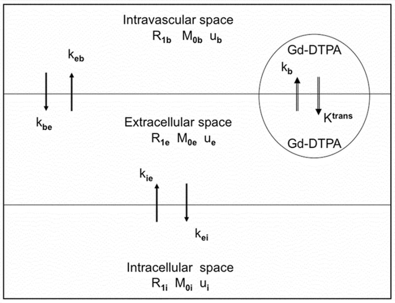
The three-site two-exchange (3S2X) model. R1b, R1e, and R1i are the longitudinal relaxation rates of the protons of water in the blood, interstitial, and intracellular spaces, respectively. Mob, Moe, and M0i are equilibrium magnetizations of the protons in these three spaces, respectively; their corresponding fractional water protons sizes are ub, ue, and ui. The rate of the water protons exchange from the blood to extracellular space is kbe and from the extracellular space back to blood is keb. The rate of water protons exchange from intra- to extracellular space is kie and from extra- to intracellular space is kei. In general, paramagnetically labeled contrast agents (e.g., Gd-DTPA) can exchange between plasma and the extracellular space across a leaky endothelium but will not enter the intracellular space (vi). The bidirectional exchange of Gd-DTPA between the intravascular space and extracellular is described by the transvascular transfer rate constants Ktrans and kb, respectively.
Under equilibrium exchange, the Bloch–McConnell equations describe the longitudinal magnetization of water protons in each pool of a 3S2X system (17):
| [1] |
where Mb, Me and Mi are the time-dependent longitudinal magnetizations of the water protons in the blood, interstitial, and parenchymal intracellular spaces, respectively. M0b, M0e, and M0i denote their equilibrium magnetization in the main magnetic field. R1b, R1e, and R1i are the longitudinal relaxation rate constants of the water protons in the absence of exchange within the blood, interstitium, and intracellular spaces, respectively. The process of equilibrium water exchange from the index site ‘μ’ to ‘ν’ and ‘ν’ to ‘μ’ is parameterized by the exchange rates kμν and kνμ, (μ, ν = b, e, i), and the mean pre-exchange lifetime, an inverse of the exchange rate constant in a given compartment or pool, is denoted by τμ (e.g., μ = b, e, i).
Equation [1] can be written in a matrix form (18):
| [2] |
where M is a column vector
| [3] |
A is the relaxation rate exchange matrix.
| [4] |
and C is a column vector
| [5] |
Equation [2] can be solved using standard methods for differential equations. The characteristic equation that solves the exchange matrix A of an Equation [4] leads to a cubic equation. Its solution at the particular boundary conditions gives three distinct real eigenvalues which are characterized as the short (R1S), intermediate (R1I), and long (R1L) longitudinal relaxation rate constants, respectively. These rate constants can be calculated by the kernels detailed in the Appendix. As in Equation [A1], the relaxation rate constants are functions of the compartmental relaxation rates, intercompartmental water exchange rates, fractional water content of each pool, and CA concentration.
A mass balance condition relates the exchange rate constant to the fractional water content of the compartment in a 3S2X model:
| [6] |
In addition, the total equilibrium longitudinal magnetization of a 3S2X system is M0= M0b + M0e + M0i, which leads to ub + ue + ui = 1, where ub, ue and ui denote the fractional water content in the intravascular, interstial, and parenchymal intracellular spaces, respectively.
The rate of exchange across the plasma membrane, kie, is a function of membrane water permeability, P, and the ratio of surface area, A, to the volume, vi, of the intracellular space is given by (8):
| [7] |
When CA is introduced to the blood, it may or may not extravasate. If it extravasates, the CA distributes in the extracellular space but does not cross intact cell membranes in the parenchyma. The administration of CA may therefore significantly increase the longitudinal relaxation rate of the water protons within the intravascular space, R1b (R1b =1/T1b), and the extracellular space, R1e (R1e = 1/T1e), but not within the intracellular space, R1i (R1i = 1/T1i).
Under the well-justified assumption that all the water protons in blood undergo longitudinal relaxation as one ensemble, the effective longitudinal relaxation rate of these protons after the administration of CA is given by (19):
| [8] |
where R10b and R1b are pre- and post-contrast relaxation rates [s−1] of water protons in blood, Hct is the microvascular hematocrit, [CAp] is the arterial plasma concentration of the CA [mM], and ℜp [mM−1s−1] is the longitudinal relaxivity of the CAp, respectively.
In an in vivo MRI study, if CA diffuses from blood to the interstitial compartment through leaky endothelium, then the relaxation rate of the protons in interstitial water, R1e, is assumed to be linearly correlated to tissue concentration of CA as (19):
| [9] |
where R10e and R1e are the pre- and post-contrast relaxation rates [s−1], [CAe] is CA concentration [mM] in interstitial water, and ℜe [mM−1s−1] is the relaxivity of the CAe, respectively.
Paramagnetic chelates rely on short-range (~nm) interactions with water protons to increase R1, and this change that serves as a “marker” or “surrogate” of CA distribution. Unlike the other two compartments, a change in the R1i (about 80% of total tissue water) after the administration of a CA is effected mainly, if not exclusively, via the transfer of water molecules across the cell membrane. Accordingly, both the interstitial CA concentration and the biophysical properties of parenchymal cell membranes influence R1i.
Equilibrium intercompartmental water exchange kinetics can be characterized (fast, intermediate, and slow) by comparing the rate of intercompartmental water exchange with the relaxographic “shutter speed” (i.e., the absolute difference in relaxation rates between the tissue compartments). In the fast exchange limit (FXL), ensembles of water protons relax with a single rate constant that is equal to the population-weighted average of the relaxation rates of the system. Such a physical condition is defined as kt ≫|R1b − R1e| and kc ≫ |R1e − R1i|. The terms kt = kbe + keb and kt = kie + kei refer to the rate of proton (mainly water) exchange across the microvascular endothelium and the parenchymal cellular membranes, respectively, and |R1b − R1e| and |R1e − R1i| denote their corresponding shutter speeds. In the slow exchange limit (SXL), water protons’ magnetization relaxes with multiple time constants. For the microvascular endothelium and the parenchymal cellular membranes, this condition is set as kt ≪ |R1b − R1e| and kc ≪ |R1e − R1i|, respectively. Intermediate to these limits is the fast exchange regime (FXR), where distinct multiexponential relaxation rates may or may not be evident, depending on such variables as compartment sizes, exchange rates, CA concentration, and MRI procedures. Of note, in DCE-MRI studies, the kinetics of water exchange is invariant; only the shutter speeds vary with a passage of CA.
The set of differential equations of the longitudinal magnetization of each pool in Equation [1] was solved analytically using standard methods. The resulting solutions to Equation [1] under an initial condition: M0 = Mz (t) describe a triexponential behavior of the magnetization of the protons of water within the blood, interstitium, and intracellular space. The general form can be written as (20):
| [10] |
where Ej = e−R1λt; j=1,2,3; λ = S,I, L, Y11 to Y33 are eigenvectors associated with the eigenvalues of ‘A’ of Equation [4], and the set of constants {cj} is chosen to satisfy the initial conditions (20). The coefficients {cj} and Y11 to Y33 are functions of the CA concentration, relaxation rate constants, exchange rates, and the fractional size of each pool. The coefficients {cj} in Equation [10] can be determined by considering the initial values of the magnetization vector M, which are dependent on initial conditions (20).
In a 3S2X model, the temporal evolution of the total longitudinal magnetization consists of magnetization of the water protons within the blood, interstitial, and intracellular compartments. The rearranged Equation [10] leads to:
| [11] |
where Y1 to Y3 are the weighting factors associated with the short, intermediate, and long relaxing components, given by:
| [12] |
This model assumes that an RF pulse equally perturbs the magnetization of the water proton populations distributed in the intravascular, interstitial, and intracellular spaces of a 3S2X model. These water protons prior to the RF inversion pulse are in thermal equilibrium. After the initial inversion of magnetization, the longitudinal magnetization is set as:
| [13] |
A general expression for the temporal evolution of the longitudinal magnetization following an inversion time of Δt can be derived by simplifying Equations [10] to [13] and with their supplementary equations for each pool in a 3S2X model. Then, Equation [11] can be re-written as:
| [14] |
where Ej = e−R1λΔt and p1, p2, and p3 denote the fractional populations that are associated with the longitudinal magnetization of short, intermediate, and long relaxing components in a 3S2X model, in which p1 + p2 + p3 = 1. These quantities depend on the intrinsic relaxation rates of the water protons within the blood, interstitial and intracellular spaces, intercompartmental exchange rates of water protons, fractional size of each of these pools, and CA concentration.
Let mn− and mn+ denote the longitudinal magnetization just before and after the nth RF pulse of a tip angle θ in the T one by Multiple Read Out Pulses (TOMROP) sequence (21), TOMROP being an imaging variant of the LL pulse sequence (22). The analytical solutions formulated in Equation [10] can be used to derive the longitudinal magnetization that evolves from a 3S2X model, particularized to the LL experiment, with the following initial condition.
| [15] |
Utilizing the preceding Equations [10] to [15], the solution with the correct initial boundary conditions and proper accounting of intercompartmental water exchange yields the following expression for the MRI signal in a TOMROP experiment:
| [16] |
where , t = n τ, in which n and τ are the number of sampling points and the excitation time interval between equally spaced sampling pulses of angle θ, respectively. M(0) is the magnetization between the first inversion RF pulse and next RF inversion pulse (23).
The relationship between , R1λ, θ, and τ is expressed as
| [17] |
The steady-state magnetization of a 3S2X model – that is, the magnetization of tissue water protons as n becomes large is given by:
| [18] |
where M0 is the equilibrium magnetization, Mss1, Mss2, and Mss3 are the components of the slow, intermediate, and fast steady state magnetization, and the total steady-state magnetization, Mss, is a linear sum of these components: .
An analytical MR signal particularized for a TOMROP sequence of Equation [16] observed in typical DCE studies exhibits multiexponential behavior in a 3S2X system. As noted in the Introduction, in DCE studies, the relaxation rate constant of tissue water protons, R1, is generally extracted from an acquired signal via the assumption of a monoexponential recovery of magnetization (5, 23). Likewise, our use of TOMROP (5,24) has been centered on the assumption that magnetization recovers in an essentially monoexponential manner. We will now examine through modeling how the end-result of a monoexponential TOMROP estimate of R1 varies with tissue concentration for the finite rate of water exchange in a 3S2X model.
The following is the monoexponential model for T1 relaxation in a TOMROP experiment (23, 25):
| [19] |
where
| [20] |
With the steady-state condition
| [21] |
We will examine via modeling in a 3S2X model how, and to what extent, R1 varies in relation to total tissue concentration of CA after a bolus injection of CA.
The values for the relaxation rates constant, rates of exchange, relaxivity, and other model parameters used in this study are given in Table 1.
Table 1.
Simulation parameters of a 3S2X model
| Parameters description | Value | Units |
|---|---|---|
| Range of relaxation rate for protons’ of water in blood (R1b) | 0.5 – 40 | s−1 |
| Range of relaxation rate for protons’ of water in extracellular space (R1e) | 0.5 – 20 | s−1 |
| Range of relaxation rate for protons’ of water in intracellular space (R1i) | 0.56 | s−1 |
| Range of rate of exchange for protons’ of water from blood to extracellular space (kbe) | 0.5 – 10 | s−1 |
| Range of rate of exchange for protons’ of water from intra- to extracellular space (kie) | 0.5 – 10 | s−1 |
| Blood water protons’ content fraction (ub) | 0.02 – 0.05 | |
| Intracellular water protons’ content fraction (ui) | 0.8 | |
| Range of blood to tissue CA transfer constant (Ktrans ) | 0.01 – 0.0125 | min−1 |
| Sampling interexcitation times (τ) | 50 | ms |
| Tip angle used in LL experiment (θ) | 18° | |
| Longitudinal relaxivity of protons’ of water (ℜ ) | 4.2 | mM −1s−1 |
Patlak Theoretical Model of Blood-Tissue Contrast Agent Exchange
When a CA, e.g., Gd-DTPA, is administered into venous blood, it initially distributes in the plasma water of the circulating blood and increases R1 there. Using first-order kinetics, the concentration of the CA in interstitial fluid after intravenous administration is a function of time, CAe (t), and can be calculated using a model formulated by Kety and modified for MRI DCE studies (26).
| [22] |
where the Ktrans is the transfer rate constant of CA from the plasma to the interstitium, kb is the rate constant from tissue back to plasma, which is assigned as if transport is bidirectionally passive across the microvascular wall or endothelium, and [CAp] is the plasma concentration of the CA.
The quantity most closely related to the observable change in the MRI signal, the concentration of the CA in the tissue, is then simply the sum of the interstitial and vascular plasma components (5):
| [23] |
where [CAt] is the tissue concentration of the CA, vD is the fractional volume of the rapidly reversible space. If the tissue CA concentration can be inferred from a change in the MRI signal (e.g., a change in R1), then the parameters of the model can be estimated by a number of methods (1–5) including the Patlak Graphical Method and its variations (5,24).
If the increase in R1 (i.e., the difference between the post-injection and pre-injection R1 or ΔR1) in a particular tissue is proportional to its CA concentration, Equation [23] can be used to form an observation equation:
| [24] |
where ΔR1b and ΔR1t are the change in longitudinal relaxation rate of all the protons of water in arterial blood and tissue, respectively. Herein, the terms and will be called the Patlak ordinate and the efflux-corrected ‘stretch time’ (abscissa), respectively. If ΔR1 is linearly proportional to CA concentration in both blood and tissue, the plot of the Patlak ordinate and ‘stretch time’ will yield a straight line with a slope of Ktrans and an intercept of vD. We note that this is not the original Patlak model, in which it is assumed that no backflux of CA from the interstitium to the microvasculature occurs, but rather the extended Patlak model, identical to the SM, in which backflux is accounted for.
Materials and Methods
Simulation of water exchange kinetics and CA concentration in vascular and interstitium
We emphasize that it was our intention to simulate the response of a monoexponential estimate of tissue R1 under conditions of a real experiment conducted at 7T with repeated sampling of tissue magnetization. Using an analytical 3S2X model, simulations were performed to examine the effects of equilibrium intercompartmental water exchange kinetics on the relationship between R1 of the protons of tissue water and the tissue CA concentration in typical dynamic MRI experiments. In one simulation, CA was restricted to the plasma space and [Gd-DTPA] varied from 0 to 20.0 mM. In the other condition, the interstitial CA concentration [CAe] was allowed to vary to about 5.0 mM as it leaked into the interstitial space. Then R1 versus [CAt] curves were analyzed for a range of exchange rates of water protons across endothelial and cellular membranes. The estimated R1 values are reported as a function of voxel Gd concentration up to 1.0 mM. These simulations were also performed using an experimentally measured plasma concentration-time curve or arterial input function (AIF) obtained after a bolus injection of contrast agent in a rat 9L cerebral tumor model (27).
In these simulations, the relaxation rates of water protons in blood (R1b) and extracellular fluid (R1e) were allowed to vary over ranges typical of dynamic MRI experiments. The R1b (t) and R1e (t) were also modeled using the compartmental CA concentrations: [CAp(t)] and [CAe(t)] in a typical experimental condition. The intrinsic relaxation rate constants of blood and extracellular fluid were set to 0.5 s−1, whereas the intracellular relaxation rate R1i was assumed to be 0.56 s−1 (29). The rate of water proton exchange across the endothelium, kbe, for a normal brain (ub~ 2%) was set to 2.0 s−1, and for brain with highly permeable microvessels (ub ~ 5%) (19) to 5.0 s−1 (30), respectively. Then kbe and kie were modeled from slow to fast water exchange [0.5–10.0 s−1] to assess their influence on a monoexponential estimate of R1. The rate of water protons’ exchange across parenchymal cell membranes previously estimated in brain tissue was set to kie = 1.81 s−1, and the intracellular water content fraction, to ui = 0.8 (29). The CA relaxivity of Gd-DTPA (ℜ) was set to 4.2 [mM−1s−1] (27) and was assumed to be equal for the water protons of microvascular blood and extracellular fluid. The model parameters values chosen for simulation were thus fairly representative of a typical experiment at 7 Tesla.
We used Equation [16] and associated expressions, with appropriate boundary conditions, to simulate the recovery of longitudinal magnetization in tissue after non selective adiabatic inversion, with readouts performed via a series of small tip-angle pulses and gradient-echo imaging, and including the effects of equilibrium intercompartmental water exchange. We then fitted the simulated signal train generated with Equation [16] to produce a single monoexponential recovery according to Equation [19] (23). In this study, by varying the relaxation rates in the vascular and interstitial compartments, the response of the system to the administration of CA, and the relation of R1 to changes in overall tissue concentration and R1 time courses with Ktrans, ub, kbe, and kie were simulated. The model parameters (timing and tip angles) were those typical of our post-inversion 24-echo experimental technique for estimating vascular permeability in the rat 9L cerebral tumor model at 7T (5). The tip angles (θ) and inter-excitation times (τ) were set to 18° and 50 ms, respectively for the LL pulse sequence. The transverse attenuation component was taken to be constant and small across the time of the study, . The time interval, Δt, after inversion and just before the first RF pulse was set to 12 ms. The other model parameters for cerebral tissue of rat brain utilized in the simulations are listed in Table 1.
Simulations were performed using programs written in ANSI C implemented in a UNIX system (Solaris 8.0–Sun Microsystems, Santa Clara CA). Pseudo-random Gaussian noise was generated via the Box-Muller algorithm (31). Noise was added to the simulated TOMROP signals to achieve desired signal to noise ratio (SNR), but SNR in the model experiment was kept very high – about 300:1 – because our main focus was on the relation between R1 and CA tissue concentration. Monoexponential fits were performed on the simulated inversion recovery curves to construct the R1 of tissue water protons using standard methods (21,22). The central element of this investigation was characterizing the variation of a monoexponential fit of R1 over a range of tissue concentrations of Gd- labeled compound in a 3S2X model.
Results
The curves for the three longitudinal relaxation rate constants R1S, I, L, (see Appendix) associated with in Equation [14] were generated using typical values of the intravascular and intracellular water fractions and their rate of transfer constants (ub = 0.02 and kbe = 2.0 s−1, ui = 0.8 and kie = 1.81 s−1) and the other model parameters given in Table 1. In Figure 2A, the variation of the three components of the relaxation rate constants (e.g., R1S, I, L) as a function of interstitial CA concentration ([CA e] ) (mM) is illustrated. Herein, we assumed CA has equilibrated between intravascular and extracellular compartments and note that R1S, I, L are dependent on the spin-lattice relaxation rate constants, rate of exchange constants, water proton distribution spaces, and CA concentration. The shorter relaxation rate constant R1S gradually increases initially and saturates with increasing [CAe] while the other two rates R1I and R1L keep increasing as [CAe] increases. Because the intrinsic relaxation rate constants of the intra- and extracellular space are similar, the mean rate of exchange across the cellular membranes, kc ~ 10.0 s−1 (ui = 0.8 and kie = 1.81 s−1) (29) is much greater than the intracellular shutter speed |R1e − R1i| without CA. As CA extravasates, |R1e − R1i| increases, and this can vary the exchange regimes, FXL, FXR and SXL, from the extreme left end to the right along the abscissa [CAe], because the sum of the rate of exchange kc remains invariant. The cellular shutter speed exceeds kc at about 2.40 mM of interstitial CA concentration and thus becomes strongly effective in upper half of [CAe] in Figure 2A.
Figure 2.
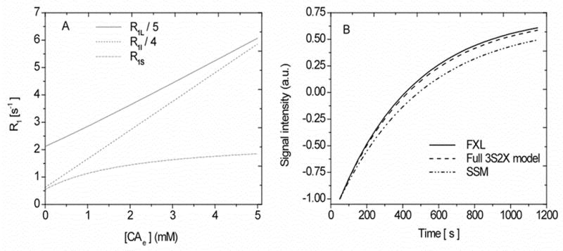
2A: Graph of simulated results of the analytical longitudinal relaxation rate constant R1 (e.g., R1S, I, L) as a function of the interstitial CA concentration [CAe] in a 3S2X model. Equation [A1] given in the Appendix was used to construct these curves. 2B. Simulated signal intensity time course curves at 0.95 mM Gd-DTPA in interstitial CA concentration for the LL imaging sequence and with tissue parameters ub= 0.02 and kbe = 2.0 s−1. The lower curve, labeled SSM, demonstrates the recovery of the longest component of longitudinal magnetization, sometimes used in previous studies (10,11) as the only component. The contribution of the components R1I and R1L on a signal that evolved 3S2X model, which were ignored in the SSM, can be seen. Model parameters values are listed in Table 1.
Figure 2B shows the time course of a simulated signal constructed for FXL (Equation [19]), full 3S2X model (Equation [16]) and a phenomenological curve, labeled SSM, which considers only the R1s component of Equation [16], a component that evolves from the 3S2X model but does not, as the graph shows, accurately reflect the true signal evolution in a typical LL experiment conducted in our laboratory at 7T. These curves were constructed using the LL imaging sequence employed here: number of sampling points (N) = 24, interexcitation time (τ) = 50 ms, tip angle (θ) = 18° at 0.95 mM of interstitial CA concentration with model parameters as in Figure 2A. The contribution of the R1I and R1L components can be seen on the full exchange model in comparison to the phenomenological model, SSM. While Figure 2B was generated from a 3S2X model, it bears a strong resemblance in signal behavior to that of Buckley’s Figure 6 (15), although that figure was generated using a 2SX model.
Figure 6.

Families of the plots obtained with the multi-time, graphical method of Patlak in a 3S2X model with the ordinate equal to and the abscissa equal to the efflux-corrected term , which is often referred to as ‘stretch time’ when the CA is injected as a bolus. 6A: With Ktrans = 0.01, 0.005, and 0.00125 min−1; top to bottom) and ub = 0.02. 6B: With blood water fractions, ub, set as 0.06, 0.04, and 0.01 (top to bottom) and Ktrans = 4 × 10⁻³ min−1. 6C: With the transendothelial rate of influx, kbe, varied from 10 to 2 to 0.5 s−1(top to bottom), Ktrans = 5 × 10⁻³ min−1, and ub = 0.05. 6D: Rate of exchange across parenchymal cell membrane set at either 10, 2, or 0.5 s−1 (top to bottom), Ktrans = 3 × 10⁻³ min−1, and ub = 0.03. The other parameters of this modeling are listed in Table 1.
Figure 3 displays the response of R1 to changes in tissue concentration under a range of conditions typical of those experienced in DCE studies. The temporal evolution of a LL signal was calculated using all the kernels of the relaxation rates (short, intermediate, and long) and their associated fractional populations in a 3S2X model. As before, the model was particularized to our LL experiment (N = 24, τ = 50 ms, and θ = 18°) with model parameters listed in Table 1.
Figure 3.

Simulated relaxation rate of tissue water protons (R1) versus tissue concentration of the contrast agent ([CAt]) in a 3S2X model. The curves were constructed with model parameters as follows: ub = 0.05, kbe = 5.0 s−1 and ui = 0.8, kie = 1.81 s−1. 3A: Simulated with the CA distributed only in the plasma compartment. The asterisk corresponds to the peak tissue CA concentration in the experimental condition. 3B: Simulated with the CA distributed in the blood and interstitial spaces. 3C: Families of simulated R1 curves for different values of kbe (10, 2, and 0.5 s−1; top to bottom). 3D: Families of simulated R1 curves for different values of kie (10, 2, and 0.5 s−1; top to bottom). The other parameters used in the modeling are given in Table 1.
Figure 3A shows, for an entirely intravascular CA, the relationship between LL estimates of the R1 of tissue water protons versus [CAt]. In this setting, R1 curves were constructed using a large volume fraction for blood water (ub = 0.05), kbe = 5.0 s−1, and cellular parameters: ui = 0.8 and kie = 1.81 s−1 with other model parameters as given in Table 1. The CA concentration in plasma [CAp] was varied up to 20.0 mM. Initially, R1 increases a nearly linear manner with [CAt] but curves concave at higher concentrations. Across the range plotted, the model data deviate about 15% (R1e = 0.5 s−1), 6.0% (R1e =10.0 s−1), and 10.0% (R1e = 20.0 s−1) from a linear relationship. As the R1 curve passes from its minimum to maximum, the exchange regimes across the abscissa [CAt] move from FXL to SXL. The relaxographic transvascular shutter speed |R1b − R1e| rapidly increases and exceeds the sum of the equilibrium rates of blood-tissue exchange, kt, ~ 6.67 s−1 around 3.20 mM of [CAp] and becomes effective in the upper half of [CAt]. It must be mentioned here that the range of this plot runs far beyond the usual experimental conditions. The asterisk on the plot points to the maximum value of CA concentration in plasma water that might be expected in most DCE studies; it should be concluded that the relationship between [CAt] and R1 is linear under most experimental conditions.
Figure 3B shows the LL estimates of R1 of tissue water protons versus [CAt] acquired with model data of Figure 3A when interstitial concentration was varied up to 5 mM. The model is constructed as if equilibration of the CA had take place between the blood and interstitial space. With increasing interstitial CA concentration, cellular exchange regimes vary from FXL to SXL. The difference in the longitudinal relaxation rates, |R1e − R1i|, exceeds kc at 2.75 mM of [CAe] and becomes effective in the upper half of the [CAt] range. The best fitted line to model data of R1 versus [CAt] yielded deviation about 15%, 7%, and 13%, respectively, at the lower (R1e = 0.5 s−1 ), middle (R1e =10.0 s−1), and upper (R1e = 20.0 s−1) points. Accordingly, the LL experiment predicted a nearly linear response between the R1 of tissue water protons and [CAt] in a 3S2X model.
In Figure 3C and 3D, the effects of varying the rates of exchange across the microvascular endothelium, kbe, (3C), and the membranes of parenchymal cells, kie (3D), on R1 are illustrated as a function of total tissue concentration. The rates of water exchange for kbe and kie (e.g., 10, 2.0 and 0.5 s−1: top to bottom) span the range for most tissue types. Figure 3C (ub = 0.05, ui = 0.8, and kie = 1.81 s−1) and D (ub = 0.05, kbe= 5.0 s−1, and ui = 0.8) were constructed with the model parameters used in Figs. 3A and B. The R1 curves under varying rates of water transfer become distinct in the upper region compared to the lower region of [CAt]. Across this rather wide range of tissue concentrations, the variation of kbe, again across a wide range of values (kbe = 2.0 s−1 (19) and kie = 1.81 s−1 (29) for normal brains) changes the slopes of line by 13%, and that of kie by 16%, respectively. This degree of variation would probably not be detectable under most experimental conditions.
Continuing our focus on the relation between tissue concentration and R1, we constructed a model of CA concentration in tissue in a moderately leaky vascular bed. Figure 4 shows the CA plasma concentration time-course of an experimentally measured [CAp(t)] (left ordinates) and the total CA tissue concentration [CAt(t)] (right ordinates) curves. The AIF is that of an intravenous (i.v.) bolus injection standard dose of 0.08 mmol/kg (body weight) of Gd-DTPA (27). The [CAt] time course was generated using the AIF and a CA transfer rate constant Ktrans = 0.002 min−1 and Equation [23] and associated expressions for ub = 0.02. These model concentrations were then used to investigate the relationship between R1 and tissue [CAt] with Look-Locker measurements of R1 as estimates of the latter.
Figure 4.
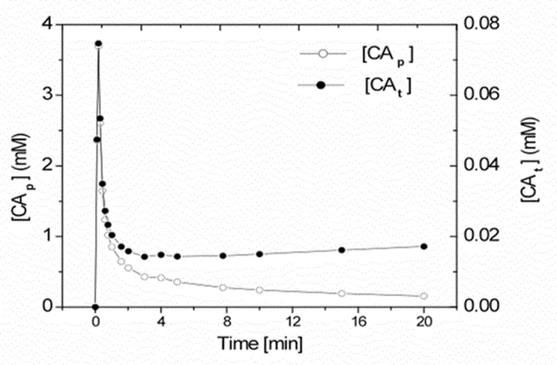
The time-course of plasma CA concentration ([CAp]; open circles) and total tissue CA concentration ([CAt]; filled circles). The latter, [CAt], was calculated using Equation [23] with Ktrans = 2 × 10⁻³ min−1 and ub = 0.02. The other model parameters are listed in the Table 1. This [CAp] concentration-time curve was used to generate Figures 5 and 6.
Given the concentration-time behavior of Figure 4, what can be expected of changes in R1? The R1b(t) and R1e(t) (e.g., Equations [8] and [9]) time-course curves were generated using an AIF and Equation [22], respectively, with ℜ = 4.2 mM−1s−1. The arterial hematocrit (Hct) was set to 0.5. Under this condition, the MR signal of the LL experiment (e.g. = 24, τ = 50 ms, and θ = 18°) was generated from the components of the longitudinal relaxation rate constants R1S, I, L, and the fractional populations in a 3S2X model. Then R1 was estimated as described in the preceding paragraphs according to Equation [19] from a signal obtained from Equation [16]. When the data is normalized so that the peak concentrations are plotted at the same ordinate distance, there clearly is a visual difference between tissue concentration and estimates of tissue concentration by ΔR1.
In Figure 5A, the normalized values of ΔR1 (open circles) predicted by the LL experiment conducted at 7T and the voxel CA concentration (filled circles) as a function of time are plotted for the case of an entirely intravascular CA in a 3S2X model. The two traces were normalized by setting the 20 min time point on the ordinate at the same graphical distance from zero for both. N.B.: the time scales of the two curves are offset, as indicated on the top and bottom abscissa labeling. It should be clear that the peak amplitude of the MRI estimate of tissue concentration when there is no CA leakage is smaller than the true peak, thus demonstrating the effect of restricted water exchange at the highest concentrations of CA.
Figure 5.

5A: Concentration-time plot of the change in the relaxation rate of tissue water protons (ΔR1; open circles) and tissue CA concentration (filled circles) for the case of all of the CA in blood. ub = 0.02. 5B: Concentration-time plot of ΔR1 (open circles) and tissue CA concentration (filled circles) for an entirely extracellular CA; this was modeled with Equation [22], Ktrans = 4.0 × 10⁻³ min−1 and ub = 0.02. 5C: Concentration-time plot of ΔR1 (open circles) and tissue CA concentration (filled circles) for the combined plots of 3A and 3B. The other model parameters values are listed in the Table 1. In 5C, the effect of the different apparent relaxivities of CA between blood and interstitium should be noted. While the component ΔR1’s track very closely with tissue concentration in their respective compartments, the combination does not.
In Fig 5B, the left and right ordinates demonstrate the change in the relaxation rate ΔR1 of the protons of tissue water (open circles) and tissue concentration [CAt] (filled circles), constructed from Equation [22], with Ktrans = 4.0 × 10⁻³ min−1 in a 2SX model. Here, it can be seen that the two estimates of concentration track each other very well. Certainly, any differences would be lost if MRI experimental SNR were in the range (e.g., 25:1) of what is usually achievable. Thus, despite figure 4, there appears to be a fairly good linearity in signal response when the blood and tissue components are considered separately.
Figure 5C plots ΔR1 (open circles, left ordinates) and [CAt] (filled circles, right ordinates), demonstrates the time behavior in a model of CA with leaky microvessels and includes both the blood and extracellular compartments gathered from Equation [23], when Ktrans = 4.0 × 10⁻³ min−1. Other model parameters were: ub = 0.02, kbe = 2.0 s−1, ui = 0.8 and kie = 1.81 s−1. In general, R1 as a function of time, when it is considered that CA resides only in the blood compartment or is equilibrated between the latter and the interstitial compartments, is well correlated with tissue concentration except at very high blood concentrations. Of note, the apparent relaxivity (the proportionality constant), however, differs among the compartments. Additionally, the apparent relaxivity for a given compartment will vary with water exchange rates and compartment size. This point has been repeatedly underscored in the development of the SSM (7,9,11–14), but the underlying linearity of the R1 response has not been as well represented using the appropriate boundary conditions for MR pulse sequences.
What then is the consequence of both the underlying linearity in concentration and the differences in apparent relaxivities? One of the better ways to examine this question is to utilize a method that is inherently linear, since it allows the examination of the model-generated response for nonlinearities. We chose the extended Patlak graphical method (2,5), which linearizes the concentration-time curve when there is appreciable brain-to-blood backflux of the CA (nonzero kb). Figure 6 shows a number of plots of concentration-time curves in tissue using the extended Patlak Graphical method (model 3 of Ewing et al (5)) constructed from Equation [24]. Using a 3S2X model, the influences of the vascular parameters Ktrans, ub, and the rates of water proton exchange kbe and kie on the Patlak plots are illustrated. As in the extended Patlak method, the quantity is the Patlak ordinate and efflux-corrected arterial time integral forms the abscissa. The quantity Ktrans is estimated from the slope of the plot, while fractional vascular volume is estimated from its intercept at x = 0.
In Figure 6A, the extended Patlak plot is produced for a range of blood-to-tissue transfer rate constants Ktrans (e.g., 0.01, 0.005, and 0.00125 min−1: top to bottom), to examine the systematic errors in estimates of Ktrans in a 3S2X model. In this setting, ub = 0.02 and kbe = 2.0 s−1, ui = 0.8 and kie = 1.81 s−1, and other model parameters given in Table 1 were used. The range of Ktrans spans the range for Gd-DTPA in most tissue types. For this range of Ktrans, the slopes vary by 87%, high to low, whereas the estimates of Ktrans vary about 4% from the true values; systematic errors in Ktrans are, thus, negligible. Contrariwise, the volume of intravascular water (i.e., the blood water space) is underestimated by as much as 56% compared to the true value.
Figure 6B shows how the Patlak plot behaves under a variation in the blood water fractions ub (e.g., 0.06, 0.04, and 0.01: top to bottom) in a 3S2X model. In this setting, the influx rate of protons linked to water (kbe = 2.0 s−1), intracellular parameters (ui = 0.8 and kie = 1.81 s−1), and model parameter listed in Table 1 were used. This range of ub is valid for many tissue types. To illustrate the effects of leakage, Ktrans was set to 4 × 10⁻³ min−1. The curves are distinct, differing in ub and with virtually identical slopes that vary by less than 3%. The volume of intravascular water is again underestimated by as much as 60% compared to the true value.
Figure 6C shows the influence of different rates of the transendothelial influx of water protons on the extended Patlak plot. The values of kbe (e.g., 10, 2, and 0.5 s−1: top to bottom) span values that model a highly permeable vasculature to that of a moderately restricted one. In this setting, Ktrans = 5.0 × 10⁻³, ub = 0.05, intracellular parameters (ui = 0.8 and kie = 1.81 s−1), and the model parameter listed in Table 1 were used. It can be seen that the curves are indistinguishable and slopes of the curves are nearly identical, varying by less than 1%. The estimated Ktrans differs by about 2% from the true value while ub varies by 58%. This result suggests that in the LL experiment the effect of intermediate transendothelial water exchange will have a negligible effect on the estimate of Ktrans and possibly a strong effect on vb, depending upon the tissue type.
Figure 6D illustrates how the rates of water proton exchange across parenchymal cell membranes, with kie varying from highly permeable to slightly restricted, in the 3S2X model influence Patlak plots of the data. In this setting, ub = 0.03 and kbe = 2.0 s−1, intracellular parameters (ui = 0.8 and kie = 1.81 s−1), and the model parameter listed in Table 1 and Ktrans = 3.0 × 10⁻³ min−1 were used. Under these conditions, the slopes of the curves and the estimates of Ktrans varied less than 1%. This result demonstrates the very small effect of a variation in water exchange cellular membranes has on the Patlak plot estimation of Ktrans.
Discussion
An analytical equation describing the evolution of magnetization for tissue water protons was formulated for the LL experiment via the Bloch–McConnell formalism using a 3S2X model, incorporating all three components of the longitudinal relaxation rates (e.g., short, intermediate, and long) and their associated fractional populations. A wide range of plasma and extracellular fluid concentrations of CA was considered, and signal associated with a LL experiment (N = 24 points, τ = 50 ms, θ = 18°) was generated. We were most interested in the relationship between the longitudinal relaxation rate of tissue water protons and tissue CA concentration, especially how a monoexponential summary of longitudinal signal recovery, R1, would be affected by the finite rate of equilibrium intercompartmental water exchange under the conditions of a typical DCE study. Thus, we have not considered the blood inflow effects in this study (16).
The results of Figure 3 illustrate a very important point: under a wide range of typical experimental conditions, a monoexponential estimate of R1 scales nearly linearly with [CAt]. It should be understood, however, that R1 as a measure of the CA concentration in the microvasculature is less linear (Figure 3A) than as a measure of the interstitial CA concentration (Figure 3B), although not strongly so. This is because a standard dose of 0.08 mmol/kg Gd-DTPA will result in a peak plasma concentration of about 3.7 mM (Figure 4: top), and the corresponding peak R1 can reach about 16.0 s−1. On the other hand, at the peak value of 0.77 mM of [CAe], the corresponding R1 is about 4.0 [sec−1] when Ktrans = 0.02 min−1. At very high concentrations of CA, the slope of the relationship between R1 and [CAt], i.e. the CA’s longitudinal relaxivity, varies with the rates of exchange across the endothelium and cellular membranes over the range of highly to moderately restricted microvascular permeability (e.g., top to bottom) in Figure 3C and D, respectively. Qualifying this, the deviations are relatively small even at very high concentrations and might easily be missed under typical experimental conditions with lower signal-to-noise.
The plots of data using the extended Patlak Graphical method are most revealing of the systematic behavior of the recovery of the longitudinal magnetization of tissue water protons when CA is limited to one or two compartments. Under typical experimental conditions, the cellular exchange regime moves from FXL to FXR to SXL. If the boundary conditions are properly modeled and all three components of recovery are taken into account, it is clear that water exchange across parenchymal cell membranes does not strongly influence the estimation of the influx transfer constant of the CA. On the other hand, if water exchange across the microvascular wall is moderately restricted as in normal brain, the blood water volume will be underestimated.
To investigate the effects of equilibrium intercompartmental water exchange kinetics on R1, this study mainly focused on the LL experiment. Water exchange times at the boundaries of the blood and intracellular compartments are about 500 ms and 550 ms, respectively, whereas the LL inter-echo sampling time scale, τ, is much smaller. On the other hand, the total acquisition time (e.g., 1200 ms) is much longer than the residence time of water molecules in either blood or intercellular fluid. It appears that, if the selected experimental time is long enough in comparison to the pre-exchange lifetime, a multipoint technique with an extended and repeated sampling may average the intercompartmental exchange of water protons under many conditions.
In all normal cerebral tissue as well as brain tumors, contrast materials are confined to the blood and extracellular space, whereas about 75% of the tissue water is intracellular. In the cerebral tumors, the change in the tumor volume affects on the water diffusion (32). Often the tissue studied by MRI and used for comparison in this study is a cerebral tumor, which has a highly permeable microvascular wall in contrast to normal brain. It appears highly probable that the exchange of water across tumor microvessels is more rapid than that across the surrounding normal vasculature. If this is the case, one can expect a general underestimation of blood water volume in normal brain parenchyma, and possibly in the ‘normalized’ vasculature of the tumor but a correct estimate of blood volume in the part of the tumor with highly permeable microvessels.
This study is not without limitations because several assumptions were made in the simulation. Probably the most restrictive set of assumptions involve the particularization to a 24-echo LL inversion-recovery experiment with 50 ms echo spacing and 18° tip-angle. However, we have investigated other experimental conditions, namely a 100 ms echo spacing, and/or a doubling of number of points. Generally, these variations in experimental condition do not change the results reported here by more than 1% in estimates of the transfer constant where as intercept vary within 5%, when Ktrans = 5.0 × 10⁻³ min−1 and ub = 0.03. Another restriction is the specification of 7 Tesla with its longer tissue T1’s, and lower CA relaxivities. Blood inflow effects were not considered, the pre-contrast blood and extracellular R1’s were set equal, and the CA relaxivities in the two compartments were set equal and assumed constant, although CA relaxivity may vary with macromolecular content (27) by as much as 30%. However, this latter variation simply changes the apparent relaxivity of the CA, and since the modeling covers a wide range of transcellular water exchange rates, which also changes the apparent relaxivity of the CA, variations in CA relaxivity with macromolecular content are probably covered by the modeling. We assumed that T*2 effects were negligible at these echo times. Notwithstanding these limitations, a clear picture evolves from this modeling: the systematic errors of the SM are likely to appear first in the underestimation of blood water volume. Only in tissue with extremely leaky microvessels and consequent high interstitial concentrations of CA will a serious underestimation of Ktrans begin to appear. Since the microvessels in this case will need to be extremely leaky, the practical consequences of an underestimation of Ktrans may not be important.
This kind of modeling with a full 3S2X treatment and correct boundary conditions needs to be extended to other, more clinically relevant field strengths and to more the widely employed short-TR gradient-echo sequences commonly used in clinical DCE determinations. An important first step toward this goal has been made and recently presented in abstract by those investigators who have pioneered the SSM (33).
Conclusion
We conclude that the analytic results of this study in a 3S2X model establish a nearly linear relationship between tissue CA concentration for a monoexponential estimate of R1 measured by a LL technique. Therefore, under many conditions, LL estimates of Ktrans will yield approximately unbiased estimates (within 4%) of that parameter in most tissues. On the other hand, it is likely that the volume of blood water in the field of observation can be significantly underestimated (as much as 60%), especially in normal brain tissue.
Acknowledgments
R01 CA135329-01: MRI Biomarkers of Response in Cerebral Tumors, RO1 HL70023-01A1 MRI Measures of Blood Brain Barrier Permeability
Symbols and Abbreviations
- R10b
Longitudinal relaxation rate of the intravascular space without CA
- R10e
Longitudinal relaxation rate of the extracellular space without CA
- R1b
Longitudinal relaxation rate of the intravascular space
- R1e
Longitudinal relaxation rate of the extracellular space
- R1i
Longitudinal relaxation rate of the intracellular space
- R*2
Effective transverse relaxation rate
- R1S
Shorter longitudinal relaxation rate of water protons’
- R1I
Intermediate longitudinal relaxation rate of water protons’
- R1L
Longer longitudinal relaxation rate of water protons’
- R*1
Effective Longitudinal relaxation rate of tissue water protons’
- R1
Longitudinal relaxation rate of tissue water protons’
- □
Longitudinal relaxivity of water protons’
- kbe
Rate of exchange of water protons’ from intravascular to extracellular space
- kie
Rate of exchange of water protons’ from intra- to extracellular space
- keb
Rate of exchange of water protons’ from extra- to intravascular space
- kei
Rate of exchange of water protons’ from extra- to intracellular space
- p1
Population fraction associated with longitudinal relaxation rate R1S
- p2
Population fraction associated with longitudinal relaxation rate R1I
- p3
Population fraction associated with longitudinal relaxation rate R1L
- ub
Intravascular water content fraction
- ue
Extracellular water content fraction
- ui
Intracellular water content fraction
- θ
Flip angle
- τ
Sampling interval time
- CAp
Plasma CA concentration
- CAe
Extracellular CA concentration
- CAt
Tissue CA concentration
- Ktrans
Blood to tissue CA transfer constant
- kb
Tissue to blood CA transfer constant
- 3S2X
Three site two exchange
- AIF
Arterial input function
- FXL
Fast exchange limit
- FXR
Fast exchange regime
- SXL
Slow exchange limit
Appendix
The following are the short, intermediate, and long longitudinal relaxation rate constants of a 3S2X model defined in the text:
| [A1] |
The relaxation rates are computed through the following relation:
| [A2] |
The following condition: R2 < Q3, is for the three different real roots of eigenvalues.
where
| [A3] |
| [A4] |
with
| [A5] |
References
- 1.Crone C. The permeability of capillares in various organs as determined by use of the ‘indicator diffusion’ method. Acta physiol Scand. 1963;58:292–305. doi: 10.1111/j.1748-1716.1963.tb02652.x. [DOI] [PubMed] [Google Scholar]
- 2.Patlak CS, Blasberg RG. Graphical evaluation of blood-to-brain transfer constants from multiple-time uptake data. Generalizations J Cerebral Blood Flow Metab. 1985;5(4):584–590. doi: 10.1038/jcbfm.1985.87. [DOI] [PubMed] [Google Scholar]
- 3.Patlak CS, Blasberg RG, Fenstermacher JD. Graphical evaluation of blood-to-brain transfer constants from multiple-time uptake data. J Cerebral Blood Flow Metab. 1983;3(1):1–7. doi: 10.1038/jcbfm.1983.1. [DOI] [PubMed] [Google Scholar]
- 4.Tofts P, Kermode A. Measurement of the blood–brain barrier permeability and leakage space using dynamic MR imaging. 1. Fundamental concepts. Magn Reson Med. 1991;17(2):357–367. doi: 10.1002/mrm.1910170208. [DOI] [PubMed] [Google Scholar]
- 5.Ewing JR, Brown SL, Lu M, Panda S, Ding G, Knight RA, Cao Y, Jiang Q, Nagaraja TN, Churchman JL, Fenstermacher JD. Model selection in magnetic resonance imaging measurements of vascular permeability: Gadomer in a 9L model of rat cerebral tumor. J Cerebral Blood Flow Metab. 2006;26(3):310–320. doi: 10.1038/sj.jcbfm.9600189. [DOI] [PubMed] [Google Scholar]
- 6.Donahue KM, Burstein D, Manning WJ, Gray ML. Studies of Gd-DTPA relaxivity and proton exchange rates in tissue. Magn Reson Med. 1994;32(1):66–76. doi: 10.1002/mrm.1910320110. [DOI] [PubMed] [Google Scholar]
- 7.Landis C, Li X, Telang F, Molina P, Palyka I, Vetek G, Springer C., Jr Equilibrium transcytolemmal water-exchange kinetics in skeletal muscle in vivo. Magn Reson Med. 1999;42(3):467–478. doi: 10.1002/(sici)1522-2594(199909)42:3<467::aid-mrm9>3.0.co;2-0. [DOI] [PubMed] [Google Scholar]
- 8.Labadie C, Lee JH, Vetek G, Springer CS., Jr Relaxographic imaging. J Magn Reson B. 1994;105:99–112. doi: 10.1006/jmrb.1994.1109. [DOI] [PubMed] [Google Scholar]
- 9.Landis CS, Li X, Telang FW, Coderre JA, Micca PL, Rooney WD, Latour LL, Vetek G, Palyka I, Springer CS., Jr Determination of the MRI contrast agent concentration time course in vivo following bolus injection: effect of equilibrium transcytolemmal water exchange. Magn Reson Med. 2000;44(4):563–574. doi: 10.1002/1522-2594(200010)44:4<563::aid-mrm10>3.0.co;2-#. [DOI] [PubMed] [Google Scholar]
- 10.Yankeelov TE, Rooney WD, Huang W, Dyke JP, Li X, Tudorica A, Lee JH, Koutcher JA, Springer CS., Jr Evidence for shutter-speed variation in CR bolus-tracking studies of human pathology. NMR in Biomedicine. 2005;18(3):173–185. doi: 10.1002/nbm.938. [DOI] [PubMed] [Google Scholar]
- 11.Yankeelov TE, Rooney WD, Li X, Springer CS., Jr Variation of the relaxographic “shutter-speed” for transcytolemmal water exchange affects the CR bolus-tracking curve shape. Magn Reson Med. 2003;50(6):1151–1169. doi: 10.1002/mrm.10624. [DOI] [PubMed] [Google Scholar]
- 12.Li X, Rooney WD, Springer CS., Jr A unified magnetic resonance imaging pharmacokinetic theory: intravascular and extracellular contrast reagents. Magn Reson Med. 2006;54(6):1351–1359. doi: 10.1002/mrm.20684. [DOI] [PubMed] [Google Scholar]
- 13.Li X, Huang W, Morris EA, Tudorica LA, Venkatraman ES, Rooney WD, Tagge I, Wang Y, Xu J, Springer CS., Jr Dynamic NMR effects in breast cancer dynamic-contrast-enhanced MRI. Proc Natl Acad Sci USA. 2008;105(46):17937–17942. doi: 10.1073/pnas.0804224105. [DOI] [PMC free article] [PubMed] [Google Scholar]
- 14.Huang W, Li X, Morris EA, Tudorica LA, Venkatraman ES, Rooney WD, Tagge I, Wang Y, Xu J, Springer CS., Jr The MR shutter-speed discriminates vascular properties of malignant and benign breast tumors. Proc Natl Acad Sci USA. 2008;105(46):17943–17948. doi: 10.1073/pnas.0711226105. [DOI] [PMC free article] [PubMed] [Google Scholar]
- 15.Buckely DL, Kershaw LE, Stanisz GJ. Cellular-interstitial water exchange and its effect on the determination of contrast agent concentration in vivo: Dynamic contrast-enhanced MRI of human internal obturator muscle. Magn Reson Med. 2008;60(5):1011–1019. doi: 10.1002/mrm.21748. [DOI] [PubMed] [Google Scholar]
- 16.Barbier EL, St Lawrence KS, Grillon E, Koretsky AP, Decorps M. A model of blood-brain barrier permeability to water: accounting for blood inflow and longitudinal relaxation effects. Magn Reson Med. 2002;47(6):1100–1119. doi: 10.1002/mrm.10158. [DOI] [PubMed] [Google Scholar]
- 17.McConnell HM. Relaxation rates by nuclear magnetic resonance. J Chem Phy. 1958;28:430–431. [Google Scholar]
- 18.Spencer RGS, Fishbein KW. Measurement of spin–lattice relaxation times and concentrations in systems with chemical exchange using the one-pulse sequence: breakdown of the Ernst model for partial saturation in nuclear magnetic resonance spectroscopy. J Magn Reson. 2000;142 (1):120–135. doi: 10.1006/jmre.1999.1925. [DOI] [PubMed] [Google Scholar]
- 19.Cao Y, Brown SL, Knight RA, Fenstermacher JD, Ewing JR. Effect of intravascular-to-extravascular water exchange on the determination of blood-to-tissue transfer constant by magnetic resonance imaging. Magn Reson Med. 2005;53(2):282–293. doi: 10.1002/mrm.20340. [DOI] [PubMed] [Google Scholar]
- 20.Herbest M, Goldstein JH. Cell water transport measurement by NMR. A three-compartment model which includes cell aggregation. J Magn Reson. 1984;60:299–306. [Google Scholar]
- 21.Brix G, Schad LR, Deimling M, Lorenz WJ. Fast and precise T1 imaging using a TOMROP sequence. Magn Reson Imaging. 1990;8(4):351–356. doi: 10.1016/0730-725x(90)90041-y. [DOI] [PubMed] [Google Scholar]
- 22.Look DC, Locker DR. Time saving in measurement of NMR and EPR relaxation times. Rev Sci Instrum. 1970;41(2):250–251. [Google Scholar]
- 23.Gelman N, Ewing JR, Gorell JM, Spickler EM, Solomon EG. Interregional variation of longitudinal relaxation rates in human brain at 3.0 T: relation to estimated iron and water contents. Magn Reson Med. 2001;45(1):71–79. doi: 10.1002/1522-2594(200101)45:1<71::aid-mrm1011>3.0.co;2-2. [DOI] [PubMed] [Google Scholar]
- 24.Ewing J, Knight R, Nagaraja T, Yee J, Nagesh V, Whitton P, Li L, Fenstermacher J. Patlak plots of Gd-DTPA MRI data yield blood-brain transfer constants concordant with those of 14C-sucrose in areas of blood-brain opening. Magn Reson Med. 2003;50(2):283–292. doi: 10.1002/mrm.10524. [DOI] [PubMed] [Google Scholar]
- 25.Kaptein R, Dijkstra K, Tarr CE. A single-scan fourier transform method for measuring spin-lattice relaxation times. J Magn Reson. 1976;24:295–300. [Google Scholar]
- 26.Kety SS. The theory and applications of the exchange of inert gas at the lungs and tissues. Pharmacol Rev. 1951;3:1–41. [PubMed] [Google Scholar]
- 27.Bagher-Ebadian H, Paudyal R, Nagaraja TN, Croxen RL, Fenstermacher JD, Ewing JR. MRI estimation of gadolinium and albumin effects on water proton. Neuroimage. 2010 doi: 10.1016/j.neuroimage.2010.05.032. [DOI] [PMC free article] [PubMed] [Google Scholar]
- 28.Nagaraja TN, Karki K, Ewing JR, Divine G, Fenstermacher JD, Patlak CS, Knight RA. The MRI-measured arterial input function resulting from a bolus injection of Gd-DTPA in a rat model of stroke slightly underestimates that of Gd-[14C]DTPA and marginally overestimates the blood-to-brain influx rate constant determined by Patlak plots. Magn Reson Med. 2010;63(6):1502–1509. doi: 10.1002/mrm.22339. [DOI] [PMC free article] [PubMed] [Google Scholar]
- 29.Quirk JD, Bretthorst GL, Duong TQ, Snyder AZ, Springer CS, Jr, Ackerman JJ, Neil JJ. Equilibrium water exchange between the intra- and extracellular spaces of mammalian brain. Magn Reson Med. 2003;50(3):493–499. doi: 10.1002/mrm.10565. [DOI] [PubMed] [Google Scholar]
- 30.Carreira GC, Gemeinhardt O, Beyersdorff D, Jorg Schnorr J, Taupitz M, Ludemann L. Effects of water exchange on MRI-based determination of relative blood volume using an inversion-prepared gradient echo sequence and a blood pool contrast medium. Magn Reson Imaging. 2009;27(3):360–369. doi: 10.1016/j.mri.2008.07.005. [DOI] [PubMed] [Google Scholar]
- 31.Press WH, Flannery BP, Teukolsky SA, Vetterling WT. Numerical recipe in C. Cambridge university press; 1987. [Google Scholar]
- 32.Kwee TC, Galban CJ, Tsien C, Junck L, Sundgren PC, Ivancevic MK, Johnson TD, Meyer CR, Rehemtulla A, Ross BD, Chenevert TL. Intravoxel water diffusion heterogeneity imaging of human high-grade gliomas. NMR Biomed. 2010;23(2):179–187. doi: 10.1002/nbm.1441. [DOI] [PMC free article] [PubMed] [Google Scholar]
- 33.Li X, Rooney WD, Varallyay CG, Gahramanov S, Muldoon LL, Goodman JA, Tagge IJ, Selzera AH, Pike MM, Neuwelt EA, Springer CS., Jr Dynamic-contrast-enhanced-MRI with extravasating contrast reagent: Rat cerebral glioma blood volume determination. J Magn Reson. 2010;206(2):190–199. doi: 10.1016/j.jmr.2010.07.004. [DOI] [PMC free article] [PubMed] [Google Scholar]