Multi-frequency characterization of the speed of sound and attenuation coefficient for longitudinal transmission of freshly excised human skulls

Abstract

For medical applications of ultrasound inside the brain, it is necessary to understand the relationship between the apparent density of skull bone and its corresponding speed of sound and attenuation coefficient. Although there have been previous studies exploring this phenomenon, there is still a need to extend the measurements to cover more of the clinically relevant frequency range. The results of measurements of the longitudinal speed of sound and attenuation coefficient are presented for specimens of human calvaria. The study was performed for the frequencies of 0.27, 0.836, 1.402, 1.965 and 2.525 MHz. Specimens were obtained from fresh cadavers through a protocol with the Division of Anatomy of the University of Toronto. The protocol was approved by the Research Ethics Board of Sunnybrook Health Sciences Centre. The specimens were mounted in polycarbonate supports that were marked for stereoscopic positioning. Computer tomography (CT) scans of the skulls mounted on their supports were performed, and a three-dimensional skull surface was reconstructed. This surface was used to guide a positioning system to ensure the normal sound incidence of an acoustic signal. This signal was produced by a focused device with a diameter of 5 cm and a focal length of 10 cm. Measurements of delay in time of flight were carried out using a needle hydrophone. Measurements of effective transmitted energy were carried out using a radiation force method with a 10 μg resolution scale. Preliminary functions of speed of sound and attenuation coefficient, both of which are related to apparent density, were established using a multi-layer propagation model that takes into account speed of sound, density and thickness of the layer. An optimization process was executed from a large set of random functions and the best functions were chosen for those ones that closest reproduced the experimental observations. The final functions were obtained after a second pass of the optimization process was executed, but this time using a finite-difference time-difference solution of the Westervelt equation, which is more precise than the multi-layer model but much more time consuming for computation. For six of seven specimens, measurements were carried out on five locations on the calvaria, and for the other specimen three measurements were made. In total, measurements were carried out on 33 locations. Results indicated the presence of dispersion effects and that these effects are different according to the type of bone in the skull (cortical and trabecular). Additionally, both the speed of sound and attenuation showed dependence on the skull density that varied with the frequency. Using the optimal functions and the information of density from the CT scans, the average values (±s.d.) of the speed of sound for cortical bone were estimated to be 2384(±130), 2471(±90), 2504(±120), 2327(±90) and 2053(±40) m s⁻¹ for the frequencies of 270, 836, 1402, 1965 and 2526 kHz, respectively. For trabecular bone, and in the same order of frequency values, the speeds of sound were 2140(±130), 2300(±100), 2219(±200), 2133(±130) and 1937(±40) m s⁻¹, respectively. The average values of the attenuation coefficient for cortical bone were 33(±9), 240(±9) and 307(±30) Np m⁻¹ for the frequencies of 270, 836, and 1402, respectively. For trabecular bone, and in the same order of frequency values, the average values of the attenuation coefficient were 34(±13), 216(±16) and 375(±30) Np m⁻¹, respectively. For frequencies of 1.965 and 2.525 MHz, no measurable radiation force was detected with the setup used.

1. Introduction

Longitudinal ultrasound transmission through the human skull has been proposed for imaging (Fry et al 1974, Carson et al 1977, Smith et al 1979, Dines et al 1981, Ylitalo et al 1990), Doppler imaging (Bogdahn et al 1990, Tsuchiya et al 1991, Jones et al 2001, Lindsey et al 2010) and therapeutic purposes (Fry 1977, Hynynen and Jolesz 1998, Tanter et al 1998, Tobias et al 1987, Hynynen et al 2001, Behrens et al 2001, Kinoshita et al 2006). The human skull presents a complex heterogeneous medium for sound transmission due to the solid, multi-layered, liquid-filled and porous composition of this tissue. Nevertheless, the attractiveness of using ultrasound for diagnostic and therapeutic purposes remains high due to its low-cost, portability and non-ionizing mechanism. For therapy, focused ultrasound surgery (FUS) has been proposed for the treatment of brain tumors (Fry 1977, Hynynen and Jolesz 1998, Tanter et al 1998, Tobias et al 1987), targeted drug delivery (Hynynen et al 2001), stroke treatment (Behrens et al 2001) and targeted antibody delivery (Kinoshita et al 2006). FUS efficiently concentrates the energy in a small region, while preserving surrounding structures. For therapy in the brain with FUS, the biggest challenge is to compensate the diffraction effects caused by the skull bone. When compared to soft tissue, the skull bone shows a faster longitudinal speed of sound and a higher density. When these facts are combined with the complex geometry of the skull cavity, the effective focusing of ultrasound becomes challenging (White et al 1968, Fry 1977, Hynynen and Jolesz 1998, Clement et al 2001, Pichardo and Hynynen 2007). However, this situation can be corrected using a multi-element device, where the phase of the signal in each element is adjusted to compensate for the diffraction effects (Hynynen and Jolesz 1998, Sun and Hynynen 1999, Clement et al 2000, Pernot et al 2003). The phase and amplitude of each element can be programmed using an invasive positioning of a hydrophone inside the brain (Smith et al 1986, Thomas and Fink 1996, Hynynen and Jolesz 1998, Tanter et al 1998, Clement and Hynynen 2002). Non-invasive correction can be done using sound propagation models, combined with detailed information of the skull, mostly provided by computer tomography (CT) scans (Sun and Hynynen 1999, Clement and Hynynen 2002, Aubry et al 2003). Previous reports have correlated the density information of the skull, which can be estimated from the CT voxels, with the speed of sound and attenuation (Connor et al 2002); this makes possible to achieve the required focusing in a non-invasive approach.

In this study, we extend the knowledge about the acoustic characteristics of the human skull for longitudinal sound transmission. Specifically, we present our findings for the speed of sound and attenuation coefficient for longitudinal sound propagation for frequencies ranging from 0.27 Hz to 2.525 MHz. Special attention was paid during the extraction and preconditioning of the human calvaria in order to minimize the possibility of any denaturalization caused by unknown influences. The spatial registration of the skull also demanded special attention to ensure the precise positioning during the measurements. Following the approach proposed previously (Connor et al 2002) to express the speed of sound in the skull bone as a continuous spline function of the density, functions of speed of sound and attenuation specific to each frequency are presented. This study covers an important spectrum of ultrasound frequencies that allows analysis of the potential dispersion effects of the skull bone.

2. Material and methods

2.1. Methodology

The goal of this study was to establish functions for the coefficients of attenuation and speed of sound, corresponding to the longitudinal sound propagation in human skull bone. The study was performed for the frequencies of 0.27, 0.836, 1.402, 1.965 and 2.525 MHz. Both the coefficient of attenuation and speed of sound were expressed as the functions of the apparent skull density obtained from CT scans. Experimental measurements were made to obtain the relative absorbed energy by the skull bone, under conditions of normal incidence of ultrasound transmission through a cross-sectional area of small dimensions. The delay caused by the skull bone in the propagation of an acoustic wave was also measured.

A multi-layered scheme of sound transmission for plane waves was used to model the ultrasound propagation through the skull bone. An optimization process was executed to establish a population of best-fitted functions of the attenuation and speed of sound that match the experimental measurements with the propagation model. A robust, but computationally more time-consuming model of sound propagation was used to corroborate the precision of the multi-layer model, where the information of density was specified at the voxel level rather than at the layer level. This robust model, which is based on the Westervelt equation (Hamilton and Blackstock 1998), helped to pre-select the best functions of the attenuation and speed of sound.

With this subset of pre-selected functions, the optimization process was executed again, but using the Westervelt equation to calculate the cost function. It was expected that the multi-layered model would be precise enough to provide a ‘first good guess’ and the more precise solution of the Westervelt equation would help to establish a more definitive relationship between the density and the speed of sound and attenuation.

2.2. Specimens

Seven human calvaria from adults were obtained through a research agreement with the Division of Anatomy of the University of Toronto. The protocol was approved by the Research Ethics Board of Sunnybrook Health Sciences Centre. No personal data were collected and specimens were identified by roman numbers from I to VII. Each specimen consists of the supra-orbital region of the skull, which includes bone from the frontal, parietal and occipital segments. The specimens were obtained initially fixed in 5% buffered formalin. After transportation from the Division of Anatomy to our laboratory, the specimens were immersed in 10% buffered formalin. As shown in figure 1, after removal of all surrounding soft tissue (scalp and dura-mater), each specimen was mounted in a polycarbonate frame with a length of 25 cm, width of 20 cm and thickness of 1.27 cm. The skull was placed inside a central perforation of 19 cm by 15.5 cm. Each skull was secured to the support using four 4 mm diameter nylon screws placed in the anterior, posterior, left and right extremes of the skull cap. Each frame was marked with six holes of diameter 0.7 mm for stereoscopic positioning. As shown in figure 1, each frame has two gripping holes to clip tightly the support to the position system, which is described below. After their mounting on the frame, each skull cap was immersed in degassed water and put under vacuum at −0.7 MPa for 8 h. Still immersed in degassed water, specimens were imaged with a CT scanner (LightSpeed VCT, GE Healthcare, Chalfont St Giles, UK) using a bone kernel and voxel resolution and slice thickness of 0.625 mm.

Figure 1.

Top-view scheme of the setup used for the mounting of skulls. Each skull was attached to a polycarbonate support with four nylon screws. The support has two gripping holes used to mount the support in a positioning arm and has six small holes (shown with a ‘+’) with a diameter of 0.7 mm used for stereoscopic positioning. The small holes were made in pairs on the locations close to the corners of the support as follows: right-top, right-bottom and left-bottom.

A three-dimensional surface of the skull caps was reconstructed using an isosurface extraction algorithm (Wong and Heng 1998). Surface triangles belonging either to the internal or the external face of the skull were identified by the dot product between the normal vector of each triangle and a vector between the triangle center and a point located inside the skull cavity. A program with a graphical interface written in Matlab (R2009a, Mathworks, Natick, MA, USA) was used to locate the coordinates of the markers on the supports in the CT coordinate system. Figure 2 shows a slice of one of the skulls where one of the markers on the support is visible. Figure 3 shows a rendering of one of the skull caps, including its support frame, using an intermediate Cartesian coordinate system (ICS). The ICS was defined with its origin located on the bottom face of the support plate. The coordinates of the markers (holes) in the polycarbonate support were measured in the ICS with a caliper. Using the coordinates of the markers in the ICS and in the CT’s coordinate system, a matrix of translation–rotation was reconstructed (Horn et al 1988) to convert the coordinates of the surfaces of the skull to the ICS.

Figure 2.

Left: axial CT-slice of a skull and its polycarbonate support. Right: close-up of the region where one of the markers used for stereoscopic positioning is visible.

Figure 3.

Surface visualization of skull III in the independent coordinate system (ICS). The polycarbonate support is also shown. Once the triangulated surface was extracted in the CT’s coordinate system, the triangle coordinates were rotated–translated in the function of the position of the markers in the ICS and in the CT’s system. For illustration purposes, the figure shows a skull surface composed of only 5% the number of triangles used in the study.

2.3. Positioning system

A special arm was built to attach the polycarbonate frame to a manual 5° positioning system, which is composed of a three-directional Cartesian positioning system (A25 series, Velmex, Bloomfield, NY, USA) and two precision optical manual rotation stages (481-A, Newport, Irving, CA, USA). The rotation stages allow the rotation around the x and z axes of the ICS with a precision of 0.5°. The Cartesian positioning system has a resolution of 0.01 mm. The arm was located inside a large tank with dimensions large enough to allow the displacement and rotation of the specimen. The tank walls were covered with absorbent material (Neoprene 70 sheets with a thickness of 1.27 cm). Before each experiment, a polycarbonate frame with no central perforation and with markers at its center, matching the origin of the ICS, was used to calibrate the ICS and the coordinate system of the positioning arm (PCS).

A software tool with a graphical interface written in Matlab was used to guide the user to select a location on a given skull. Since the triangulation method also gives the normal vector of each triangle of the skull surface, the calculation of the incidence angle is straightforward through the use of the dot product between this normal vector and the acoustic axis, which in our case matches the z axis of the PCS. The software shows the average and standard deviation of the incidence angle over a cross-sectional surface area of 0.25 cm². The software allows the selection of a specific point on the skull surface, and it can rotate the skull around this point until reaching a desired incidence angle. The software shows coordinates in both the PCS and ICS. By using the ICS, the user can choose the desired point regardless of the correction required for the PCS. After calibration between the PCS and the ICS, the software indicates the required coordinates in the PCS and the required angle on the rotation stages.

2.4. Propagation model

Figure 4 shows the multi-layer model used to calculate the attenuation coefficient and the speed of sound under normal incidence conditions. Layers 1 and N + 1 are water and the inner layers 2 to N are considered solid. We assume that from the total energy sent by the transducer, a part of the energy is reflected back to the source, another part is attenuated by the skull and the remaining energy crosses the skull. An analytical model can be obtained to calculate the amplitude coefficient T for a plane wave that crosses a multi-layer propagation medium (Brekhovskikh and Godin 1990, Hayner and Hynynen 2001). This model is based on solving the potential of velocities and stresses at each interface. Coefficient T is complex to model changes in amplitude and phase of the wave reaching the layer N + 1. The calculation of the coefficient T for a multi-layered medium surrounded by water can be performed using (Folds and Loggins 1977)

Figure 4.

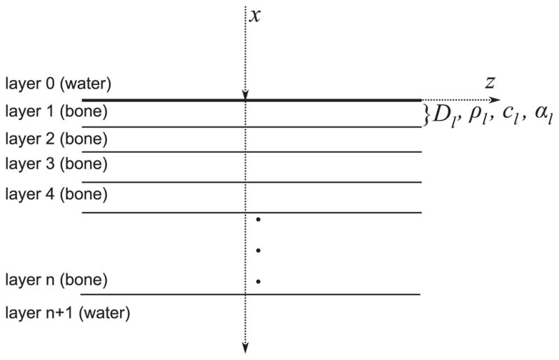
Multi-layer model used for sound propagation. A block of solid material, which is composed of n-layers, is surrounded by water (layers 0 and n + 1). Each layer has independent properties for thickness (D_n), density (ρ_n), speed of sound (c_n) and attenuation (α_n).

$$T=\frac{2Z_w}{(m_{2,2}+m_{3,3}+Z_w{m}_{2,3})Z_w+m_{3,2}},$$ (1)

where

$$m_{j,k}=A_{j,k}-\frac{A_{j,1}{A}_{4,k}}{A_{4,1}},$$ (2)

Z_w = ρ_wc_w is the acoustic impedance of water and A_j,k is a coefficient of the matrix for multiple transmission for the stress (S_x, S_z) and particle velocity (v_x, v_z) given by

$$\left[\begin{array}{c}{v}_x^N\\ v_z^N\\ S_z^N\\ S_x^N\end{array}\right]=\left[\begin{array}{cccc}{A}_{1,1}& A_{1,2}& A_{1,3}& A_{1,4}\\ A_{2,1}& A_{2,2}& A_{2,3}& A_{2,4}\\ A_{3,1}& A_{3,2}& A_{3,3}& A_{3,4}\\ A_{4,1}& A_{4,2}& A_{4,3}& A_{4,4}\end{array}\right]\left[\begin{array}{c}{v}_x^1\\ v_z^1\\ S_z^1\\ S_x^1\end{array}\right].$$ (3)

The matrix of coefficients A_j,k is obtained after the consecutive multiplication of the matrices of the sound transmission coefficients C_n of a given layer n to have

$$\left[\begin{array}{cccc}{A}_{1,1}& A_{1,2}& A_{1,3}& A_{1,4}\\ A_{2,1}& A_{2,2}& A_{2,3}& A_{2,4}\\ A_{3,1}& A_{3,2}& A_{3,3}& A_{3,4}\\ A_{4,1}& A_{4,2}& A_{4,3}& A_{4,4}\end{array}\right]=C_N{C}_{N-1}\cdots C_2.$$ (4)

Under normal incidence conditions, for a given layer n its corresponding matrix C_n(Folds and Loggins 1977) can be simplified to

$$C_n=\left[\begin{array}{cccc}-cos{\varsigma }_n{D}_n& 0& 0& -\text{i}\frac{{\varsigma }_{n}sin{\varsigma }_n{D}_n}{{\rho }_n\omega }\\ 0& cos{k}_n{D}_n& -\text{i}\frac{k_{n}sin{k}_n{D}_n}{{\rho }_n\omega }& 0\\ 0& -\text{i}\frac{{\rho }_n\omega sin{k}_n{D}_n}{k_n}& cos{k}_n{D}_n& 0\\ -\text{i}\frac{{\rho }_n\omega sin{\varsigma }_n{D}_n}{{\varsigma }_n}& 0& 0& -cos{\varsigma }_n{D}_n\end{array}\right],$$ (5)

where k_n and ς_n are the complex wave numbers for the longitudinal and shear transmission, respectively, of the layer n. D_n (m) and ρ_n (kg m⁻³) are, respectively, the thickness and density of the same layer. The form of the matrix C_n implies that all coefficients equal to zero remain as zero after the multiplication of C_n by C_n−1 and so on. Furthermore, coefficients ς_n disappear for the calculation of (1) since A_4,2 and A_4,3 are equal to zero. This situation makes that

$$m_{2,2}=m_{3,3}=A_{2,2},m_{2,3}=A_{2,3},m_{3,2}=A_{3,2},$$ (6)

which allows writing the equation of transmission (1) as

$$T=\frac{2Z_w}{(2A_{2,2}+Z_w{A}_{2,3})Z_w+A_{3,2}}.$$ (7)

It is important to note that (7) is consistent with the fact that under normal incidence conditions there is no transmission of sound for shear waves. The complex wave number k_n is given by

$$k_n=\frac{\omega }{c_n\left(1-\text{i}\frac{2{\alpha }_n{c}_n}{\omega }\right)}$$ (8)

where c_n (m s⁻¹) and α_n (Np m⁻¹) are the speed of sound and attenuation coefficient assigned to the layer n. A priori the values of the local coefficients c_n and α_n may be arbitrary or they can be a function of a structural composition. In this study, if a point in the space was identified as the skull bone, the values of c and α were considered as the functions of the density and will be denoted in the following as c_s(ρ) and α_s(ρ), respectively. The acoustic impedance of water Z_w was calculated with a density of 1000 kg m⁻³ and speed of 1483 m s⁻¹.

2.5. Density of skull

As shown in figure 5, the total number of layers and the skull density ρ_n was estimated from the CT dataset (Connor et al 2002) by the voxels identified as skull that were found following the acoustic axis. The value of ρ_n for each layer was assigned by the average values of the voxel on the acoustic axis and four surrounding voxels found in the same perpendicular plane where the central voxel was located. The center-to-center distance between voxels on the same perpendicular plane was set to the voxel spacing of the CT dataset (0.625 mm). The thickness D_n was set for all layers to 1/4 the voxel spacing of the CT dataset to allow a smooth transition. The total number of layers depended on the thickness of the skull bone, found at a given region of interest.

Figure 5.

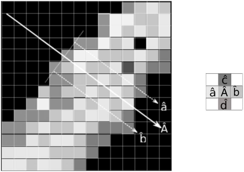
Reconstruction of layers for sound propagation from a CT scan. For illustration purposes, a fake close-up of the voxels of a section of skull bone from a CT slice is used where the white voxels represent high values of density. In the close-up, a simulated section of skull bone is shown where the dark voxels are water and the light gray voxels are bone material. The acoustic axis, shown by vector Â, is perpendicular to the surface of the skull bone. Four vectors (â, b̂, ĉ and d̂), which are parallel to Â, are used to reconstruct a perpendicular plan for a given location on Â.

The analysis of the profiles of the density paths covered by the sound transmission can help to identify the regions corresponding to each type of bone. Cortical bone is characterized by a higher density when compared to trabecular bone. It was expected that cortical bone would appear as two peaks in the density path, while trabecular bone would appear as a valley between the two peaks. This identification can help to isolate the behavior of the speed of sound and attenuation by the specific type of bone.

2.6. Error of function of attenuation

The transmitted power P_t of a plane wave crossing a solid layer under normal incidence conditions can be calculated by (Brekhovskikh and Godin 1990, Cheeke 2002, Hayner and Hynynen 2001)

$$P_t=P_0{TT}^{\ast },$$ (9)

where P₀ (W) is the acoustic power reaching the layer 1 in figure 4. T^* is the complex conjugate of the transmission coefficient T calculated with (7). In (9), T T^* indicates the ratio of the total absorbed energy P_t P₀⁻¹, which is expected to be less or equal to 1. We assume that we have an experimental measurement of P_t P₀⁻¹ that will be denoted in the following by P̂_t P̂₀⁻¹. For a given function α_s(ρ), the error η (in percentage) associated with that function and an experimental measurement can be expressed by

$$\eta =\left(\frac{{TT}^{\ast }}{{\widehat{P}}_t{\widehat{P}}_0^{-1}}-1\right)\times 100\%.$$ (10)

For each frequency f to be tested, we assume having a number of M experiments and the total least-squares error can be given by

$${\mathrm{\Xi }}_f=\frac{1}{M}\sum _1^M\eta {(m)}^2$$ (11)

where η(m) is the error associated with the m-measurement for a given function α_s(ρ). It was expected that there was a function α_s(ρ) that minimized Ξ_f. An optimization process (section 2.8) was executed to find the optimal α_s(ρ) for a given frequency.

2.7. Error of function of speed of sound

From a macroscopic point of view, the introduction of the skull bone between a source and an observation point makes an acoustic signal arrive with a delay δ (in seconds) when compared with the signal observed when the skull bone was absent. In a multi-layered model, δ can be estimated as the sum of delays caused by each layer. Consequently, δ can be expressed by

$$\delta =\sum _{n=2}^N\frac{D_n}{c_s(\rho )},$$ (12)

where c_s(ρ) is the speed of sound corresponding to a given layer n via the density of that layer. Similarly as for α_s(ρ), the error ε of a function c_s(ρ) associated with the measurement of the delay can be expressed by

$$\epsilon =(\widehat{\delta }-\delta )\omega ,$$ (13)

where δ̂ is the measured delay, and ε is given in radians, which makes the comparison of error between functions c_s(ρ) easier for different frequencies. Similarly for function α_s(ρ), we assume having a number of M experiments for each frequency f to be tested and the total square error can be given by

$${\mathrm{\Psi }}_f=\frac{1}{M}\sum _1^M\epsilon {(m)}^2$$ (14)

where ε(m) is the error associated with the m-measurement for a given function c_s(ρ).

2.8. Optimization algorithms

It was expected that for each frequency tested, there was a function α_s(ρ) that minimized the total error Ξ_f. It is an identical case for the speed of sound, as there was a function c_s(ρ) that minimized the total error Ψ_f. Each function followed a continuous cubic spline given by the minimization of (De Boor 2001)

$$\upsilon \sum _{j=1}^N{(X_j-X({\rho }_j))}^2+(1-\upsilon )\int {\left(\frac{{\text{d}}^{2}X}{\text{d}{\rho }^2}\right)}^2\text{d}\rho ,$$ (15)

where X is either c or α. X_j and ρ_j are the j-knots of the spline function, and υ is the weight for fitting closely the curve to the knots. As reported previously (Connor et al 2002), it is possible to represent the properties of the skull with a smooth and continuous function by setting υ = 0.99. For each frequency f tested, an optimization process was executed to find the set of knots that produced the function α_s(ρ) that minimized the square error Ξ_f. A similar process was executed to find the function c_s(ρ) that minimized the square error Ψ_f.

Each optimization process consisted of creating an initial population of 50 pseudo-random sets using a multiplicative random-number generator with the function RandStream(‘mcg16807’) of Matlab (R2009a, Mathworks, Natick, MA, USA) using seeds ranging from 1 to 50. Each set consisted of seven knots for ρ_j and seven knots for X_j. The choice of seven knots was established after a preliminary execution of the optimization process where the minimum number of knots was established. As suggested in Connor et al (2002), five knots are enough to describe a smooth transition of the functions of speed of sound. However, our results showed that increasing the number of knots to 7 helped to reduce the number of iterations required to converge to a feasible solution. A larger number of knots did not show up any improvement in the number of iterations.

The knots for ρ_j were uniformly distributed between 1000 and 3400 kg m⁻³. For the speed of sound, the knots were distributed between 1500 and 5500 m s⁻¹. For the attenuation, the knots were distributed between 10 and 500 Nepers m⁻¹. For each set of initial random knots, two algorithms for optimization were executed: constrained genetic (CG) and constrained sequential quadratic programming (CSQP). Both algorithms are available in Matlab. Genetic algorithms produce new sets pairing the best ‘mates’ and introduce some degree of mutation during pairing (Goldberg 1989). The constrained methods ensure that in every step of the optimization the new sets respect a specified set of rules. The CSQP algorithm uses a quasi-Newton method, where the evolution of the knots depends on the gradient between two sets where a small change has been introduced (Fletcher 1988). In principle, the CG is more susceptible to produce an optimal solution that is less dependent on the initial sets of coefficients. The CSQP algorithm depends greatly on the initial set, and it is assumed to find a set of knots that always produces a local minimum in the cost function. By providing a large population of initial sets, the opportunity for a CSQP-based method to find the optimal set of knots is maximized.

The genetic algorithm was executed with the function ga of Matlab with the option @mutationadaptfeasible for the genetic method. The stopping criteria were getting an incremental gain in the minimization or a change of the values of the knots less than 10⁻⁶; evolve up to 10⁴ generations, each generation with 30 sets. The CSQP method was denoted with the function fmincon. The stopping criterion was either a maximum number of iterations of 10⁶ or an incremental gain less than 10⁻⁶.

Since the attenuation and speed of sound were studied separately, for the estimation of α_s(ρ) the speed of sound was set using a function previously reported (Connor et al 2002). By doing this, the optimization process only adjusted the coefficients regarding the cost function of the attenuation. Similarly, for the optimization of the speed of sound, a constant value of attenuation was used, which was calculated using the transmitted energy and the thickness of the skull bone observed during experimentation (see section 2.9.1).

2.9. Experimental measurements

An in-house-manufactured air-backed transducer was used for the experiments. The transducer is made of gold-plated lead zirconate titanate (PZT) and is shaped as a spherical cap with a diameter of 5 cm and a focal length of 10 cm. Its central frequency is 0.254 MHz and passive electrical adaptation circuits were made for the frequencies of 0.27, 0.836, 1.402, 1.965 and 2.525 MHz. The device was positioned at the bottom of the water tank and the acoustic axis was aligned vertically. The transducer was excited by an electrical signal produced by a function generator (Wavetek 395, Fluke, Everett, WA, USA) and amplified with a gain of 50 dB with a wide-band linear amplifier (275LC-CE, Kalmus, Bothell, WA, USA).

2.9.1. Attenuation experiments

Figure 6 shows the setup used to estimate the ratio P_t P₀⁻¹ for the longitudinal attenuation coefficient in the skull. The transducer was located 12 cm below the skull interface, meaning that the cross-section area on the skull was located in the post-focal region. The internal face of the skull was positioned facing the transducer, making the sound cross from the internal to the external face of the skull. This orientation was chosen because the sound absorber is large enough to capture most of the sound crossing the skull. The absorber had a diameter of 8 cm and was positioned at approximately 2 cm over the external face of the skull. After considering the average thickness of the skull bone is 0.8 cm, the absorber was located around 15 cm from the transducer. The absorber is made of frayed polymer bristles, bundled so the closely packed tips acted as point scatters. These scatters deflect most of the energy into the brush, where it becomes absorbed (Hynynen 1993).

Figure 6.

(a) Positioning system and scheme of tank setup used to measure the attenuation coefficient in the skull. The analytical balance was placed on the top of a wood box (not shown in diagram) that surrounded the water tank. (b) Electronics setup used for the acquisition.

The sound absorber was attached using nylon wires to a 10 μg resolution analytical balance (PI-225D, Denver Instruments, Denver, CO, USA). The balance was mounted on a wood box that surrounded the water tank. The force applied on the acoustic absorber was recorded by a computer attached via RS-232 to the balance. The effective transmitted electrical power was monitored by a power meter (E4419B, Agilent, Palo Alto, CA, USA) coupled with the transmitted signal by a dual-directional coupler (Model 01575 Werlatone, Brewster, NY, USA). The reading of the power meter was captured by the computer via a GPIB interface, simultaneously with the reading of the balance. With the reading of effective electrical power and the applied force on the balance, the percentage of the transmitted energy E_t was calculated (Hynynen 1993).

For each location and frequency, five measurements were performed using an exposure with 3 s duration and 6 W effective electrical power. The power of 6 W was selected after preliminary experiments were performed with thermocouples (T-type) placed over a cross-sectional area of the parietal bone on the skull I. Several powers ranging from 4 to 12 W, with steps of 2 W, were tested with the exposure of 3 s at the highest frequency of 2.525 MHz. The transient temperature was recorded after ultrasound was turned off (TDS3012B, Tektronix, Beaverton, OR, USA). Powers of 10, 12 and 14 showed an increase of 0.5, 1.8 and 3.4 °C, respectively. Powers of 4, 6 and 8 W did not show any measurable increase of temperature. The power of 6 W was selected for measurements as a conservative choice that will minimize any internal heating of the skull bone.

For the absorption experiments, a waiting time of 30 s was used to allow cooling of the bone and absorber. Before each experiment on a given skull, a reference of the exerted force was performed for each frequency, with the absence of the skull, but with all supportive structures intact. These reference values were then used to calculate the percentage of the transmitted energy E₀ for each frequency under water-only conditions. If we assume that the sound absorber captured most of the acoustic energy, then it is possible to write the equity relationship by

$$\frac{{\widehat{P}}_t}{{\widehat{P}}_0}=\frac{E_t}{E_0}.$$ (16)

2.9.2. Speed of sound measurements

A time-of-flight setup was used to estimate the speed of sound in the skull. As shown in figure 7, the setup was essentially the same for the attenuation coefficient estimation, with the difference being that the absorber was removed and a 0.2 mm diameter PVDF needle hydrophone (SN 1378, Precision Acoustics, Dorchester, Dorset, UK) was positioned over the skull. The hydrophone was mounted on a miniature three-directional Cartesian positioning system (275LC, Edmund Industrial Optics, Barrington, NJ, USA), which was secured to one of the walls of the tank. An oscilloscope (TDS3012B, Tektronix, Beaverton, OR, USA) recorded the hydrophone signal that was previously adapted (DC1/253, Precision Acoustics, Dorchester, Dorset, UK) and filtered using a passive 5 MHz low-pass filter (BLP-5+, Mini-circuits, Brooklyn, NY, USA).

Figure 7.

(a) Scheme of a tank setup used to measure the speed of sound in the skull. The hydrophone was mounted on a miniature three-directional Cartesian positioning system (not shown in diagram). (b) Electronics setup used for the acquisition.

The hydrophone was positioned between 2 and 3 cm from the skull surface, and the acoustic axis was established by finding the location that produced the highest amplitude level of the signal. This procedure was followed for all selected locations on a given skull and for all frequencies. The final position of the hydrophone was the site that ensured that there was a signal strong enough for all locations and frequencies. Once the hydrophone location was chosen, the arm was locked to avoid any displacement.

The function generator triggered the oscilloscope and was programmed in the burst mode with 15 cycles and a repetition frequency of 10 Hz. The signal amplitude at the function generator was the same as the one used for the measurements of attenuation, which in a continuous mode would produce 6 W of electrical power. The signal acquired by the scope was transferred to a computer via a GPIB interface. When all the acquisitions were made for all frequencies, the skull was removed carefully while keeping the position of the hydrophone locked. Measurements without the skull were made again for each frequency. This procedure was repeated for each location on the skull and for each frequency.

The measured delay δ̂ was calculated using a semi-automatic program written in Matlab, where the user indicated the location in time of the beginning of the signals. The program calculated the delay that produced the maximum value in the cross-correlation of both signals. It also limited the time window from the beginning of the signal identified by the user to the time after the number of cycles used in experiments, which in our case was 15 cycles. The calculation of δ̂ considered the transmission of sound through a layered medium with different speeds of sound. This implies that the observed signal with a hydrophone arrives with a different phase when compared to a water-only reference signal. Strictly speaking, δ̂ can be expressed as δ̂ = φ · ω⁻¹, where |φ| can be larger than 2π. In practice, and under the conditions used in this study, the calculation of δ̂ was performed using an iterative loop where the cross-correlation value r was calculated between the reference signal s_w and a re-phased skull signal $s_s^{\ast }$, which was calculated with the expression

$$s_s^{\ast }={\text{FFT}}^{-1}(\text{FFT}(s_s)exp(\text{i}\phi )),$$ (17)

where s_s is the original signal with the presence of the skull and φ is the phase (in radians) to be tested. FFT and FFT⁻¹ are the direct and inverse fast Fourier transform, respectively. It was expected that the value of the correlation r was maximal for a given value of φ and a lag l between the s_w and $s_s^{\ast }$. The values of r and l were calculated with the function xcorr of Matlab (R2009a, Mathworks, Natick, MA). δ̂ was then calculated with the expression

$$\widehat{\delta }=l_{\text{opt}}+\frac{{\phi }_{\text{opt}}}{\omega },$$ (18)

where l_opt and φ_opt are the pair of required lag (in seconds) and phase that produces the maximum value of correlation r.

2.10. Theoretical validation of functions of speed of sound and attenuation

The multi-layer model used previously allowed the establishment of a population of candidate functions and a more robust model helped with the definitive selection of the best function per frequency. The Westervelt equation (Westervelt 1963) was selected to evaluate the propagation of sound with each one of the functions α_s(ρ) and c_s(ρ). This model takes the specific properties per voxel into consideration and the equation is given by

$$\frac{{\partial }^{2}p}{\partial z^2}-\frac{1}{c^2}\frac{{\partial }^{2}p}{\partial t^2}+\frac{\mu }{c^4}\frac{{\partial }^{3}p}{\partial t^3}+\frac{2\beta }{\rho c^4}\left[p\frac{{\partial }^{2}p}{\partial t^2}+{\left(\frac{\partial p}{\partial t}\right)}^2\right]-\frac{\partial p}{\partial z}·p\frac{\partial (ln\rho )}{\partial z}=0$$ (19)

where p is the pressure of the acoustic wave, and c ρ, μ and β are, respectively, the local coefficients of speed of sound, density, diffusivity and nonlinearity. For harmonic excitation, μ is related to the attenuation coefficient α with μ = 2αc³(2πf)⁻². A finite-difference time difference (FDTD) was used to solve (19) in cylindrical coordinates (Connor et al 2002). The solution of (19) is computationally more time consuming than the multi-layer model (three orders of magnitude). For example, the calculation of the sound transmission over a cross-sectional area of 0.25 cm² at a frequency of 270 kHz takes around 280 s, while the multi-layer model takes barely a fraction of second. The FDTD implementation takes advantage of multi-core technology using OpenMP and running with a computing node with 2 quad-core processors (Intel Xeon 5410). For higher frequencies, the difference is even higher; for 1402 kHz the calculation takes around 840 s, while the execution time with the multi-layer model remains less than a second.

The performance of each function α_s(ρ) and c_s(ρ) was measured by forward propagating, with (19) the real acoustic field generated by the source. The real acoustic field was obtained on a plane perpendicular to the propagation axis at a distance of 9 cm from the source. The field was acquired with a 0.2 mm needle hydrophone (SN 1378, Precision Acoustics, Dorchester, Dorset, UK) that was mounted on a motorized arm (VP 9000, Velmex, Bloomfield, NY, USA). An oscilloscope (TDS3012B, Tektronix, Beaverton, OR, USA) recorded the hydrophone signal that was previously adapted (DC1/253, Precision Acoustics, Dorchester, Dorset, UK), amplified (HA2, Precision Acoustics, Dorchester, Dorset, UK) and filtered using a passive 5 MHz low-pass filter (BLP-5+, Mini-circuits, Brooklyn, NY, USA). The function generator triggered the oscilloscope and was programmed in a burst mode with 15 cycles and a repetition frequency of 10 Hz. The signal acquired by the scope was transferred to a computer via a GPIB interface. The scanning was performed with a spatial resolution of half the wavelength for a circular plane of radius of 2.5 cm. In order to correctly forward propagate the field using (19), both the amplitude and the phase were calculated for every acquired point of the plane. The excitation signal for the FDTD algorithm was a sinusoidal signal of 15 cycles at the desired frequency.

Acoustic fields were calculated for the scenarios of skull presence and under only-water conditions. For each of the functions α_s(ρ) and c_s(ρ), fields were calculated for each region of interest in all the skulls and for every frequency tested. The fields were calculated on a plane located at the same distance where the measurements with the absorber took place. A sinusoidal of 100 cycles was used as an input for the FDTD implementation and the amplitude of the average peak pressure p̈ was chosen in a window of 10 cycles at the end of the 100 cycles. This window was long enough to consider internal reflections and recreate the conditions of the experimentation that measured the transmitted energy in continuous mode. The simulated acoustic powers P̈_t and P̈₀ were estimated by integrating the acoustic intensity (p̈² · (2Z_w)⁻¹) over the area of the plane. The performance of a given function α_s(ρ) was established using the accumulated error Ξ̈_f using formula (11) but using the error η̈, which was calculated with

$$\stackrel{⌣}{\eta }=\left(\frac{{\stackrel{⌣}{P}}_t{\stackrel{⌣}{P}}_0^{-1}}{P_t{P_0}^{-1}}-1\right)\times 100\%,$$ (20)

instead of η.

In terms of the speed of sound, for every function c_s(ρ), forward-propagated fields were calculated to simulate the acquisition of a hydrophone using an observation point in the acoustic axis. The observation point was located at the same distance used in the experiments. The theoretical delay δ̈ was calculated with the same method used to calculate the delay between the signals obtained experimentally in the presence and absence of the skull (see section 2.9.2). Similarly, as for the function of attenuation α_s(ρ), the performance of a given function c_s(ρ) was established using the corresponding accumulated error formula δ̈_f (14), where δ and ε were replaced by their counterparts δ̈ and ε̈. Because the experimental measurements (δ and ε) and their simulation equivalents (δ̈ and ε̈) were relative to only-water propagation, there was no need to consider the frequency response of the transducer.

2.11. Final optimization

The accumulated errors Ξ̈_f and δ̈_f were calculated for each of the optimal functions α_s(ρ) and c(ρ) obtained in subsection 2.8. For each value of f tested, the function α_s(ρ) that showed the smallest accumulated error Ξ̈_f was selected for a final pass of optimization, but using (19) this time to calculate the cost function. A similar approach was followed for the best function c(ρ) per frequency. The use of the Westervelt equation in this second pass of the optimization helped in the establishment of a more precise relationship with the apparent density.

2.12. Numerical implementation

A workstation (quad-core Intel Xeon 5405 at 2 GHz with 8 GB of RAM and 1 TB of hard drive space) was used to prepare data from CT scans, surface reconstruction, localization of markers for stereoscopic localization and calculation of delay between signals. The optimization process and the FDTD simulations for the Westervelt equation were executed with a cluster with 16 nodes (each node counting with 2 quad-core processors Intel Xeon 5410 at 2.33 GHz and 4 GB of RAM) using a Message Passing Interface implementation (MPICH2 1.0.8, Mathematics and Computer Science Division, Argonne National Laboratory, Argonne, IL, USA). OpenMP (Chapman et al 2007) (available on GCC 4.4) was used to parallelize the FDTD code for the solution of the Westervelt equation.

3. Results

3.1. Selection of locations on skulls and density path

As shown in figure 8, with the setup used in this study, the regions that were attainable with a normal sound incidence covered a band over the regions of the skull corresponding to the parietal bones. For six of seven skulls, five points on the calvaria were selected, while for one skull only three suitable points were located. In a given skull, the distance between points was at least 2 cm. In total, 33 points were selected.

Figure 8.

Locations of measurements of longitudinal sound transmission for each skull. Except for skull III, most of the skulls showed at least five locations to measure longitudinal sound transmission with the proposed setup. The rectangle over each skull indicates the region that was attainable with the proposed setup for sound propagation with normal incidence.

Figure 9 shows the density path used to reconstruct the multi-layer model for every selected target, while table 2 shows the estimated thickness for each of the selected targets. Bone with higher density appears both at the beginning and end of the path, which corresponds to the internal and external layers of cortical bone. The central part of the density path, which shows lower values, corresponds to the layer of trabecular bone. The range of values of the observed density ranged from 1200 to 2500 kg m⁻³. Tables 1 and 2 demonstrate the observed average density and thickness estimated from the CT information over a cross-sectional area of 0.25 cm². All targets included, the global average (±s.d.) of the density was 1904(±117) kg m⁻³, while the skull thickness was 7.44(±1.98) mm. Among specimens the difference in the thickness was more important than the difference in the density. For example, skull I showed an average thickness of 5.2 (±0.7) mm, while skull II showed a thickness of 9.6 (±0.4) mm, 85% larger than skull I. In contrast, the density was practically the same with 1877 (±86) and 1840 (±75) kg m⁻³ for skulls I and II, respectively.

Figure 9.

Density path used to reconstruct the multi-layer model for sound propagation for each specimen: I(a), II(b), III(c), IV(d), V(e), VI(f) and VII(g). For each specimen, the path for each point is plotted: ‘–’ point 1, ‘–’ point 2, ‘–·’ point 3, ‘···◦’ point 4 and ‘– – +’ point 5. For each point, the traversed distance is normalized by the thickness of the skull bone measured at each location.

Table 2.

Thickness of skull (mm) estimated from CT information in the region crossing the selected locations.

Points	Number of skulls
	I	II	III	IV	V	VI	VII
1	4.9	9.8	5.9	5.3	9.1	9	10.4
2	4.4	10.3	6	6.5	8.4	8.9	8.9
3	5.6	9.2	6.9	4.3	8.7	8.3	9.9
4	6.2	9.3		6	8.7	9.4	9.6
5	5	9.6		6	8.8	9.5	8.6
avg (± s.d.)	5.2 (±0.72)	9.6 (±0.44)	6.2 (±0.55)	5.6 (±0.85)	8.7 (±0.27)	9 (±0.48)	9.5 (±0.73)

Table 1.

Density (kg m⁻³) estimated from CT information in the region crossing the selected locations.

Points	Number of skulls
	I	II	III	IV	V	VI	VII
1	1879	1944	2023	1936	1764	2041	1855
2	1915	1748	2056	1800	1705	2045	1994
3	1958	1791	1984	1830	1694	2170	1988
4	1732	1861		1797	1719	1927	2040
5	1901	1856		1862	1689	1963	1917
avg (± s.d.)	1877 (±86)	1840 (±75)	2021 (±36)	1845 (±57)	1714 (±30)	2029 (±94)	1959 (±73)

Analysis of the density path indicated that each layer of bone keeps proportionally a similar thickness among all specimens. Using the normalized conditions of the thickness of the skull, it was found that the limits of cortical and trabecular bone were on average (±s.d.), 0.3 (±0.1) and 0.7 (±0.06) times the thickness of the skull bone. This observation is in agreement with the previous report that indicated that trabecular bone was 60% of the whole thickness (Fry and Barger 1978).

3.2. Measurements of absorbed energy and delay

Table 3 shows the measurements obtained for the percentage of absorbed energy measured with the absorber and the scale. Measurements for the absorbed energy were obtained for frequencies of 0.27, 0.836 and 1.402 MHz. For frequencies above 1.402 MHz, no measurable change in the scale was obtained using the proposed setup. The total numbers of successful acquisitions for the frequencies of 0.27, 0.836 and 1.402 MHz were, respectively, 33, 26 and 5. All points included, the global average values of the ratio $E_t{E}_0^{-1}$ were 0.4 (±0.09), 0.1 (±0.05) and 0.04 (±0.02).

Table 3.

Ratio of absorbed energy ( $E_t{E}_0^{-1}$) observed in the selected locations in the skulls.

Number of skulls	Points	Frequency (kHz)
		270	836	1402
I	1	0.64	0.18	0.04
	2	0.52	0.2	0.07
	3	0.49	0.18	0.05
	4	0.37	0.09
	5	0.53	0.16	0.03
	avg (± s.d.)	0.51 (±0.1)	0.16 (±0.04)	0.05 (±0.02)
II	1	0.48	0.11
	2	0.38	0.03
	3	0.4	0.05
	4	0.5	0.07
	5	0.39	0.05
	avg (± s.d.)	0.43 (±0.06)	0.06 (±0.03)
III	1	0.33	0.12
	2	0.34	0.12
	3	0.27	0.1
	avg (± s.d.)	0.31 (±0.04)	0.11 (±0.01)
IV	1	0.42	0.1
	2	0.37	0.07
	3	0.5	0.12
	4	0.4	0.08
	5	0.4	0.1
	avg (± s.d.)	0.42 (±0.05)	0.09 (±0.02)
V	1	0.35
	2	0.41	0.03
	3	0.36
	4	0.35
	5	0.33
	avg (± s.d.)	0.36 (±0.03)
VI	1	0.23	0.11
	2	0.25	0.11
	3	0.26	0.16	0.02
	4	0.48	0.06
	5	0.48	0.07
	avg (± s.d.)	0.34 (±0.13)	0.1 (±0.04)
VII	1	0.3
	2	0.38	0.02
	3	0.41
	4	0.39	0.04
	5	0.4	0.04
	avg (± s.d.)	0.38 (±0.04)	0.03 (±0.01)
	Global avg (± s.d.)	0.4 (±0.09)	0.1 (±0.05)	0.04 (±0.02)

Table 4 shows the measurements obtained for induced delay observed per specimen, point and frequency. Measurements of the delay were obtained for all five frequencies. However, the number of measurements with good correlation (r > 0.95) decreased as the frequency was higher. Figure 10 shows the captured signals for point 3 of skull III, which was one of the points where it was feasible to acquire acoustic signals for every frequency tested. The total numbers of successful acquisitions for the frequencies of 0.27, 0.836, 1.402, 1.965 and 2.526 MHz were, respectively, 33, 33, 26, 9 and 3. All points included, the global average values of the delay were −1.78 (±0.6), −1.91 (±0.61), −1.7 (±0.63), −1.22 (±0.3) and −1.14 (±0.1) μs.

Table 4.

Delay (μs) observed in the selected locations in the skulls.

Number of skulls	Points	Frequency (kHz)
		270	836	1402	1965	2526
I	1	−1.16	−1.23	−1.29	−1.22
	2	−1.03	−1.18	−1.09	−1.06
	3	−1.27	−1.4	−1.45	−1.5
	4	−1.29	−1.39	−1.4
	5	−0.98	−1.27	−1.25	−1.22
	avg (± s.d.)	−1.14 (±0.14)	−1.29 (±0.1)	−1.3 (±0.14)	−1.25 (±0.18)
II	1	−2.82	−3.3	−2.54
	2	−2.28	−2.74	−2.62
	3	−2.12	−2.37	−3.07
	4	−2.12	−2.34	−1.66
	5	−2.55	−2.88	−2.11
	avg (± s.d.)	−2.38 (±0.3)	−2.73 (±0.4)	−2.4 (±0.54)
III	1	−1.21	−1.43	−1.53	−1.64	−1.22
	2	−1.42	−1.56	−1.55	−1.62	−1.17
	3	−1.38	−1.33	−1	−0.99	−1.02
	avg (± s.d.)	−1.34 (±0.11)	−1.44 (±0.11)	−1.36 (±0.31)	−1.42 (±0.37)	−1.14 (±0.1)
IV	1	−0.89	−1	−0.91	−0.9
	2	−1.42	−1.46	−1.56
	3	−0.76	−0.88	−0.9	−0.86
	4	−1.28	−1.3	−1.28
	5	−1.24	−1.43	−1.42
	avg (± s.d.)	−1.12 (±0.28)	−1.21 (±0.26)	−1.22 (±0.3)	−.88 (±0.03)
V	1	−1.57	−1.77	−1.68
	2	−1.56	−1.76	−0.85
	3	−1.43	−1.52	−1.22
	4	−1.57	−1.84
	5	−1.52	−1.78
	avg (± s.d.)	−1.53 (±0.06)	−1.73 (±0.12)	−1.25 (±0.42)
VI	1	−2.39	−2.22
	2	−2.39	−2.24	−2.26
	3	−2.54	−2.47	−2.54
	4	−2.44	−2.22
	5	−2.55	−2.47
	avg (± s.d.)	−2.46 (±0.08)	−2.32 (±0.13)	−2.4 (±0.2)
VII	1	−2.36	−2.74
	2	−2.26	−2.2	−2.03
	3	−2.2	−2.41
	4	−2.39	−2.5	−2.57
	5	−2.25	−2.34	−2.48
	avg (± s.d.)	−2.29 (±0.08)	−2.44 (±0.2)	−2.36 (±0.29)
	Global avg (± s.d.)	−1.78 (±0.6)	−1.91 (±0.61)	−1.7 (±0.63)	−1.22 (±0.3)	−1.14 (±0.1)

Figure 10.

Captured signals by the hydrophone for the point 3 of skull III for frequencies of 270 kHz (a and b), 836 kHz (c and d), 1.402 MHz (e and f), 1.965 MHz (g and h) and 2.526 MHz (i and j). This point showed a skull thickness of 6.7 mm. The dotted curve is the reference signal, while the dashed line is the signal in the presence of skull. The original signals are shown on the left, while the delayed skull signals are shown on the right. The corresponding delay is also shown on the right.

3.3. Optimization process

Figures 11 and 12 show the selected functions per frequency of the speed of sound and attenuation that were used as seeds for the final optimization step. Table 5 shows the corresponding values of the cost functions Ψ and δ̈ calculated with the multi-layer model and Westervelt equation for these functions. Estimation of the accumulated quadratic error with the multi-layer model showed values that were close enough (same order of magnitude) to the error calculated with the Westervelt equation. For example, for 270 kHz, the value of Ψ was 0.027, while the value of δ̈ was 0.063; for 836 kHz, the value of Ψ was 7.4, while the value of δ̈ was 2.6, and so on. This confirms our initial assumption that the multi-layer model was precise enough to execute the first stage of the optimization process. For the attenuation function, the difference between the estimation of the quadratic errors Ξ and Ξ̈ was more important than that for the functions of speed of sound. Table 6 shows the corresponding values of the calculated cost functions Ξ and Ξ̈, respectively, with the multi-layer model and Westervelt equation for the pre-selected functions for each frequency.

Figure 11.

Selected functions c_s (ρ) for the second pass of the optimization and for each frequency (kHz): ‘–’ 270, ‘–’ 836, ‘···’ 1402, ‘–·’ 1965 and ‘···●’ 2526.

Figure 12.

Selected functions α_s (ρ) for the second pass of the optimization and for each frequency (kHz): ‘–’ 270, ‘–’ 836 and ‘···’ 1402.

Table 5.

Value of cost functions Ψ (calculated with the multi-layer model) and δ̈ (calculated with the Westervelt equation) for the pre-selected functions c_s (ρ).

Frequency (kHz)	Ψ	δ̈
270	0.0274	0.063
836	7.44	2.62
1402	97.6	12.9
1965	38.9	5.69
2526	32.4	22.1

Table 6.

Value of cost functions Ξ (calculated with the multi-layer model) and Ξ̈ (calculated with the Westervelt equation) for the pre-selected functions α_s (ρ).

Frequency (kHz)	Ξ	Ξ̈
270	4.17e+03	306
836	9.41e+03	4.01e+03
1402	8.03e+03	4.18e+04

Figures 13 and 14, respectively, show the final functions per frequency of the speed of sound and attenuation. All the final functions showed a reduction in the cumulated quadratic errors δ̈ and Ξ̈. The values of δ̈ changed from 0.063 to 0.061, 2.6 to 2.4, 14 to 12, 5.8 to 2.7 and 22 to 1.7 for frequencies of 270, 836, 1402, 1965 and 2526 kHz, respectively. The values of Ξ̈ changed from 306 to 216, 4010 to 3685 and 4.1×10⁴ to 1.3×10⁴ for frequencies of 270, 836 and 1402 kHz, respectively. Tables 7 and 8 show the respective j-knots of the spline function (15) for the speed of sound and frequency, for each of frequencies. Tables 9 and 10 illustrate the evaluation of each spline function at steps of 100 kg m⁻³.

Figure 13.

Optimal functions c_s (ρ) for each frequency (kHz): ‘–’ 270, ‘–’ 836, ‘···’ 1402, ‘–·’ 1965, ‘···●’ 2526 and ‘– – +’ 740 (from Connor et al. 2002) kHz.

Figure 14.

Optimal functions α_s (ρ) for each frequency (kHz): ‘–’ 270, ‘–’ 836 and ‘···’ 1402 kHz.

Table 7.

Coefficients of the spline function for the speed of sound c_s (ρ) (m s⁻¹). Density is given in kg m⁻³.^a

Frequency (kHz)		j -knots
		1	2	3	4	5	6	7
270	ρj	1000	1565	1697	2028	2160	3045	3400
	cs,j	1501	1979	2264	1874	3150	3989	5052
836	ρj	1000	1450	1692	2518	2642	3143	3400
	cs,j	1500	2299	2163	1865	5006	2227	3796
1402	ρj	1000	1100	1358	1463	1568	1730	3400
	cs,j	1799	2551	1500	1500	1750	2710	2993
1965	ρj	1000	1103	2985	3085	3185	3284	3400
	cs,j	1500	1501	3197	2615	1500	5500	1698
2526	ρj	1000	1276	1656	2701	2804	3164	3400
	cs,j	1562	2249	1794	2376	2508	1949	3033

^aNote for Matlab users: use values of ρ_j in units gr cm⁻³ rather than kg m⁻³.

Table 8.

Coefficients of the spline function for the attenuation coefficient α_s (ρ) (Np m⁻¹). Density is given in kg m⁻³.^a

Frequency (kHz)		j -knots
		1	2	3	4	5	6	7
270	ρj	1000	1608	1903	2018	3200	3300	3400
	αj	158.5	60.03	1	1	250	126.2	40.12
836	ρj	1000	1331	1638	1963	2062	3028	3400
	αj	456.8	26.58	290.2	226.2	281.1	249.1	306.3
1402	ρj	1000	1115	1245	1453	1778	1959	3400
	αj	268.5	462.8	446	483.9	398.9	231.6	357.2

^aNote for Matlab users: use values of ρ_j in units gr cm⁻³ rather than kg m⁻³.

Table 9.

Evaluation of optimal functions c_s (ρ) (m s⁻¹) for densities between 1200 and 2600 kg m⁻³ with steps of 100 kg m⁻³.

ρ (kg m−3)	Frequency (kHz)
	270	836	1402	1965	2526
1200	1677.8	1834.8	1878.8	1635.6	1901.3
1300	1765.3	1959.4	1816.5	1727.5	1959.1
1400	1852.4	2067.0	1805.8	1821.7	1981.9
1500	1939.1	2152.3	1870.1	1917.3	1982.2
1600	2025.1	2218.8	2004.0	2013.3	1975.2
1700	2109.7	2278.9	2175.1	2108.9	1975.5
1800	2194.2	2343.1	2340.6	2203.2	1990.0
1900	2289.8	2414.4	2485.1	2295.4	2016.5
2000	2410.5	2494.6	2609.7	2384.4	2052.2
2100	2566.3	2585.5	2715.7	2469.5	2094.1
2200	2734.0	2688.7	2804.4	2549.7	2139.6
2300	2890.7	2805.9	2877.2	2624.1	2185.7
2400	3039.2	2939.0	2935.4	2691.9	2229.7
2500	3184.1	3089.5	2980.3	2752.2	2268.7
2600	3329.9	3248.1	3013.3	2804.1	2299.9

Table 10.

Evaluation of optimal functions α_s (ρ) (m s⁻¹) for densities between 1200 and 2600 kg m⁻³ with steps of 100 kg m⁻³.

ρ (kg m−3)	Frequency (kHz)
	270	836	1402
1200	115.6	249.4	422.7
1300	96.4	206.1	441.7
1400	78.2	185.9	448.0
1500	61.1	185.9	441.0
1600	45.5	197.4	421.6
1700	32.0	211.7	393.0
1800	21.9	225.1	358.2
1900	17.3	237.3	321.1
2000	19.6	248.0	287.8
2100	29.3	256.3	261.6
2200	45.2	261.3	242.3
2300	65.5	263.6	229.2
2400	88.5	264.0	222.0
2500	112.5	263.0	220.0
2600	135.8	261.5	222.7

4. Discussion

Results shown in this study established the best values for the speed of sound and attenuation coefficient that reproduced experimental observations in the function of the apparent density obtained from CT scans. No assumptions were made based on the type of bone, cortical or trabecular, that was represented by a given layer or voxel. This absence of preliminary conditioning, combined with considerable computing resources, allowed the optimization algorithms to find the best fit. Once the optimal functions were found, it is possible to study the specific behavior of a particular type of bone.

As mentioned previously, data shown in section 3 indicated that the multi-layer model was precise enough to guide the optimization algorithms. In general, and as can be seen in table 5, the multi-layer approach had a tendency to overestimate the quadratic error for the speed of sound and for all frequencies, except for 270 kHz. However, the error calculated with both models remained in the same order of magnitude. Similar situation is observed in table 6, which shows that the multi-layer model overestimated the error in the attenuated energy except for 1402 kHz. The accumulated data do not provide a plausible explanation of the difference in the trends other than the Westervelt propagation model that can account for more subtle changes of the density. The multi-layer model introduces a low-pass filtering of the density information, and it was never expected that this model could be used alone to establish a more conclusive relationship between density, speed of sound and attenuation. Nevertheless, the high number of layers that was used to model the skull bone (around 50 layers for a thickness of skull of 7.5 mm) helped to model the medium to model the observed delay and attenuation with enough precision.

4.1. Speed of sound

The results shown in this study indicate the complexity of dispersion effects on the skull bone and the intrinsic relationship of these effects with the apparent density. Observations of the estimated delay at different frequencies (table 4) suggested already that the speed of sound was considerably different as the frequency was increased. The presence of dispersion effects is considered normal in solid materials. These effects appear as a positive increase of the speed of sound as the frequency is also increased, which is explained by the causality of the Kramers–Kronig relations (O’Donnell et al 1981). However, for bone material, there have been reports of negative dispersion effects (Droin et al 1998, Wear 2000, Nicholson et al 1996), but also reports with combined positive dispersion (Droin et al 1998, Wear 2000). Several scenarios that explain this behavior are intrinsically linked to the complex composition of bone material, where solid material and fluids are packed in dimensions comparable to the wavelength of ultrasound used for clinical applications. The complex combination of slow and fast waves traveling in the porous material or the complex geometry of the bone is enough reason to produce negative dispersion (Bauer et al 2008, Anderson et al 2008, Mobley 2010). The results of the observed delay shown in table 4 are in agreement with these reports of mixed dispersion since the speed of sound seems to be faster as the frequency goes from 270 to 836 kHz and then it decreases as the frequency is increased. It is worth noting that this change of dispersion from positive to negative may be linked to the interaction of porous bone with sound waves showing λ less than 1 mm. Further studies are required to establish the potential use of this property to characterize the micro-structure of the bone.

The presence of dispersion effects is clearly suggested after the first step of optimization (figure 11), and the final optimization step made this observation even more apparent (figure 13). Results shown here are in good agreement with a previous study (Connor et al 2002) where the density of the skull was correlated with the speed of sound at a frequency of 740 kHz. Figure 13 shows, along the optimal functions found in this study, the function correlating apparent density and the speed of sound for 740 kHz found in Connor et al (2002). The trend of the speed of sound for 740 kHz is similar to the ones shown in this study with the difference of showing slightly higher values of the speed of sound for the lower values of density.

Using the limits along the density path to establish the limits of each layer of bone, it was feasible to estimate the average speed of sound for each type of bone by calculating the induced delay in the signal produced by the isolated section of the density path. It was found that the average values of the speed of sound for cortical bone were 2448(±166), 2516(±110), 2577(±150), 2379(±108) and 2065(±45) m s⁻¹ for the frequencies of 270, 836, 1402, 1965 and 2526 kHz, respectively. For trabecular bone, and in the same order of frequency values, the speed of sound was 2140(±131), 2300(±98), 2219(±211), 2133(±134) and 1994(±36) m s⁻¹, respectively. These results indicate that speed of sound was always faster for cortical bone. An interesting observation is that the dispersion was positive up to a frequency of 1402 kHz for cortical bone and then negative for higher frequencies. For trabecular bone, dispersion effects were observed as positive up to a frequency of 836 kHz then as negative for higher frequencies.

When all the density paths for each of the specimens is considered, the average values of the speed of sound predicted with the optimal functions were 2291(±160), 2408(±112), 2389(±199), 2253(±132) and 2031(±36) m s⁻¹ for the frequencies of 270, 836, 1402, 1965 and 2526 kHz, respectively. These values for the speed of sound obtained with the optimal functions are in good agreement with a simplified model of a single layer of bone material (White et al 2006) that indicates the values of the speed of sound of 2269(±168), 2365(±182), 2302(±257), 2215(±508) and 2067(±100) m s⁻¹ for the same frequencies. Reports of the speed of sound for 1000 kHz (White et al 2006) indicate the speed of sound around 2800 m s⁻¹. This observation suggests that positive dispersion effects reach its maximum around a frequency between 740 and 1402 kHz.

For frequencies lower than 1 MHz, the values of the speed of sound mentioned above are in agreement with a previous report (Fry and Barger 1978). Authors reported the values of the speed of sound for trabecular bone of 2190 m s⁻¹ for a pulse with a frequency range between 300 and 800 KHz. When full skull bone is considered, for the same frequency range, their reported value is 2337 m s⁻¹. In this study, the average values of the speed of sound for the frequencies of 240 and 836 kHz for full skull are 2291(±160) and 2408(±112) m s⁻¹, respectively. The linear regression of these values would indicate that at 550 kHz the speed of sound is 2395 m s⁻¹, which is close to the reported value in Fry and Barger (1978) of 2337 m s⁻¹. It is also worth noting that their reported value of density (1840 kg m⁻³) is close to the value reported here (1904 kg m⁻³). It was exactly the same situation for the thickness of the skull, where authors found important variations in the skull thickness between specimens ranging from 2.84 to 9.5 mm; in this study, our specimens showed thickness between 5.2 and 9.6 mm.

For frequencies higher than 2 MHz there are important differences between our results and their findings that indicate a value of speed of 2710 m s⁻¹ for a pulse with a frequency range between 1000 and 2000 kHz. This indicates that authors always found positive dispersion while in our findings negative dispersion is clearly present from 836 to 2526 kHz. Authors used a similar setup where two signals, one without and one with the skull, are compared to establish a difference in the delay caused by the presence of the skull. However, there is an important difference with our study; the authors in the mentioned study used a pulsed exposure, with a frequency band between 300 and 2500 kHz. In our study, we used narrow-band pulses at only one frequency each time. In such a scenario, the global speed observed for an experiment is the same as the phase speed. In Fry and Barger (1978), the authors needed to perform a frequency analysis to establish the phase speed for a given frequency, but unfortunately they reported their data on phase speed for several ranges of frequencies (300 to 800 kHz, 1000 to 2000 kHz and above 2000 kHz) rather than for individual frequencies. In this study, we used a cross-correlation technique combined with spectral shifting to establish precisely the delay of each signal. The purpose of using this technique was to include small changes in the phase smaller than the time-step used for the acquisitions. We performed a supplementary estimation of the observed delay using the zero-cross technique, which is also reported as a robust technique to establish the time of flight (Nicholson et al 1996). On an average, the zero-cross technique estimated practically the same delay (table 4) as our technique with the values of −1.83(±0.6), −1.92(±0.6), −1.69(±0.6), −1.33(±0.4) and −1.18(±0.1) μs for the frequencies of of 270, 836, 1402, 1965 and 2526 kHz, respectively. In the same order of frequencies, our method showed the values of delay of −1.78 (±0.6), −1.91 (±0.61), −1.7 (±0.63), −1.22 (±0.3) and −1.14 (±0.1) μs. The correlation coefficient r per frequency between our method and the zero-crossing technique was higher than 0.96.

A plausible explanation of the differences is that our study is missing data in the range from 836 to 1402 kHz. From Fry and Barger (1978) and White et al (2006), we can assume that the phase speed gets its maximum around 1000 kHz. The reported phase speed in Fry and Barger (1978) for the range between 1000 and 2000 kHz may be dominated by the phase speed at frequencies close to 1000 kHz. For frequencies higher than 2000 kHz, both studies show a limited number of measurements to establish conclusive results.

4.2. Attenuation

For functions modeling the relationship of attenuation and density, the method used in this study quantified the amount of energy crossing the skull bone. Acquisitions were made after a long period of time when compared to the period of the acoustic signal. Consequently, the transmitted energy accounted for the first transmitted wave and all subsequent internal reflections in the skull bone. The analytical model used for the multi-layer transmission accounts for this fact. Also, the evaluation of transmitted energy with (20) considered the transmission after including all the internal reflections. The numerical models used in this study allowed adjusting the attenuation coefficient after discarding the losses due to reflections between water and the first interface of the skull. Since both the speed of sound and attenuation were optimized, the adjustment of the attenuation function considered the scattering process of the bone structure.

Results of transmitted energy (table 3) indicated that the amount of transmitted energy was reduced considerably as the frequency was increased. These measurements are in good agreement with a previous report (White et al 2006), which indicated a fraction of transmitted energy of 0.37 and 0.17 for frequencies of 270 and 840 kHz, respectively. It was expected that the functions modeling the attenuation coefficient showed a well differentiated trend from one frequency to another. The results shown in figures 12 and 14 and table 10 indicated that low density bone showed a higher attenuation value, probably due to the highly porous nature of the trabecular bone. However, the results suggest that on an average there is not much difference in the attenuation between cortical and trabecular bone for low frequencies. Using the same separation between both types of bone that were used previously, it was found that the average values of the attenuation coefficient for cortical bone were 32(±10), 244(±11) and 294(±34) Np m⁻¹ for the frequencies of 270, 836 and 1402 kHz, respectively. For trabecular bone, and in the same order of frequency values, the average values of the attenuation coefficient were 34(±13), 216(±16) and 375(±28) Np m⁻¹, respectively. For 270 kHz, both types of bones on an average show practically the same attenuation. This is due to the fact that the optimal function of attenuation (figure 14) has an inflexion point at the middle of the range of density values observed (around 1800 kg m⁻³). Similar distributed values of density before and after this point would show very close macroscopic attenuation values. For 836 kHz, results indicated that attenuation increases similar to density. For 1402 kHz, the results suggest that the absorption due to trabecular bone dominates clearly the attenuation of the acoustic wave.

When considering all the bone density path, the estimated attenuation using the optimal function α_s (ρ) indicates the average values of 33.8(±7.6), 231(±15), 334(±42) Np m⁻¹ for the frequencies of 270, 836, and 1402 kHz, respectively. These values are in agreement with the estimation of attenuation for one full skull bone showed in Fry and Barger (1978, figure 11) that indicate a value of attenuation around 200 Np m⁻¹ for 836 kHz and 380 Np m⁻¹ for 1402 kHz. It is worth noting that in Fry and Barger (1978) the authors also considered an estimation of the attenuation after discarding losses due to the reflections in the first interface. Also worth mentioning is the fact that measurements in that study of attenuation that were conducted for two samples of each cortical and trabecular bone are in good agreement with our estimation based on the apparent density identified for each type of bone (figure 10 in their paper). Their data indicate that for frequencies lower than 500 kHz the attenuation is below 50 Np m⁻¹ and practically the same for both types of bones. For a frequency around 836 kHz, their data indicate the values of the attenuation of 200 and 220 Np m⁻¹ for cortical and trabecular bones, respectively.

For 1402 kHz, their data from two samples indicate the values between 210 and 230 Np m⁻¹ for cortical bone, while for trabecular bone their two measurements indicated the attenuation of 380 and 800 Np m⁻¹. Our observations agree with the authors in Fry and Barger (1978) in the observed trend that the attenuation for trabecular bone increases much more with frequency than for cortical bone. We are confident that the larger number of measurements in our study allows us establish a more confident estimation of attenuation for the skull bone, and this comparison with previous reported data is a good indicator of the precision of our estimation.

The proposed setup used a radiation force measurement system to estimate the attenuation coefficient in the skull bone. Its main advantages include the fact that the method is independent of the frequency of the signal and that the acoustic energy can be captured over a large cross-sectional area. Conversely, its main limitations reside in the sensitivity to measure the applied radiation force, the required time to get a stable reading is considerably larger when compared to the period of a single pulse and the maximal energy that can be sent through the biological sample without inducing heating effects. In the setup used in this study, the sensitivity of the scale used to measure this force was of the order of 10 μg, the time for the setup to get a stable reading was around 3 s and the electrical power sent to the device was 6 W. This power was well below the power used in similar studies (White et al 2006) for frequencies below 1 MHz. The choice in this study was made to minimize potential heating at frequencies higher than 1 MHz. The estimation of attenuation for the frequencies of 0.27 and 0.836 MHz in this study is lower than the findings reported previously (White et al 2006). However, this is explained by the fact that in the mentioned paper losses due to reflection were not deducted from the total attenuated energy.

5. Conclusions

This study showed the collected data for the longitudinal speed of sound and attenuation coefficient of human skull obtained from measurements on seven human calvaria. The specimens were in excellent conditions since they were freshly excised and well preserved. Special attention was paid for the specimen preparation and their mounting for the measurements. In total, measurements were performed on 33 locations of the skulls. Per location, the measurements of speed of sound and attenuation were carried out for several frequencies ranging from 0.27 to 2.526 MHz. For each frequency, an optimization process was executed to establish the relationship between the speed of sound and attenuation coefficient in the function of the apparent density obtained from CT scans. Minimal assumptions were used to allow the optimization process to converge to functions specific to the tested frequency. For the functions of speed of sound, results indicated that dispersion effects are considerable regardless of the specific type of bone, cortical or trabecular, but these effects were particularly important for cortical bone. Observation of the attenuation coefficient indicated that this coefficient increased as the frequency was higher, but not in the same way for both types of bones. Comparison of the estimation of the speed of sound and attenuation using the optimal functions for full cross sections of skull agrees well with previous reported data. The collected data and modeling of acoustic properties expand the existing information in the literature concerning the speed of sound and attenuation coefficient.

References

- Anderson C, Marutyan K, Holland M, Wear K, Miller J. Interference between wave modes may contribute to the apparent negative dispersion observed in cancellous bone. J Acoust Soc Am. 2008;124:1781. doi: 10.1121/1.2953309. [DOI] [PMC free article] [PubMed] [Google Scholar]
- Aubry JF, Tanter M, Pernot M, Thomas JL, Fink M. Experimental demonstration of noninvasive trans-skull adaptive focusing based on prior computed tomography scans. J Acoust Soc Am. 2003;113:84–93. doi: 10.1121/1.1529663. [DOI] [PubMed] [Google Scholar]
- Bauer A, Marutyan K, Holland M, Miller J. Negative dispersion in bone: the role of interference in measurements of the apparent phase velocity of two temporally overlapping signals. J Acoust Soc Am. 2008;123:2407. doi: 10.1121/1.2839893. [DOI] [PMC free article] [PubMed] [Google Scholar]
- Behrens S, Spengos K, Daffertshofer M, Schroeck H, Dempfle CE, Hennerici M. Transcranial ultrasound-improved thrombolysis: diagnostic versus therapeutic ultrasound. Ultrasound Med Biol. 2001;27:1683–9. doi: 10.1016/s0301-5629(01)00481-1. [DOI] [PubMed] [Google Scholar]
- Bogdahn U, Becker G, Winkler J, Greiner K, Perez J, Meurers B. Transcranial color-coded real-time sonography in adults. Stroke. 1990;21:1680–8. doi: 10.1161/01.str.21.12.1680. [DOI] [PubMed] [Google Scholar]
- Brekhovskikh LM, Godin OA. Acoustics of Layered Media: 1. Plane and Quasi-Plane Waves. chapter 4. New York: Springer; 1990. Plane-wave reflection from boundaries of solids; pp. 87–112. [Google Scholar]
- Carson PL, Oughton TV, Hendee WR, Ahuja AS. Imaging soft tissue through bone with ultrasound transmission tomography by reconstruction. Med Phys. 1977;4:302–9. doi: 10.1118/1.594318. [DOI] [PubMed] [Google Scholar]
- Chapman B, Jost G, Van Der Pas R, Kuck D. Using OpenMP: Portable Shared Memory Parallel Programming. Cambridge, MA: MIT Press; 2007. [Google Scholar]
- Cheeke D. Fundamentals and Applications of Ultrasonic Waves. chapter 7. Boca Raton, FL: CRC Press; 2002. Reflection and transmission of ultrasonic waves at interfaces; pp. 115–42. [Google Scholar]
- Clement GT, Hynynen K. A non-invasive method for focusing ultrasound through the human skull. Phys Med Biol. 2002;47:1219–36. doi: 10.1088/0031-9155/47/8/301. [DOI] [PubMed] [Google Scholar]
- Clement GT, Sun J, Hynynen K. The role of internal reflection in trans-skull phase distortion. Ultrasonics. 2001;39:109–13. doi: 10.1016/s0041-624x(00)00052-4. [DOI] [PubMed] [Google Scholar]
- Clement GT, White J, Hynynen K. Investigation of a large-area phased array for focused ultrasound surgery through the skull. Phys Med Biol. 2000;45:1071–83. doi: 10.1088/0031-9155/45/4/319. [DOI] [PubMed] [Google Scholar]
- Connor CW, Clement GT, Hynynen K. A unified model for the speed of sound in cranial bone based on genetic algorithm optimization. Phys Med Biol. 2002;47:3925–44. doi: 10.1088/0031-9155/47/22/302. [DOI] [PubMed] [Google Scholar]
- De Boor C. A Practical Guide to Splines. Berlin: Springer; 2001. [Google Scholar]
- Dines KA, Fry FJ, Patrick JT, Gilmor RL. Computerized ultrasound tomography of the human head: experimental results. Ultrason Imaging. 1981;3:342–51. doi: 10.1177/016173468100300404. [DOI] [PubMed] [Google Scholar]
- Droin P, Berger G, Laugier P. Velocity dispersion of acoustic waves in cancellous bone. IEEE Trans Ultrason Ferroelectr Freq Control. 1998;45:581–92. doi: 10.1109/58.677603. [DOI] [PubMed] [Google Scholar]
- Fletcher R. Practical Methods of Optimization. New York: Wiley; 1988. [Google Scholar]
- Folds DL, Loggins CD. Transmission and reflection of ultrasonic waves in layered media. J Acoust Soc Am. 1977;62:1102–9. [Google Scholar]
- Fry F, Barger J. Acoustical properties of the human skull. J Acoust Soc Am. 1978;63:1576. doi: 10.1121/1.381852. [DOI] [PubMed] [Google Scholar]
- Fry FJ. Trans-skull transmission of an intense focused ultrasonic beam. Ultrasound Med Biol. 1977;3:179–84. doi: 10.1016/0301-5629(77)90069-2. [DOI] [PubMed] [Google Scholar]
- Fry FJ, Eggleton RC, Heimburger RF. Trans-skull visualization of brain using ultrasound: an experimental model study. 2nd World Cong. on Ultrasonics in Medicine; 4–8 June 1973; Rotterdam, The Netherlands: Erasmus University; 1974. pp. 97–103. [Google Scholar]
- Goldberg D. Genetic Algorithms in Search and Optimization. Reading, MA: Addison-Wesley; 1989. [Google Scholar]
- Hamilton M, Blackstock D. Nonlinear Acoustics. New York: Academic; 1998. [Google Scholar]
- Hayner M, Hynynen K. Numerical analysis of ultrasonic transmission and absorption of oblique plane waves through the human skull. J Acoust Soc Am. 2001;110:3319–30. doi: 10.1121/1.1410964. [DOI] [PubMed] [Google Scholar]
- Horn BKP, Hilden HM, Negahdaripour S. Closed-form solution of absolute orientation using orthonormal matrices. J Opt Soc Am A. 1988;5:1127–35. [Google Scholar]
- Hynynen K. Acoustic power calibrations of cylindrical intracavitary ultrasound hyperthermia applicators. Med Phys. 1993;20:129–34. doi: 10.1118/1.597094. [DOI] [PubMed] [Google Scholar]
- Hynynen K, Jolesz FA. Demonstration of potential noninvasive ultrasound brain therapy through an intact skull. Ultrasound Med Biol. 1998;24:275–83. doi: 10.1016/s0301-5629(97)00269-x. [DOI] [PubMed] [Google Scholar]
- Hynynen K, McDannold N, Vykhodtseva N, Jolesz FA. Noninvasive MR imaging-guided focal opening of the blood-brain barrier in rabbits. Radiology. 2001;220:640–6. doi: 10.1148/radiol.2202001804. [DOI] [PubMed] [Google Scholar]
- Jones A, Seibert J, Nichols F, Kinder D, Cox K, Luden J, Carl E, Brambilla D, Saccente S, Adams R. Comparison of transcranial color Doppler imaging (TCDI) and transcranial Doppler (TCD) in children with sickle-cell anemia. Pediatr Radiol. 2001;31:461–9. doi: 10.1007/s002470100427. [DOI] [PubMed] [Google Scholar]
- Kinoshita M, McDannold N, Jolesz FA, Hynynen K. Targeted delivery of antibodies through the blood-brain barrier by MRI-guided focused ultrasound. Biochem Biophys Res Commun. 2006;340:1085–90. doi: 10.1016/j.bbrc.2005.12.112. [DOI] [PubMed] [Google Scholar]
- Lindsey B, Ivancevich N, Light E, Smith S, Nicoletto H, Bennett E, Laskowitz D. IEEE Int Ultrasonics Symp (IUS, 2009) 2010. The ultrasound brain helmet for 3D transcranial Doppler imaging; pp. 1395–8. [Google Scholar]
- Mobley J. Simplified expressions of the subtracted Kramers–Kronig relations using the expanded forms applied to ultrasonic power-law systems. J Acoust Soc Am. 2010;127:166. doi: 10.1121/1.3268512. [DOI] [PubMed] [Google Scholar]
- Nicholson P, Lowet G, Langton C, Dequeker J, Van der Perre G. A comparison of time-domain and frequency-domain approaches to ultrasonic velocity measurement in trabecular bone. Phys Med Biol. 1996;41:2421–36. doi: 10.1088/0031-9155/41/11/013. [DOI] [PubMed] [Google Scholar]
- O’Donnell M, Jaynes E, Miller J. Kramers–Kronig relationship between ultrasonic attenuation and phase velocity. J Acoust Soc Am. 1981;69:696–701. [Google Scholar]
- Pernot M, Aubry JF, Tanter M, Thomas JL, Fink M. High power transcranial beam steering for ultrasonic brain therapy. Phys Med Biol. 2003;48:2577–89. doi: 10.1109/TMI.2010.2076829. [DOI] [PMC free article] [PubMed] [Google Scholar]
- Pichardo S, Hynynen K. Treatment of near-skull brain tissue with a focused device using shear-mode conversion: a numerical study. Phys Med Biol. 2007;52:7313–32. doi: 10.1088/0031-9155/52/24/008. [DOI] [PubMed] [Google Scholar]
- Smith SW, Phillips DJ, von Ramm OT, Thurstone FL. Some advances in acoustic imaging through skull. In: Linzer M, editor. Ultrasonic Tissue Characterization II. Washington, DC: National Bureau of Standards; 1979. pp. 209–18. [Google Scholar]
- Smith SW, Trahey GE, von Ramm OT. Phased array ultrasound imaging through planar tissue layers. Ultrasound Med Biol. 1986;12:229–43. doi: 10.1016/0301-5629(86)90314-5. [DOI] [PubMed] [Google Scholar]
- Sun J, Hynynen K. The potential of trans-skull ultrasound therapy and surgery using the maximum available skull surface area. J Acoust Soc Am. 1999;105:2519–27. doi: 10.1121/1.426863. [DOI] [PubMed] [Google Scholar]
- Tanter M, Thomas JL, Fink M. Focusing and steering through absorbing and aberrating layers: application to ultrasonic propagation through the skull. J Acoust Soc Am. 1998;103:2403–10. doi: 10.1121/1.422759. [DOI] [PubMed] [Google Scholar]
- Thomas JL, Fink M. Ultrasonic beam focusing through tissue inhomogeneities with a timereversal mirror: application to trans-skull therapy. IEEE Trans Ultrason Ferroelectr Freq Control. 1996;43:1122–29. [Google Scholar]
- Tobias J, Hynynen K, Roemer R, Guthkelch AN, Fleischer AS, Shively J. An ultrasound window to perform scanned, focused ultrasound hyperthermia treatments of brain tumors. Med Phys. 1987;14:228–34. doi: 10.1118/1.596074. [DOI] [PubMed] [Google Scholar]
- Tsuchiya T, Yasaka M, Yamaguchi T, Kimura K, Omae T. Imaging of the basal cerebral arteries and measurement of blood velocity in adults by using transcranial real-time color flow Doppler sonography. Am J Neuroradiol. 1991;12:497–502. [PMC free article] [PubMed] [Google Scholar]
- Wear K. Measurements of phase velocity and group velocity in human calcaneus. Ultrasound Med Biol. 2000;26:641–6. doi: 10.1016/s0301-5629(99)00172-6. [DOI] [PMC free article] [PubMed] [Google Scholar]
- Westervelt P. Parametric acoustic array. J Acoust Soc Am. 1963;35:535. [Google Scholar]
- White DN, Clark JM, Chesebrough JN, White MN, Campbell JK. Effect of the skull in degrading the display of echoencephalographic B and C scans. J Acoust Soc Am. 1968;44:1339–45. doi: 10.1121/1.1911266. [DOI] [PubMed] [Google Scholar]
- White PJ, Clement GT, Hynynen K. Longitudinal and shear mode ultrasound propagation in human skull bone. Ultrasound Med Biol. 2006;32:1085–96. doi: 10.1016/j.ultrasmedbio.2006.03.015. [DOI] [PMC free article] [PubMed] [Google Scholar]
- Wong TPTT, Heng PA. Multiresolution isosurface extraction with adaptive skeleton climbing. Comput Graph Forum. 1998;17:137–48. [Google Scholar]
- Ylitalo J, Koivukangas J, Oksman J. Ultrasonic reflection mode computed tomography through a skull bone. IEEE Trans Biomed Eng. 1990;37:1059–66. doi: 10.1109/10.61031. [DOI] [PubMed] [Google Scholar]