Cactus: Algorithms for genome multiple sequence alignment

Abstract

Much attention has been given to the problem of creating reliable multiple sequence alignments in a model incorporating substitutions, insertions, and deletions. Far less attention has been paid to the problem of optimizing alignments in the presence of more general rearrangement and copy number variation. Using Cactus graphs, recently introduced for representing sequence alignments, we describe two complementary algorithms for creating genomic alignments. We have implemented these algorithms in the new “Cactus” alignment program. We test Cactus using the Evolver genome evolution simulator, a comprehensive new tool for simulation, and show using these and existing simulations that Cactus significantly outperforms all of its peers. Finally, we make an empirical assessment of Cactus's ability to properly align genes and find interesting cases of intra-gene duplication within the primates.

Multiple sequence alignment (MSA) is a long-standing problem domain in sequence analysis. In short, all variants of the problem partition the positions in a set of input sequences into equivalence classes, each equivalence class representing positions that are inferred to be homologous, usually meaning that the residues they contain have derived from a common ancestor.

Probably the best studied MSA problem variant is global MSA, in which the alignment is represented in a two-dimensional (2D) matrix, with the rows representing the sequences and the columns representing the alignment of positions (Feng and Doolittle 1987; Higgins et al. 1992). Despite the popularity of global MSA (for review, see Notredame 2007), it is limited to only allowing for evolutionary operations that insert, delete, and substitute (replace) positions in the aligned sequences.

Over the last 10 years, there has been a progressive move toward more general MSA variants. Poset global MSA (Lee et al. 2002; Blanchette et al. 2004b) (a “poset” being a partially ordered set) is a variant of global MSA that also only models insertions, deletions (collectively termed “indels”), and substitutions, but that relaxes the total ordering imposed by the matrix representation to a partial ordering, therefore avoiding arbitrary ordering decisions between indels in separate lineages. Reference MSA (Miller et al. 2007) can be thought of as a variant of global MSA in which only a single chosen reference sequence is necessarily present as a row in the matrix. In the non-reference sequence rows of a reference MSA, the sequences can be reordered to allow for rearrangements that disrupt their linear ordering. Reference MSA has proved useful for studying the conservation of the reference sequence (Siepel et al. 2005), but its construction is inherently biased, making it less useful for studying the relationships between non-reference species in the alignments.

Orthology MSA (Dewey 2007) is yet another variant in which the alignments are represented in a set of 2D matrices. Each matrix is like a global MSA, but by allowing for a set of such matrices, rearrangements that disrupt the linear ordering of the sequences can be featured. Depending on the methodology of construction, orthology MSA avoids the problem of reference sequence bias, but it does not allow multiple positions within the sequences of a species to be aligned, its aim being to align only a single “orthologous” copy of each position in each species.

More general still is genome MSA, which allows for arbitrary rearrangement and duplication (thereby including paralogs) (Paten et al. 2008; Dubchak et al. 2009). Different data structures exist for representing genome MSAs; perhaps the most widely known is the A-Bruijn graph (Raphael et al. 2004), which has similarities to the de Bruijn graphs (de Bruijn 1946) used in sequence assembly (Pevzner et al. 2001).

In this study, we use Cactus graphs (Harary and Uhlenbeck 1953), which we recently introduced for representing genome MSAs (Paten et al. 2011). “Cactus graphs” are connected graphs that have the property that any edge is a member of at most one simple cycle, a simple cycle being one in which no edge or vertex is repeated apart from the start/end vertex. Starting from any vertex in the graph, this property allows a recursion to define a hierarchical tree structure. A genome MSA embedded within a Cactus graph can therefore be hierarchically subdivided into a tree of related but independent subproblems (see below). This has a number of obvious benefits when compared to a non-hierarchical representation, such as the adjacency graph representation described below. Firstly, it allows for efficient storage and random access. Secondly, the decomposition of a genome MSA into independent subproblems naturally lends itself to parallel processing. Thirdly, the hierarchy reveals the general substructure of a genome MSA.

The first two of these benefits, although exploited by our algorithms, are not significantly discussed in this study, while the third is expanded on here. We start by proposing a problem on the structure of genome Cactus graphs. We then give a heuristic algorithm for its solution that we show is effective in improving on an initial, naive genome MSA. Finally, we describe an algorithm able to add to an initial Cactus graph, using the decomposition it provides, and building on classical dynamic programming alignment algorithms (Durbin et al. 1998) to produce a targeted refinement of the structure.

Sequences and stubs

Let π = {A/T, T/A, C/G, and G/C} represent the alphabet of oriented paired nucleotides, called base pairs. There are only two unoriented base pairs, A/T and G/C, but we distinguish A/T from its reverse orientation T/A, termed its “reverse complement,” and similarly G/C from its reverse complement C/G, using signs we hence can equivalently write −A/T = T/A, −T/A = A/T, −G/C = C/G, and −C/G = G/C. A DNA sequence is a member of the set of finite sequences over the alphabet π. We write x_i to represent a position i in a sequence x, hence x = x₁, x₂, …, x_n. The reverse complement of a position x_i is −x_i; therefore, the reverse complement of x is −x= −x_n, −x_n−1, …, −x₁.

The end of each sequence in S is associated with an oriented stub element from the set of stubs R. Stubs therefore represent information about the connections to the ends of the sequences in S. For x ∈ S, let leftStub(x) be a non-injective function that returns the stub associated with the start of x; similarly, let rightStub(x) be a non-injective function that returns the stub associated with the end of x. As stubs are oriented elements, we can write leftStub(x) = −rightStub(−x) and leftStub(−x) = −rightStub(x).

Homology and phylogeny

Let S be the set of input sequences, such that S ⊂ π*. Let S′ be the set of all positions and their reverse complement positions in all sequences in S. Let ∼ denote the homology relation on S′ × S′, such that for x ∈ S′, y ∈ S′, x∼y if and only if x and y both share a common ancestor in the same orientation (Fig. 1A,B). If x∼y but x and y do not represent the same oriented base pair in π, then there has been a substitution (Fig. 1C), but they are still considered homologous. The relation ∼ is an equivalence relation, i.e., it is symmetric, reflexive, and transitive, and thus partitions S′ into a set of equivalence classes, each member of which is called a column. As we distinguish reverse complements, if x∼y, then −x∼−y but not −x∼y or x∼−y; thus, for each column c, there exists a mirror column −c = {−x|x ∈ c} (Fig. 1B,D).

Figure 1.

(A) A column containing four positions: X_i, −X_j, −Y_k, and Z_l. The overlaid trees show the position's phylogenetic relationships. (B) The mirror of the column in A. (C) A most parsimonious history for the base pairs in A. A substitution is inferred to have occurred along the lineage marked by a star, but the base pairs are all still considered homologous. (D) The mirror history of C.

The alignment problem

The relation ∼ is generally unknown and must be inferred. Let ∼∼ denote the alignment relation on S′ × S′, which is an equivalence relation with the same properties as ∼ that we infer as an approximation to ∼. If ∼ ≠ ∼∼, as is generally the case, there are two distinguishable problems. Firstly, if x∼∼y but not x∼y, then we say x∼∼y is spurious, in reverse, if x∼y but not x∼∼y, we say x∼y is absent.

We can quantify absence and spuriousness if ∼ and ∼∼ are both known; in practice, this generally only occurs when using simulations of evolution. Let absence(∼∼) = |∼\∼∼|/|∼| define the absence of ∼∼, where we write |A| to denote the cardinality of the set A and use \ to denote set difference. We also refer to the recall of ∼∼, which is 1 − absence(∼∼). Let spuriousness(∼∼) = |∼∼\∼|/|∼∼| define the spuriousness of ∼∼; similarly, we also refer to the precision of ∼∼, which is 1 − spuriousness(∼∼).

Adjacency graphs

We now describe for a given S, R, and ∼∼ a restricted, simplified form of the adjacency graph (for an example, see Fig. 2A; more fully described in Paten et al. 2011).

Figure 2.

(A) An adjacency graph G₀ showing examples of threads. Blue and green lines depict two homologous threads traversing a series of residues in blocks and the joining adjacencies. The block edges are the aligned boxes containing letters. The stub edges are the aligned boxes not containing letters. The ends of the blocks/stubs are mapped as filled black rectangles on the edges of the aligned boxes. The adjacency edges are sets of lines connecting nodes. To distinguish the backdoor adjacencies, they are dotted. DNA bases within the adjacencies are written along the lines representing adjacency edges. Starting at a₁, the blue thread gives the sequence ACTTAGAATTCATTTTGCCTGGAGGCTCTGTGGATGAC. Similarly, the green thread gives the sequence AGCCTGCATAGAAGTCATggCATTTGTGAAggCTGATTCccctaAG. The lowercase letters represent the reverse complement of the block residues and adjacency sequences as they are written, and result from the traversal of the adjacency/block in the reverse orientation from right to left. (B) The Cactus graph G for G₀. The blue and green lines again depict the two threads. Each node is shown as a circle; the origin node is colored gray. The block/stub edges are depicted with multiple arrows, representing the different threads traversing them. Stub edges are dotted. The red numbers indicate the length of the chains. (C) The Cactus graph with embedded net substructure (G₀, G). Each node in (G₀, G) has added adjacency edges drawn, which connect the block end nodes represented by the ends of the block edges incident with each node. The origin node in (G₀, G) is drawn containing the origin node from G₀ to connect the prefix and suffix adjacency substructure.

Let a block be a column (i.e., equivalence class of ∼∼) containing two or more positions. This definition of a block is more restrictive than that defined in Paten et al. (2011); in the more general form of the adjacency graph, blocks contain maximal gapless contiguous sequences of columns and may contain columns with just a single position. We use the more restrictive definition because it is convenient for the exposition, but the algorithms described herein are easily applied to the more general form of the adjacency graph and resulting Cactus graph.

Each block c and its mirror −c is represented in the adjacency graph by a pair of block end nodes a and b connected by a block edge (a, b). We define a function label(a, b) that returns the oriented label of an edge. For a block edge (a, b), the function returns a column, such that label(a, b) = −label(b, a).

Each stub x in R is represented in the graph by a stub end node a and a dead end node b connected by a stub edge (a, b) such that label(a, b) = x. The set of dead end nodes is connected to one another in a clique by backdoor adjacency edges.

The only other type of edge in the graph is called an adjacency edge. For any sequence x ∈ S and any pair of positions x_i, x_j in x, there exists an adjacency if no position in the (possibly empty) subsequence between them is contained in a block, i.e., all the bases between them are unaligned. For any sequence x ∈ S and any position x_i, there exists a prefix adjacency if no position in the (possibly empty) prefix sequence x₁, x₂, …, x_i−1 between x_i and the start of the sequence is contained in a block. Similarly, for any sequence x ∈ S and any position x_i, there exists a suffix adjacency if no position in the (possibly empty) suffix sequence x_i+1, x_i+2, …, x_n between x_i and the end of the sequence is contained in a block. For two block edges (a, b) and (c, d) there is an adjacency edge (b, c) if and only if there exists an adjacency between a position x_i in label(a, b) and a position x_j in label(c, d) and i < j. For any block edge (a, b) and stub end node c, there exists an adjacency edge (c, a) if and only if there exists a prefix adjacency for a position x_i in label(a, b) such that leftStub(x) = label(d, c); similarly, there exists an adjacency edge (a, c) if and only if there exists a suffix adjacency for a position x_i in label(a, b) such that rightStub(x) = label(c, d).

Let the subsequence associated with an adjacency, including prefix and suffix adjacencies, be called an adjacency sequence. The adjacency graph is not a multigraph, i.e., there is at most one edge connecting two nodes. For an adjacency edge (a, b) the function label(a, b) gives the oriented multiset of adjacency sequences associated with the adjacencies that define it. Furthermore, the adjacency sequences are oriented consistently so that each sequence in S and its reverse complement is represented in the labels of an alternating path of sequence and adjacency edges (a, b), (b, c), …, (y, z), termed a thread, that starts and ends with an adjacency edge connecting to stub end nodes. Figure 2A shows an example adjacency graph containing two threads.

Cactus graphs

Let G₀ be the adjacency graph for S, R, and ∼∼. We briefly describe how G₀ is transformed to a simplified form of the Genome Cactus Graph G, also more fully described in Paten et al. (2011). G₀ is transformed into G in three steps:

1. Let a group component be an equivalence class of nodes in G₀ connected only by adjacency or backdoor adjacency edges. We call the group component composed of dead end nodes the backdoor group component. The graph G₁ contains a node for each group component in G₀. Two nodes a and b in G₁, representing, respectively (not necessarily distinct), group components A and B in G₀, are connected by a copy of every block or stub edge in G₀ from some a ∈ A to some b ∈ B. Thus, the graph G₁ is formed by merging nodes in group components in G₀ and eliminating all the adjacency and backdoor adjacency edges.

2. Let a 3-edge-connected component be an equivalence class of nodes that are 3-edge-connected; these components can be computed in linear time (we use the algorithm given by Tsin [2007]). The graph G₂ contains a node for each 3-edge-connected component in G₁. Like the previous step, two nodes a and b in G₂, representing, respectively (not necessarily distinct), 3-edge-connected components A and B in G₁, are connected by a copy of every block edge in G₁ from some a ∈ A to some b ∈ B. Thus, the graph G₂ is formed by merging 3-edge-connected equivalent nodes in G₁.

3. An edge in a graph whose removal disconnects the graph is called a bridge. Let a bridge tree be a connected component of G₂ formed only by bridge edges; it is easy to verify that such a structure must be a tree. For each bridge tree, we merge all leaf nodes and branching nodes into a single node. The resulting graph G is a Cactus graph (Harary and Uhlenbeck 1953) containing a single connected component in which every edge is a member of exactly one simple cycle. Figure 2B shows an example Cactus graph for the adjacency graph in Figure 2A.

We call the node in G that represents the component that contained the backdoor group component in G₀ the origin node.

G₀ can be constructed in time linearly proportional to |S′| + |∼∼|; the above three steps can also be performed in time linearly proportional to |S′| + |∼∼|; therefore, G can also be constructed in time linearly proportional to |S′| + |∼∼|.

Chains

For a graph G, a traversal of a cycle C is a path in G containing only edges in C. A simple cycle C in a graph G is fundamental if for any path P in G, if we ignore all edges in P that are not in the cycle C, we obtain a single contiguous traversal of C. A Cactus graph has the special property that all its simple cycles are fundamental. A chain C′ in G is merely a fundamental cycle C in G that has been opened up at a designated node n, where n is either the origin node or the node whose removal disconnects C′ from the origin node. As described, every block edge is a member of exactly one chain in the Cactus graph we have defined (see Fig. 2B). For a chain C, let S_C be the set of sequences obtained from S by ignoring all the base pairs from blocks that do not label members of C. Then because C is fundamental, it follows that every sequence in S_C is a traversal of C. Thus, the simple cycles in G represent universal substructure relationships of S, R, and ∼∼.

Groups and nets

A group is a subgraph of G₀ composed of a group component and incident adjacency and backdoor adjacency edges.

Let a net component in G₀ be an equivalence class of nodes that were merged to form a node in G. By Step 1 in the construction of G and the observation that the construction of G from G₀ involves only the repeated merging of nodes and the removal of adjacency edges, it is clear that a net component is always the union of a set of group components. A net is a subgraph of G₀ composed of a net component and incident adjacency and backdoor adjacency edges. It is easy to verify that a net for a node in G represents the adjacency connectivity between the ends of block edges with which it is incident; we can represent nets therefore as substructure within nodes of Cactus graphs (Fig. 2C). We write (G₀, G) to represent a Cactus graph G whose nodes each have an associated net substructure. Let cactus(S, R, ∼∼) = (G₀, G) be the function that constructs (G₀, G) for a given S, R, and ∼∼.

Multilevel Cactus graphs

A multilevel Cactus graph is a tree of Cactus graphs connected together using groups. For a group M = (V, E), we call the multiset of adjacency sequences that label members of E S(M). If S(M) contains only empty sequences, then M is terminal, and no further, non-empty alignment relation can be defined on the members of S(M); else it is non-terminal. For an adjacency sequence x in S(M) labeling (b, c) ∈ E, let leftStub(x) = (a, b) and rightStub(x) = (c, d), where (a, b) and (c, d) are block/stub edges. We can therefore define the set of stubs R(M) for the sequences in S(M). A non-trivial child Cactus graph cactus for a non-terminal group M can therefore be defined. A normal multilevel Cactus graph is one in which the chains in each Cactus graph are maximal, that is, no chain can be extended by blocks in child Cactus graphs (for formal definitions, see Paten et al. 2011).

Results

We outline two algorithms, both of which use the structure of the Cactus graph and both of which can be used to construct a genome MSA. The first algorithm is aimed at defining an initial Cactus graph, the second constructs a multilevel Cactus graph from an initial Cactus graph, by attaching child Cactus graphs to non-terminal groups, and thereby refining the fine details of the graph's alignment. Firstly, we describe a problem that motivates the first algorithm.

The maximum weight Cactus subgraph with large chains problem

The length of a chain is the total number of block edges that it contains. The weight of a block edge is equal to the cardinality of the labeling block's columns. The weight of a Cactus graph is equal to the sum of the weights of its block edges.

For cactus(S, R, ∼∼) = (G₀, G) and positive integer α (a pre-specified large chain threshold), the Maximum weight Cactus subgraph with large chains (MSLC) problem is to find cactus such that ∼∼′ ⊂ ∼∼, all chains in G′ have length ≥α, and the weight of G′ is maximal.

Our intuition is that alignments between positions in blocks of chains whose length is ≥α are less likely to be spurious than those whose length is <α. If this intuition is correct and we can ascertain α, then finding a solution to the MSLC problem ought on average to reduce the spuriousness of the alignments in the Cactus graph, while minimizing the degree of absence by maximizing the weight of the resulting Cactus graph. We therefore explore an algorithm for this problem and show below that this intuition is, indeed, correct.

The Cactus alignment filter algorithm

The complexity of the MSLC problem is unknown. It does not appear to have a simple polynomial time solution; we therefore initially introduce an iterative and greedy heuristic algorithm that is somewhat inspired by simulated annealing algorithms and that we call the Cactus alignment filter (CAF) algorithm. It is not guaranteed to find an optimal solution, but we show that it still has considerable utility.

The algorithm we outline has two key functions, one that removes (melts) alignments from the graphs and one that adds (anneals) them back into the graph. We first define these two functions before describing the algorithm.

Removing chains from G

The MSLC problem allows for the removal of an arbitrary subset of ∼∼ to find a solution. In this study, however, we limit ourselves to the following operation. For cactus(S, R, ∼∼) = (G₀, G), let

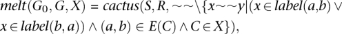where X is a set of chains in G and E(C) is, for the chain C, the set of block edges that it contains. This function therefore constructs an updated Cactus graph in which the alignments contained in X are absent. Figure 3, A and B, demonstrates this function. It is important to note how the removal of a chain can cause a local reorganization of the graph that can result in the formation of new longer chains.

Figure 3.

Melting and annealing examples. (A) An example showing the results of melt((G₀, G), X), where (G₀, G) is the Cactus graph in Figure 2C and X = {c}. (B) Like A, but with chain g also removed. (C,D) Examples of the effect of anneal((G₀, G), ∼∼), where (G₀, G) are the Cactus graphs in B and ∼∼ contains the alignments in chain c of the Cactus graph in Figure 2B added. (E) The MSLC solution for the Cactus graph in Figure 2C with large chain threshold α = 8. This is the result of the annealing function illustrated by C and D. The length of the longest chain in B increases by 2.

Adding further alignments to nets within G

As well as removing alignments, we can add them back into the graph, using the structure of G to filter which homologies to include. Let groups(G₀, G) return the set of groups in (G₀, G) and E(M) now be the set of adjacency edges in a group M. For cactus(S, R, ∼∼) = (G₀, G), let

where ∼∼′ is a new alignment relation and

where

This function only adds in alignments between positions in the same group, the rationale being that, given our confidence in the alignments of surrounding blocks, the positions in a net are more likely to be aligned together than to positions in other nets. Figure 3C–E demonstrates this function.

Tree coverage

As well as considering the minimum chain length as a parameter for accepting or rejecting a chain, we consider the amount of the species tree that the species in a chain cover.

A species tree T is an unrooted tree whose leaves are each assigned a unique species label and whose branches each have a positive real-number branch length. For a given species tree T, if we assume that each member of S is assigned a species label that also labels a leaf of T, then we can assign a tree coverage value to a chain. For a chain C, let S_C be the subset of S that has positions contained in one or more columns that label the edges of C. Let T_C be the induced subtree of T that includes only the leaves of T whose species label members of S_C. For a given T and S, treeCoverage(C, T) = branchLength(T_C)/branchLength(T), where branchLength is a function that returns the sum of the branch lengths in a tree.

Overview

Algorithm 1 outlines the CAF algorithm. The function length(C) returns the length of a chain C and chains(G) returns the set of chains in G. The algorithm takes, along with S, R, T, and ∼∼, two integer arrays, annealingArray and meltingArray, which represent values of α that are iterated over and a floating point minTreeCoverage value. It returns a Cactus graph for the inputs.

Algorithm 1. CAF (S, R, T, ∼∼, annealingArray, meltingArray, minTreeCoverage)

• Require ∀i, annealingArray[i] > 0

• Require ∀i, meltingArray[i] > 0

• Require ∀i < j, meltingArray[i] < meltingArray[j]

• Require 0 ≤ minTreeCoverage ≤ 1.0

  • (G₀, G) ← cactus (S, R, φ)

  • i ← 1

  • while i ≤ length (annealingArray) do

    • {Add alignments to groups}

    • (G₀, G) ← anneal(G₀, G, ∼∼)

    • {Progressively undo chains less than length annealingArray[i]}

    • j ← 1

    • while j ≤ length(meltingArray) do

      • if meltingArray[j] < annealingArray[i] then

        • (G₀, G) ← melt(G₀, G, {C|C ∈ chains(G) ∧

        • (length(C) < meltingArray[j]) ∨

        • treeCoverage(C, T) < minTreeCoverage)})

      • else

        • break

      • end if

      • j ← j + 1

    • end while

    • (G₀, G) ← melt(G₀, G, {C|C ∈ chains(G) ∧ (length(C) < annealingArray[i]) ∨

    • treeCoverage(C, T) < minTreeCoverage)})

    • i ← i + 1

  • end while

  • return (G₀, G)

The call to cactus sets up a Cactus graph containing only stubs and adjacency edges. The algorithm has two while loops; the top-level loop iterates over the integers in annealingArray. At the start of the outer loop, alignments are added to the graph; within the inner loop, chains of increasing length are progressively undone by iterating over progressively larger integers in the meltingArray. Consequently, at the end of an iteration of the top-level loop, G will contain no chains less than annealingArray[i] in length or with a tree coverage of less than minTreeCoverage. Therefore, by increasing the value of annealingArray[i] in the outer loop and in the inner loop melting increasingly larger chains, the algorithm attempts to iteratively extend larger chains while removing smaller and lower tree-covering chains that generally correspond to misalignments.

As a demonstration, if (G₀, G) = cactus(S, R, ∼∼) is the Cactus graph in Figure 2C, the MSLC solution shown in Figure 3C for α = 8 is found (for example) by CAF(S, R, T, ∼∼, [8], [2], 0).

The base-level alignment refinement algorithm

Let the size of a group be the sum of the lengths of the adjacency sequences that it contains. After applying the CAF algorithm, we find many of the groups' sizes in the resulting Cactus graph are typically below a few kilobases. We reason that once the size of a group is below a certain threshold, it makes sense to apply sensitive hidden Markov model (HMM)–based dynamic programming algorithms (Durbin et al. 1998) to align the adjacency sequences. Unfortunately, we cannot naively globally align the adjacency sequences in a group, as the group may involve rearrangements that prevent a partial ordering of the alignment; we have therefore developed an algorithm that we call the Base-level alignment refinement (BAR) algorithm.

Let M = (V(M), E(M)) be a (non-terminal) group in (G₀, G), where V(M) is a set of vertices in G₀ and E(M) is the set of adjacency edges that connect them. For a ∈ V(M), let S_a be the set of oriented adjacency sequences that label adjacency edges incident with a and let ∼∼_a be an alignment relation on the positions in S_a such that S_a defines a partial ordering between the columns (equivalence classes) defined by ∼∼_a. We call ∼∼_a an end alignment; it can be thought of as a poset global MSA for S_a. Let P(x_i∼∼y_j|x, y, θ), which we abbreviate henceforth to P(x_i∼∼y_j), be the posterior probability of x_i∼∼y_j given x, y, and a pairwise-HMM θ (Durbin et al. 1998). For each a ∈ V(M), the first step in the BAR algorithm is the construction of an end alignment ∼∼_a and imputation of a pairwise posterior probability for each member of ∼∼_a. These end alignments are constructed using code adapted from the Pecan global MSA program (Paten et al. 2009) (see Methods).

The union of the set of end alignments for a group will potentially contain a degree of spuriousness, because each adjacency sequence is contained in two independent end alignments constructed without regard to each other. The second step in the BAR algorithm is hence a simple strategy to “prune” the alignments.

Let x₁, x₂, …, x_n be an adjacency sequence labeling the adjacency edge (a, b), where a and b are in V(M). Let the cumulative alignment score for x_j and ∼∼_a be

Similarly, let

Let a cut point for x be an integer between 0 and n. For a cut point i, if i = 0, then the cut-point score equals score(−x₁, ∼∼_b), if i = n the cut-point score equals score(x_n, ∼∼_a), else i > 0 and i < n and the cut-point score equals score(x_i, ∼∼_a) + score(−x_i+1, ∼∼_b). A maximal cut point is one with a maximal cut-point score for the given adjacency sequence θ and pair of end alignments.

For an adjacency sequence x labeling adjacency edge (a, b) and a cut point j, a cut-point filtering is the removal of all x_k∼∼_ay from ∼∼_a, where k > j, and removal of all x_i∼∼_by from ∼∼_b, where i ≤ j. The pruning of the end alignments proceeds iteratively. We start with the initial set of end alignments. We pick an ordering (currently arbitrarily) of the adjacency sequences in the group, then for each adjacency sequence in turn, we find the optimal cut point and update the end alignments by performing a cut-point filtering for this optimal cut point. The end result of this procedure is a set of end alignments that do not overlap along any adjacency sequence. These “consistent” end alignments are then used to form a Cactus graph for the group, thus applying the BAR algorithm to each non-terminal group, we can construct a multilevel Cactus graph. As this computation is independent for each non-terminal group in the Cactus graph, the computation can be performed in parallel. An example of the BAR algorithm for one group is outlined in Figure 4.

Figure 4.

An illustration of the BAR algorithm. (A) A subgraph of an adjacency subgraph. The magenta and orange coloring of the blocks highlights the two chains; the outer A chain contains the inner B chain, which has been inverted in the red thread. (B) An example of the BAR algorithm. Box (1), four end alignments are constructed, one for each end in the net that contains ends of A and B. The alignments are oriented from their respective ends. These four alignments are inconsistent; if they were accepted as they are, they would together create many likely spurious alignments. Box (i), the blue adjacency sequence ACAT between a₁ and b₁, is chosen at random. A cut point is chosen (drawn as a red line) on an induced alignment, one containing only the columns with residues in the chosen adjacency sequence. The cut point must lie before the first, after the last, or between two residues in the adjacency sequence. The cumulative alignment score of aligned pairs to the adjacency sequence is shown below the two induced alignments, in both cases cumulated away from the respective block end. The cut point is chosen so that the cumulated score before the cut point in the induced alignment of a₁ plus the cumulated score after the cut point in the induced alignment of b₁ is maximal. Alignments to the adjacency sequence in the a₁ end alignment after the cut points are removed, and alignments to the adjacency sequence in the b₁ alignment before the cut points are removed. In this case, the cut point is after position 4, so all of the a₁ alignments are kept and all of the alignments to the adjacency sequence in the b₁ alignment are removed. Box (2), the result of removing the alignments discarded in (i). Boxes (ii–vi) and (3–7) show this process repeated for each of the remaining adjacency sequences in turn. The ordering of adjacency sequences in this process is random. (C) The resulting adjacency subgraph after the alignments in Box (7) of B are included. The adjacency sequences are now all empty, and there are three chains, the orange and magenta chains, which have been lengthened, and a single block cyan chain corresponding to an indel.

Alignment simulations

To test our methodology, we used the Evolver suite of genome evolution tools provided by Edgar, Asimenos, Batzoglou, and Sidow (http://www.drive5.com/evolver/), to produce two simulations of a 500-kb loci, one of a primate-like phylogenetic tree (human, chimp, gorilla, orangutan) and one of a mammal-like phylogenetic tree (human, dog, cow, mouse, rat) (see Methods).

Evolver models many rearrangement operations. Table 1 is a summary of the main operations that affect our simulations. Among others, Evolver models substitutions, insertions, deletions, tandem duplications, inversions, repetitive tranpositions (“M.E. Insert” in Table 1), segmental duplications (“Copy” in Table 1), and intra-chromosomal translocations (“Move” in Table 1). It also has a constraint model, which preferentially conserves genic and conserved non-coding elements, and numerous other biologically inspired features. These simulations represent the first time to our knowledge that Evolver has been used to assess alignment programs, and thus we purposefully chose limited simulations to allow us to manually assess the resulting output. Supplemental Figures S1 and S2 show dot plots of the evolved sequences. Figure 5 shows a dot plot of the simulated human and simulated mouse sequences for the Evolver mammals simulation; it is possible to observe insertions, inversions, translocations, and a segmental duplication.

Table 1.

An accounting of some of the simulated events that occurred during the burn-in, between the burn-in and the simulated human in the primate simulation, and between the burn-in and the simulated human in the mammal simulation, respectively

Figure 5.

A dot plot showing the Evolver mammals alignment of simMouse and simHuman. The true alignment is shown in blue, and overlaid in red is the predicted Cactus alignment. The density of different sequence annotations, as maintained by the Evolver model, are plotted on rows along the axes. (CDS) Coding sequence; (UTR) untranslated region; (NXE) non-exonic conserved regions; (NGE) non-genic conserved regions; (island) CpG islands; (tandem) repetitive elements. The gray box is expanded at the bottom of the figure for five different predicted alignments. Only the Cactus alignment correctly identifies the tandem duplication at the bottom left of the expanded region.

Evolver proceeds by evolving a set of sequences forward in time, while keeping track of the changes that separate ancestral sequences from their derived versions. Evolver therefore starts from a single root sequence. The root sequence and its annotations were taken from an actual human genomic loci (see Methods). We simulated forward evolution from the root genome for a total phylogenetic distance of 1.0 neutral substitutions per site in step sizes of 0.01, in order to generate the most recent common ancestor (MRCA) genome for subsequent simulations. This MRCA genome was then used as the input for both the Evolver primate and Evolver mammal simulation. We term this process a burn-in.

Producing a burn-in allowed us to check that the parameters for the simulations were close to stationarity, that is, the genome was not significantly shrinking or growing rapidly with simulation distance; and perhaps more importantly, it allowed us to establish a known evolutionary history over a lengthy time period for the entire genome. As such, for both simulations, we report two sets of precision/recall numbers, one including the evolutionary events during the burn-in and one excluding them.

We do this for three reasons. Firstly, the burn-in inclusive homology relation contains many pairs that we have no reasonable hope of correctly aligning; it is thus unduly severe to use only this set to calculate recall. Secondly, and conversely, the burn-in exclusive homology relation excludes many pairs that we should reasonably judge as being homologous; thus, it is unduly harsh to use only this set to calculate precision. Thirdly, it is interesting to contrast our ability to align events that occurred before the MRCA to those that occurred after the MRCA. However, to avoid overcomplicating matters, we sought a single measure that avoids the first two issues to measure overall accuracy. To do this, we use a standard F_β score (Rijsbergen 1979), where β is used to adjust the weight placed on precision versus recall, in which we use the burn-in inclusive homology relation to calculate recall and the burn-in exclusive homology relation to calculate precision.

One important issue with Evolver is that it does not consider independently inserted copies of the same transposon as homologous. This is understandable, given that there may be many thousands or hundreds of thousands of copies of related elements in a single genome; and thus it is both unreasonable and impractical to consider instances of these elements to be homologous. However, this behavior is also problematic: firstly, because such elements have evolved in vivo by a process of duplicative transposition that, in the case of segmental duplication, we do consider to be a generator of homology (and that Evolver does separately model); secondly, and more practically, because multiple copies of a transposon introduced in a short period of time appear homologous, but yet are not considered homologous by Evolver. Thus in these simulations, the homology relation can be considered to be conservative because it excludes certain pairs that might otherwise reasonably be considered to be homologous.

In addition to testing with these novel simulations, we used a set of previously published simulations generated by Blanchette et al. (2004b). Their simulations attempt to model the neutral region evolution of nine extant mammalian species: human, chimp, baboon, mouse, rat, dog, cat, cow, and pig. The simulations comprise 50 50K alignments. The mutational operators considered included substitutions; CpG effects; insertions, including the action of transposed repetitive elements; and finally, deletions. Importantly, the Blanchette simulations do not model any nonlinear rearrangements that break the partial ordering of the sequences with respect to one another; thus, they are appropriate for assessing programs that generate global MSAs as well as partially exercising those that can generate more general forms of MSA. The root sequences for these simulations were generated from a Markov process, and thus are assumed to contain no self-homology; hence, no burn-in is necessary for these simulations. These simulations also contain repeat elements, which are not treated as homologous and which therefore create the same issues as discussed above for the Evolver simulations.

Testing CAF

To test the CAF algorithm, we experiment with two values for each of the melting and annealing arrays, giving four possible combinations. Either the annealingArray contains a single value, which we call simple annealing, or a monotonically increasing array of values, which we call progressive annealing. Similarly, either the meltingArray is empty, which we call simple melting, or it contains a monotonically increasing array of values, which we call progressive melting. We experiment with different maximum values in these arrays, which can be thought of as the value of α, in all cases using a range of powers of 2, from 4 to a maximum of 8192. For a default tree coverage of 0.8, Figure 6 shows the effects of these four combinations for the three different simulations for different maximum values of α.

Figure 6.

The effects of altering the minimum chain length α on the alignment predicted by the CAF algorithm. (A–C) Using the Evolver mammals data set. (D–F) Using the Evolver primates data set. (G–I) Using the Blanchette data set. (A,D,G) Precision-recall plots. The variable α is altered in powers of 2 from 4 to 8192. In general, increasing α increases precision and decreases recall. Four strategies are shown, for the four combinations involving simple melting/progressive melting and simple annealing/progressive annealing. (B,E,H) The F_0.25 score (weighting precision fourfold over recall) as a function of α, for the four CAF strategies (colors consistent with [A,D,G]). (C,F,I) The computation time (using a single contemporary 0 × 86 processor) as a function of α.

Precision-recall (Fig. 6A,D,G) plots show the trade-off between these measures as a function of α. As expected, larger values of α produce higher precision but lower recall. To choose a default value for α, we calculate the F_0.25 score (Fig. 6B,E,H), which weights precision four times over recall; as the CAF algorithm is used to choose the alignment map on which the BAR algorithm will be run, we weight precision more highly than recall at this stage. We also plot (Fig. 6C,F,I) the computation time for running CAF in these evaluations.

Let the combined simple melting and simple annealing strategy be called the naive strategy. We find that compared to the naive strategy, the strategy involving progressive melting and simple annealing increases precision by 4.1% on average, increases recall 16.4% on average, and increases the F_0.25 score 14.9% on average, where the average is over all simulations and all tested values of α. We find using the same form of comparison that the strategy involving progressive annealing and simple melting increases precision 5.8% on average, increases recall 15.9% on average, and increases the F_0.25 score 17.7% on average, compared to a naive strategy. Combining both progressive melting and progressive annealing does not significantly change precision or recall on average over using progressive annealing and simple annealing alone. Many of these differences come from larger values of α; using an α value up to 256, we find that the progressive melting/annealing strategy is 2.9% on average better in precision and does not significantly alter recall, resulting in an average 6.8% increase in the F_0.25 score.

The progressive annealing strategy adds most significantly to computation time, while the progressive melting strategy adds only marginally versus the naive strategy. This is largely because the former currently requires linearly traversing the set of input alignments, which is relatively slow, while the latter requires only a recalculation of the Cactus graph, which is linear time in the size of the elements in the adjacency graph and relatively quick.

The differences in the F_0.25 score for each simulation are quite small across a wide range of values. The value of α that gives the highest F_0.25 score for the Evolver mammals and the Blanchette simulation is 32 for the non-naive strategies. For the Evolver primates simulation, the F_0.25 score is close across a range of values, but peaks at α = 1024. This difference partly reflects the much lower values of recall that are achieved in the mammal and Blanchette simulations by the CAF algorithm, and partly seems to relate to the alignment of transposons, which we address in the next section.

Testing BAR

To test the combined CAF and BAR algorithms, we perform the same analysis as described for the CAF algorithm alone; the results are shown in Figure 7 and laid out as in Figure 6, the only difference being that we now plot the F₁ measure in Figure 7B,E,H, as we are now equally interested in precision and recall.

Figure 7.

The effects of altering the minimum chain length α on the combined results of the CAF and BAR algorithms (the implementation is collectively called Cactus). The format of the figure is the same as in Figure 6, except F₁ scores are shown in plots B, E, and H.

The relationship between precision and recall follows the same simple trade-off relationship in the Evolver mammals simulation. The Evolver primates and Blanchette simulations, however, show a more complex relationship. In the former case, there is an apparent step in the curve that suddenly increases precision at α = 1024, after which the curve reaches an asymptotic limit. In the case of the Blanchette simulations, the relationship between precision and recall is not a trade-off; rather, for a range of α between 4 and 2048, the precision and recall both increase. For values greater than α = 2048, the result then collapses, as no chains of this length can be reliably found within the simulations, and thus the algorithm generally returns a trivial alignment containing no aligned pairs.

Both the Evolver primate and Blanchette results circumstantially appear influenced by the two simulators' treatment of repetitive transposition, which we discussed above. To attempt to discern this effect in the Evolver simulations, we reran them with repetitive transposition turned off. Figure 8 shows the results in terms of precision and recall for the Evolver primates simulation (see Supplemental Fig. S3 for the equivalent figure for the Evolver mammals simulation). We note that the steplike change in precision that occurs at α = 1024 is gone in the no-transposons simulation; rather, the curve shows a smooth relationship between precision and recall, and precision as a function of α reaches its asymptotic limit earlier, at ∼α = 64. We conclude therefore that, at least in the Evolver simulations, the issue of repetitive transposition significantly affects the result.

Figure 8.

Comparing the effect of removing the repetitive transposition operation on two independent runs of the Evolver primates simulation, one including and one without the operation. (A) A precision-recall plot of the predicted Cactus alignments showing the effect of altering α in powers of 2 from 4 to 8192. (B) The precision as a function of α. Note particularly the step-up in precision between α = 512 and α = 1024 for the simulation including repetitive transposition, whose alignment is not considered homologous by Evolver.

Questions remain as to how much the operation of repetitive transposition disrupts the correct alignment of homologies recognized by Evolver, and how much Evolver's decision to not recognize homologies created by independently inserted repetitive transpositions artificially biases the result against shorter values of α. After manual analysis of both the Evolver primate and Blanchette simulations, we strongly suspect that the latter explanation largely accounts for this effect, although it is probable that the former effect is not negligible. In future work, we therefore plan to better address this homology problem by formulating methods to identify repetitive homologies and classify them into those that cannot reasonably be justified, and those that can. However, for the remainder of this analysis, we test two versions of Cactus that are identical with the exception that in one α = 64 and in the other α = 1024. We call the former simply Cactus, and it is the default mode of the program; the latter we call Cactus No Transposons [Cactus (N.T.) in the tables]. When we compare Cactus to existing programs (see below), we show results for both.

We find that the progressive annealing and melting strategy has 15.4% higher recall on average, 14.1% higher precision on average, and 14.7% higher F₁ score than a naive strategy, where the average is over all simulations and all values of α. However, as with the CAF algorithm alone, much of this effect comes from higher values of α, looking again at values of α from 4 to 256, we find a 0.9% increase in precision and 0.8% decrease in recall, leading to a marginal 0.24% increase in overall F₁ score. For small values of α, we conclude that the BAR algorithm is largely able to compensate for differences between the different strategies in terms of precision and recall. However, we find that the overall computation time of the BAR and CAF algorithms over all simulations is, on average, lowest when progressive annealing and melting is enabled. For this reason, and because they are robust to increases in α, we therefore select them as defaults.

For all of the above comparisons of the two algorithms, we used a minimum tree coverage of 0.8. Figure 9 shows the effect of adjusting the minimum tree coverage on the combined results of the CAF and BAR algorithms. We find that for values of α <32, a minimum tree coverage of 1 is best. This is likely because it is advantageous to have complete tree coverage when choosing to accept very short chains. For values of α >16, we find that a minimum tree coverage of 0.8 gives the highest F₁ scores.

Figure 9.

The effects of adjusting tree coverage. (A) A precision-recall plot of the predicted Cactus alignments showing the effect of altering α in powers of 2 from 4 to 8192. Four curves are plotted, showing changes in minimum tree coverage from 0 to 1.0 (see key in A). (B) The F₁ score as a function of α for the four different minimum tree coverages (colors consistent with A). (C) As in B, but showing time.

The BAR algorithm uses the posterior probabilities of aligned pairs to choose how to trim sets of end alignments and make them consistent. We can also use a threshold that we call γ on the sum of posterior probabilities in a column to choose to accept or reject the pairs it contains (see Methods), in a similar fashion to that described in Schwartz and Pachter (2007). Figure 10 shows the effects of adjusting γ on the resulting alignments. By adjusting γ we can achieve a smooth trade-off between precision and recall in the simulations involving pan-mammalian comparisons. In the Evolver primates simulations, very few pairs are uncertain, and hence the parameter has little effect.

Figure 10.

The effect of adjusting γ. (A) A precision-recall plot of the predicted Cactus alignments showing the effect of altering γ, for the three different alignment simulations. (B) The F₁ score as a function of γ for the three different simulations; shapes consistent with A.

Comparisons to existing programs

Finding freely available programs to compare with was surprisingly difficult; we found relatively few contemporaries that were easily capable of aligning all of these simulations. We tested Pecan (Paten et al. 2009), FSA (Bradley et al. 2009), Multiz (Miller et al. 2007), TBA (Blanchette et al. 2004b), and progressiveMauve (Darling et al. 2010). Pecan is our program for large-scale global MSA generation and has previously been shown to perform well in the Blanchette simulation (Paten et al. 2008). FSA is another large-scale global MSA program that optimizes a slightly modified AMAP score (Schwartz and Pachter 2007). In our hands, we could not make it scale to align the Evolver simulations in reasonable time or memory, but expect it to perform similarly to Pecan in these benchmarks. Multiz is used by the UCSC browser (Fujita et al. 2011) to create whole-genome reference-based MSAs; as such, it does handle nonlinear rearrangements, but it does not allow for duplications and is likely to perform best for the chosen reference sequence. TBA builds on Multiz and uses more extensive dynamic programming to make the alignment symmetrical (non-reference-based). We also tested a version of TBA used during the ENCODE pilot project (Margulies et al. 2007), which allows for duplication of non-reference bases. Progressive-Mauve is a new and more sensitive version of the Mauve genome alignment program (Darling et al. 2004) that handles nonlinear rearrangements although not duplications.

The global MSA programs Mavid (Bray and Pachter 2004) and Mlagan (Brudno et al. 2003a) were excluded from comparison because they had previously performed more poorly than those we tested in the Blanchette benchmark (Blanchette et al. 2004b; Paten et al. 2008) and have not been updated. The shuffle-Lagan program (Brudno et al. 2003b) does handle rearrangements, but is pairwise only, does not handle duplications, and could not be made to run stably in our hands. The synteny mapping programs Enredo (Paten et al. 2008) and Mercator (Dewey 2007) are not currently suitable for these benchmarks, as they require sets of predetermined “anchor” alignments, such as those of exons, which, due to the relatively small size of the simulations, are both few and not readily computable by an existing method. All the tested programs were run with their default parameters and using the latest versions available, with a few exceptions (see Methods).

Tables 2, 3, and 4 show the results for the Evolver mammals, Evolver primates, and Blanchette simulations, respectively. We break the results down into a number of categories. For the Evolver simulations, we give categories both excluding and including the burn-in period. For all tables, we show the results over all (“All” columns) pairs, and results for just pairs involving human sequences (“Human” columns), which we used as a reference sequence for those programs that need a reference (Multiz and ENCODE TBA). We also look at pairs, including (“All” rows), excluding (“No repeats” rows) and only containing pairs (“Repeats” rows) where one or both sequence positions has been deemed repetitive by the repeat masking. Finally, we attempt to discount local misalignment using the near category (“Near” rows). For any homologous pair x_i∼y_j, if x_i+k∼∼y_j or x_i∼∼y_j+k for −n ≤ k ≤ n, where n is a mis-alignment parameter (in all these comparisons n = 5), we consider x_i∼y_j to be contained in ∼∼ when calculating absence and spuriousness. Symmetrically, for the aligned pair x_i∼∼y_j pair if x_i+k∼y_j or x_i∼y_j+k for −n ≤ k ≤ n, we consider x_i∼∼y_j to be contained in ∼ when calculating absence and spuriousness. Thus, small misalignments are acceptable in the near category, while larger misalignments are penalized, and thus the Near row numbers are always equal or improvements on the All row numbers.

Table 2.

Comparisons using the Evolver mammals data set

Table 3.

Comparisons using the Evolver primates data set

Table 4.

Comparisons using the Blanchette data set

In the Evolver mammals simulation, the default Cactus program substantially outperforms all other programs in terms of recall and F₁ score in all categories, and, in fact, in every possible pairwise comparison of the constituent species (see Supplemental Tables S1–S5). In terms of precision, the Cactus (N.T.) program has slightly higher overall precision, although by only ∼0.3%. The other programs perform largely as expected. Pecan has good precision, but its inability to handle nonlinear rearrangements means that it cannot align some sequences and so correspondingly has poor recall. TBA and Multiz are quite close in overall precision and recall, although Multiz performs significantly better in human reference terms and significantly worse in non-human reference terms (see the Supplemental Material). Only progressive-Mauve performs substantially more poorly than might be expected; after discussion with the author, the problem appears to be related to a failure in the automatic detection of a “weight” parameter; therefore, with parameter adjustment, this result might be improved.

In the Evolver primates simulation, the difference between the programs is smaller, as might be expected, given the relative simplicity of the majority of this alignment problem. We find that our Cactus (N.T) program has the highest F₁ score, but that TBA and the Cactus default programs are very close behind. The previously noted issues with homology produced from repetitive transposition arise in the benchmark, meaning that the precision numbers should be considered a conservative measure that may discount some homologies that may be considered reasonable. We note that Multiz achieves high human-reference recall, although at an apparently high cost in terms of precision.

In the Blanchette simulation, our Pecan program was previously the best performing in terms of recall and F₁ score. We find that Cactus (N.T.) outperforms it in terms of precision and F₁ score, although the difference between Pecan and Cactus is relatively small compared to the other programs considered, which generally have much poorer recall. We note that in this benchmark and in the Evolver primates, benchmark progressive-Mauve appears to perform somewhat better. The FSA program, which we could run on this benchmark, produces good precision, but its recall is relatively poor.

Primate gene alignments

We have analyzed our methods using simulation. We can also do empirical analysis of the alignments of actual biological sequences. There are many different possible approaches (see (Margulies et al. 2007 and Paten et al. 2008 for interesting biological metrics), in this study, we examined the conservation of genes and exons and compared and contrasted our results with the human reference Multiz alignments (Miller et al. 2007) hosted by the UCSC browser (Fujita et al. 2011), which are probably the most cited set of existing genomic alignments.

We chose the first 10 ENCODE pilot project regions (ENm001–ENm010) (Margulies et al. 2007) and constructed alignments for a set of primates (human, chimp, orangutan, and rhesus) (see Methods). These alignments were selected because we thought that they gave a reasonably sized set of genes and corresponding alignments whose evolutionary distance made manual analysis of all the results possible.

We collected all human RefSeq mature mRNA transcripts (NM* accession) that are located within the 10 selected regions, and looked for homologs of their CDSs (coding sequences) in other species using the alignments (see Methods). For each gene that had multiple transcripts, we only selected the transcript with the longest CDS to prevent repeat penalization. We will refer to these human CDSs as the reference CDSs.

In each non-human species, we call a sequence that aligns to a human exon a conserved homolog if (1) it has a total insertion and deletion size (total indel size) that is a multiple of 3, and (2) neither the insertion nor deletion size exceeds 10% of the reference exon length; else we call it a non-conserved homolog. A non-conserved homolog that contains more than 10 contiguous wildcard Ns (generally representing a scaffold breakpoint) is deemed to have missing data, describing the state in which there is not enough information to deem if the sequence could have been correctly aligned.

An exon is defined as conserved if there is at least one conserved homolog in every species; else it is non-conserved. An exon that is non-conserved has missing data if at least one homolog sequence in the alignment contains missing data.

In each species a sequence that aligns to the exons of a human gene is similarly called a conserved homolog of the gene if it contains a conserved homolog of each exon in the same order and orientation as the reference gene; else it is called a non-conserved homolog of the gene. For genes we say that a non-conserved homolog of a gene has missing data if it contains any non-conserved exon homologs.

Consistent with the definition of exon conservation across species, a gene is defined as conserved if there exists at least one conserved homolog in every species; else it is non-conserved. As with exons, a gene that is non-conserved has missing data in the alignment if at least one homolog sequence aligned to a reference exon contains missing data.

There were a total of 1776 exons in 232 genes. Ninety-four genes (40.52%) and 100 exons (5.63%) were removed from the comparison because (1) they were not conserved by both Multiz and Cactus; and (2) the alignments were found to contain missing data (as described above). Many of those classified as having missing data were missing substantial portions of sequence, typically involving entire exons.

Table 5 shows a comparison of cross-species conservation between Cactus and Multiz. We find that there is a high degree of concordance between the two methods at both the exon and gene level, but with Cactus predicting a smaller number of non-conserved genes and exons than Multiz. When a gene was conserved by one program's alignment but not conserved by the other program's alignment, it was always due to the non-conservation of an exon.

Table 5.

Comparisons of genic and exonic cross-species conservation between Cactus and Multiz using primate alignments

Where Cactus predicts a conserved exon but Multiz does not (75 cases) (see Supplemental Table S9), we find 40 cases in which Multiz fails to align a homologous sequence in one or more species (for an example, see Supplemental Fig. S5). We find 29 cases in which Multiz aligns a homologous sequence in every species, but, because it must choose just one such sequence per species, it picks a homolog in at least one species that does not conserve the exon (for examples, see Supplemental Figs. S6, S7). In the remaining six cases, the Multiz alignments contain a large indel in one or more species' homologous sequences. Interestingly, upon further investigation, each such indel apparently arose by a tandem duplication, a process that can apparently confuse Multiz into aligning the prefix of the 5′ copy and the suffix of the 3′ copy to the single human copy, leaving the remainder of the duplication as an indel (Supplemental Fig. S8 shows an example). In each of these tandem duplication cases, Cactus properly aligns both copies together.

Where Multiz predicts a conserved exon but Cactus does not (11 cases) (see Supplemental Table S9), we find that Cactus has failed to align a homolog in 10 cases (for an example, see Supplemental Fig. S4) and aligned a homolog that was not conserved in the other case.

While the Evolver simulations were too small to contain significant amounts of duplication, these 10 loci allow us to observe the performance of our program when dealing with duplications. As mentioned, while the Multiz alignments can give no indication of duplications, the Cactus alignments predict that 346 (19.48%) exons, 542 of 1544 introns (35.1%), 161 genes including exons and introns (69.4%), and 112 genes including only exons contain duplication. Many of these duplications are between paralogous members of gene families, but we also find cases that correspond to short intra-gene tandem and local segmental duplications (as in Supplemental Fig. S8).

Discussion

We have described two novel algorithms for genome alignment whose combination produces alignments that allow for nonlinear rearrangements and duplications and yet achieve good levels of precision and recall, overall outperforming all their existing peers. The implementation is freely available (see Methods) and can be used to align substantial genomic loci or megabase-scale genomes. We believe therefore that the program will prove useful for many comparative genomics efforts. However, we are also aware of the need to scale it to handle clades of entire mammalian size genomes. Given the recursive, nested nature of the Cactus graph structure that we build, we believe that this will be possible and, indeed, efficient. It is our intention that the Cactus program will shortly provide complete genomic alignments, and that these will be available within the UCSC Genome Browser.

We have described the MSLC problem and the CAF algorithm for finding (non-optimal) solutions. The MSLC problem has similarities with and was somewhat inspired by the Maximum Weight Subgraph with Large Girth (MSLG) problem for A-Bruijn graphs proposed by Pevzner et al. (2004). In that problem, the investigators aim to rid the A-Bruijn graph, which has similarities to an adjacency graph, but does not represent the difference between x∼∼y (or equivalently −x∼∼−y) and x∼∼−y (or equivalently −x∼∼y) (for a discussion of this topic, see Medvedev and Brudno 2009), of cycles with a girth (number of edges) less than a threshold, these low girth cycles typically resulting from spurious alignments, very short tandem repeats, and indels. The result of solving the MSLG problem is a subgraph that does not properly represent all the input sequences, many adjacencies and subsequences having been removed. In the MSLC problem, the resulting Cactus graph does still properly represent all the input sequences, the difference between the input and output being in the represented set of alignments—this therefore avoids any problem of threading the input sequences back through the resulting graph.

We have also described the BAR algorithm, which attempts to make consistent a set of overlapping global poset MSAs. We have found that the combination of the CAF and BAR algorithms provides significant benefit over applying the CAF algorithm alone, particularly in terms of improving recall. In both algorithms we have used the structure of the Cactus graph, in the CAF algorithm to filter the alignments, and in the BAR algorithm to decompose the problem into a set of independently alignable nets. Given that the cumulative run time of the BAR algorithm far exceeds that of the CAF algorithm, the ability to apply the BAR algorithm in parallel provides essential performance.

We have created challenging Evolver genome simulations and comprehensively benchmarked our program against its peers. Additionally, we have tested our program against an established benchmark, the Blanchette et al. simulations (Blanchette et al. 2004a). It is beyond the scope of this study to establish in general how realistic these simulations are. Clearly, both have limitations to their complexity; for example, neither models gene conversion events or transcription factor binding site evolution, each of which might be needed for accurate simulation of certain genomic loci. However, we note that both simulations, covering similar groups of species, show reasonable concordance in their individual pairwise species predictions of recall and precision for our Cactus alignments. This is despite the fact that the Evolver simulations both include all the operations modeled by the Blanchette simulations, and indeed those modeled by similar methods such as Varadarajan et al. (2008), and add numerous extra mutational operators. This supports the notion that certain classes of highly prevalent mutation, e.g., substitutions and indels, dominate other, rarer operations, such as inversions and translocations, when assessing overall recall and precision.

We have also tested our genome MSAs using an analysis of how well our method aligns known genes within large genomic loci. Our analysis of primate gene alignments suggests that there is rampant duplication present in the genic sequences. Some of this may correspond to assembly artifacts, but it is probable that many cases reflect real biology.

The Supplemental Material for this study can be found at http://hgwdev.cse.ucsc.edu/^∼benedict/code/Cactus_files/cactusAlignmentSupplement.zip.

Methods

Cactus implementation

We have implemented the CAF and BAR algorithms in a new program called Cactus. The basic inputs to the program are a set of “genomes,” a genome being simply one or more multiple fasta files, and a tree, which may have nodes of arbitrary degree (not just binary), describing the relationships between the input genomes that are assigned to its leaves. Additionally, a configuration file describing parameters to the various algorithms can be provided as input; otherwise, the default settings are used. The output of Cactus is a database. Cactus works with a variety of database engines, including the SQL databases MySQL (http://www.mysql.com/) and PostgreSQL (http://www.postgresql.org/), the embedded interface to the NoSQL database Tokyo Cabinet (http://fallabs.com/tokyocabinet/), and the remote interface to the NoSQL database Kyoto Cabinet (http://fallabs.com/kyotocabinet/), which currently offers the highest performance on computational clusters. The output database can be accessed via a C API, but a number of command-line utility scripts are available to convert the alignment into a standard format, such as MAF format (http://genome.ucsc.edu/FAQ/FAQformat.html).

The source code, written in C and Python, is open source and freely available from https://github.com/benedictpaten/cactus/tree/genome_research_alignment_paper, with the exception that certain third-party source code that is redistributed, with permission, within the source tree has more restrictive license requirements (see https://github.com/benedictpaten/cactus/blob/master/externalTools/LICENSE.txt). Among other dependencies, Cactus requires our open source cluster management software Jobtree (https://github.com/benedictpaten/jobTree) and can be made to work on a single machine, with multiple processors or on a computer farm of separate machines. The source code includes a manual describing how to run the software to generate a genome MSA of the type described here (see https://github.com/benedictpaten/cactus/raw/master/doc/README.pdf).

CAF parameters

To compute the alignment relation for the CAF algorithm, we use Lastz (http://www.bx.psu.edu/miller_lab/dist/README.lastz-1.01.50/README.lastz-1.01.50.html), which is also a requirement for running Cactus. In computing the initial alignment relation, we prefer recall over precision, as the CAF algorithm provides an effective filter. Lastz is hence run with its default parameters, except that we use the parameter “--hspthresh=1800,” to lower the threshold for accepting high-scoring segment pairs (HSPs) to the gapped extension stage.

End alignments

To construct the alignment for adjacency sequences incident with an end, we use code adapted and ported to C from Pecan's Java code. By default, we use the same five state pair-HMMs described in Paten et al. (2009), which features two pairs of affine gap states, to compute pairwise posterior probabilities. For a set of sequences S being aligned, let be the number of unique pairwise comparisons. If n < 10 * |S|, we compute posterior probabilities for every pair of sequences; else we compute a random sample of 10 * |S| pairwise alignments and use this as the alignment relation ∼∼. This logic therefore prevents the number of pairwise alignments being computed from scaling quadratically with the number of sequences while using all pairwise comparisons when practical.

To construct a poset MSA from ∼∼ and S, we use the same greedy “sequencing annealing” algorithm described in Schwartz and Pachter (2007), creating our own C implementation of an online topological order constraint algorithm described in the supplement of Paten et al. (2009). The algorithm proceeds by greedily constructing a series of alignments ø, ∼∼₁, ∼∼₂, …, ∼∼_n. For ∼∼_i, let C_i be the set of columns (equivalence classes) defined by ∼∼_i. The next alignment relation ∼∼_i+1 = ∼∼_i ∪ X × Y, where X and Y are two columns in C_i such that the weight

is maximal over all valid pairs of columns in C_i and where poset(∼∼) is an indicator function that returns 1 if and only if the ordering relation defined by the sequences in S on the columns of ∼∼ is a partial ordering. The sequence of alignments terminates when no such pair of columns exists. It is easy to verify that the sequence of merges has monotonically decreasing weight.

In a nutshell, the alignment therefore constructs a poset MSA by greedily considering the members of ∼∼ in an order that relates to their posterior probabilities. The central difference between our implementation and that of Schwartz and Pachter (2007) is that we do not consider gap probabilities when merging columns. Instead, we use a γ parameter, a real number in the interval [0, 1], and return the last alignment in the sequence that was produced by a merge of two columns X, Y for which

Evolver alignment simulations

The phylogenies and branch distances were based on the Human/hg19/GRCh37 46-way multiple alignment (Fujita et al. 2011). The simulated primate tree was “((simGorilla:0.008825,(simHuman:0.0067,simChimp:0.006667):0.00225):0.00968, simOrang:0.018318).” The simulated mammal tree used was “((simCow:0.18908,simDog:0.16303):0.032898,(simHuman:0.144018,(simMouse:0.084509, simRat:0.091589):0.271974):0.020593).”

We generated a “root” genome by pulling the FASTA sequence for Hg18 chromosome 6 positions 132,218,540–132,718,539 from the UCSC Table Browser, along with the corresponding annotations from UCSC Genes, UCSC Old Genes, CpG Islands, Ensemble Genes, and MGC Genes (Fujita et al. 2011). We created a simple Makefile to automate in-file set generation, following details available from the Evolver manual.

We used a parameter set tuned for a mammalian ancestral genome consisting of 23 chromosomes provided by Arend Sidow (pers. comm.). We scaled the parameters related to inter-chromosomal evolution (e.g., inter-chromosomal movement rates [InterChrMoveRates] and inter-chromosomal copy rates [InterChrCopyRates]), by the ratio of the size of our simulations' root genome (500,000 bp) to Hg18 (2,881,421,696 bp) for a conversion factor of 1.7353 × 10⁻⁴.

We scaled parameters related to intra-chromosomal evolution (chromosomal fusion rate [ChrFuseRate], chromosomal fission rate [ChrSplitRate], reciprocal translocation rate [RecipTranslocRate], and non-reciprocal translocation rate [NonRecipTranslocRate]), by the ratio of the number of chromosomes in our simulations' root genome to the approximate number of chromosomes in Hg18.

We used a mobile element library provided by Arend Sidow (pers. comm.) as input to the burn-in simulation and allowed each simulated genome to inherit the library from its parent genome and to evolve the library for a short period before drawing mobile elements in the standard method outlined in the Evolver manual. Due to the short size of the region being evolved (500 kb) and the fact that it originally contained only one gene, we turned off the retroposed pseudogene feature in Evolver's parameter file.

Following simulation, FASTA sequences were extracted for leaf genomes and repeat masked using RepeatMasker. For the primate simulation, we presented RepeatMasker with the mobile element library of the MRCA genome, reasoning that this library was a reasonable length from all the extant genomes and thus avoiding making an unrealistically good repeat masking. For the mammal simulation, we presented RepeatMasker with a library made up of the mobile element libraries of both the MRCA and of the simulated human–mouse–rat ancestor.

The simulations are available as raw sequences and MAF alignments as part of the Supplemental Material.

External program parameters

All the tested programs were run with their default parameters and using the latest versions available with the following exceptions. For FSA we used the “--exonerate --softmasked” flags, which are advised by the authors for longer, soft-masked sequences. For Multiz, after consultation with the authors, we used their “roast” script with human specified as the reference. For the ENCODE version of TBA we added “+ E = human” flags to specify that human was the reference sequence. For Progressive-Mauve we used the latest nightly snapshot (dated 2011-01-25), after consultation with the authors, to work around known bugs that affect accuracy in the stable release.

Primate gene alignments

We chose the first 10 ENCODE pilot project regions for our empirical analysis. The sequence coordinates were obtained from the UCSC hg18 human assembly browser database (see Supplemental Table S11). The Multiz alignments for each region were extracted from the Multiz 44-way alignments obtained from the UCSC hg18 browser database.

To generate the Cactus alignments, we used the region coordinates obtained above to obtain the human DNA sequences. For the other species we used the Multiz 44-way alignments as pointers to locate where on these species' genome each ENCODE region is mapped. We included all the sequence fragments of the species that were aligned to each ENCODE region. Fragments that are within 1 Mb of each other were put together in one bin. We then used the minimum and maximum coordinates (all coordinates were converted to be on the positive strand) of the resulting bins to pull out the corresponding raw sequences from the appropriate assembly (see Supplemental Table S11). Cactus was run with default parameters. The tree and branch distances for the primates were extracted from the UCSC 44-way tree: “(((hg18:0.003731,panTro2:0.005501):0.02301,ponAbe2:0.02):0.02,rheMac2:0.031571).”

The Cactus alignments generated are available as MAF alignments as part of the Supplemental Material.

References

- Blanchette M, Green ED, Miller W, Haussler D 2004a. Reconstructing large regions of an ancestral mammalian genome in silico. Genome Res 14: 2412–2423 [DOI] [PMC free article] [PubMed] [Google Scholar]
- Blanchette M, Kent WJ, Riemer C, Elnitski L, Smit AFA, Roskin KM, Baertsch R, Rosenbloom K, Clawson H, Green ED, et al. 2004b. Aligning multiple genomic sequences with the threaded blockset aligner. Genome Res 14: 708–715 [DOI] [PMC free article] [PubMed] [Google Scholar]
- Bradley RK, Roberts A, Smoot M, Juvekar S, Do J, Dewey C, Holmes I, Pachter L 2009. Fast statistical alignment. PLoS Comput Biol 5: e1000392 doi: 10.1371/journal.pcbi.1000392 [DOI] [PMC free article] [PubMed] [Google Scholar]
- Bray N, Pachter L 2004. Mavid: Constrained ancestral alignment of multiple sequences. Genome Res 14: 693–699 [DOI] [PMC free article] [PubMed] [Google Scholar]
- Brudno M, Do CB, Cooper GM, Kim MF, Davydov E, Program NCS, Green ED, Sidow A, Batzoglou S 2003a. Lagan and multi-lagan: Efficient tools for large-scale multiple alignment of genomic DNA. Genome Res 13: 721–731 [DOI] [PMC free article] [PubMed] [Google Scholar]
- Brudno M, Malde S, Poliakov A, Do CB, Couronne O, Dubchak I, Batzoglou S 2003b. Glocal alignment: finding rearrangements during alignment. Bioinformatics (Suppl 1) 19: i54–i62 [DOI] [PubMed] [Google Scholar]
- Darling ACE, Mau B, Blattner FR, Perna NT 2004. Mauve: Multiple alignment of conserved genomic sequence with rearrangements. Genome Res 14: 1394–1403 [DOI] [PMC free article] [PubMed] [Google Scholar]
- Darling AE, Mau B, Perna NT 2010. progressiveMauve: Multiple genome alignment with gene gain, loss and rearrangement. PLoS ONE 5: e11147 doi: 10.1371/journal.pone.0011147 [DOI] [PMC free article] [PubMed] [Google Scholar]
- de Bruijn NG 1946. A combinatorial problem. Volkskunde 1: 758–764 [Google Scholar]
- Dewey CN 2007. Aligning multiple whole genomes with mercator and mavid. Methods Mol Biol 395: 221–236 [DOI] [PubMed] [Google Scholar]
- Dubchak I, Poliakov A, Kislyuk A, Brudno M 2009. Multiple whole-genome alignments without a reference organism. Genome Res 19: 682–689 [DOI] [PMC free article] [PubMed] [Google Scholar]
- Durbin R, Eddy S, Krogh A, Mitchison G 1998. Biological sequence analysis. Cambridge University Press, Cambridge, UK [Google Scholar]
- Feng DF, Doolittle RF 1987. Progressive sequence alignment as a prerequisite to correct phylogenetic trees. J Mol Evol 25: 351–360 [DOI] [PubMed] [Google Scholar]
- Fujita PA, Rhead B, Zweig AS, Hinrichs AS, Karolchik D, Cline MS, Goldman M, Barber GP, Clawson H, Coelho A, et al. 2011. The UCSC Genome Browser database: update 2011. Nucleic Acids Res 39: D876–D882 [DOI] [PMC free article] [PubMed] [Google Scholar]
- Harary F, Uhlenbeck GE 1953. On the number of husimi trees: I. Proc Natl Acad Sci 39: 315–322 [DOI] [PMC free article] [PubMed] [Google Scholar]
- Higgins DG, Bleasby AJ, Fuchs R 1992. CLUSTAL V: improved software for multiple sequence alignment. Comput Appl Biosci 8: 189–191 [DOI] [PubMed] [Google Scholar]
- Lee C, Grasso C, Sharlow MF 2002. Multiple sequence alignment using partial order graphs. Bioinformatics 18: 452–464 [DOI] [PubMed] [Google Scholar]
- Margulies EH, Cooper GM, Asimenos G, Thomas DJ, Dewey CN, Siepel A, Birney E, Keefe D, Schwartz AS, Hou M, et al. 2007. Analyses of deep mammalian sequence alignments and constraint predictions for 1% of the human genome. Genome Res 17: 760–774 [DOI] [PMC free article] [PubMed] [Google Scholar]
- Medvedev P, Brudno M 2009. Maximum likelihood genome assembly. J Comput Biol 16: 1101–1116 [DOI] [PMC free article] [PubMed] [Google Scholar]
- Miller W, Rosenbloom K, Hardison RC, Hou M, Taylor J, Raney B, Burhans R, King DC, Baertsch R, Blankenberg D, et al. 2007. 28-way vertebrate alignment and conservation track in the UCSC Genome Browser. Genome Res 17: 1797–1808 [DOI] [PMC free article] [PubMed] [Google Scholar]
- Notredame C 2007. Recent evolutions of multiple sequence alignment algorithms. PLoS Comput Biol 3: e123 doi: 10.1371/journal.pcbi.0030123 [DOI] [PMC free article] [PubMed] [Google Scholar]
- Paten B, Herrero J, Beal K, Fitzgerald S, Birney E 2008. Enredo and pecan: Genome-wide mammalian consistency-based multiple alignment with paralogs. Genome Res 18: 1814–1828 [DOI] [PMC free article] [PubMed] [Google Scholar]
- Paten B, Herrero J, Beal K, Birney E 2009. Sequence progressive alignment, a framework for practical large-scale probabilistic consistency alignment. Bioinformatics 25: 295–301 [DOI] [PubMed] [Google Scholar]
- Paten B, Diekhans M, Earl D, John JS, Ma J, Suh B, Haussler D 2011. Cactus graphs for genome comparisons. J Comput Biol 18: 469–481 [DOI] [PMC free article] [PubMed] [Google Scholar]
- Pevzner PA, Tang H, Waterman MS 2001. An Eulerian path approach to DNA fragment assembly. Proc Natl Acad Sci 98: 9748–9753 [DOI] [PMC free article] [PubMed] [Google Scholar]
- Pevzner PA, Pevzner PA, Tang H, Tesler G 2004. De novo repeat classification and fragment assembly. Genome Res 14: 1786–1796 [DOI] [PMC free article] [PubMed] [Google Scholar]
- Raphael B, Zhi D, Tang H, Pevzner P 2004. A novel method for multiple alignment of sequences with repeated and shuffled elements. Genome Res 14: 2336–2346 [DOI] [PMC free article] [PubMed] [Google Scholar]
- Rijsbergen CV 1979. Information retrieval 2nd edButtersworth, London [Google Scholar]
- Schwartz AS, Pachter L 2007. Multiple alignment by sequence annealing. Bioinformatics 23: e24–e29 [DOI] [PubMed] [Google Scholar]
- Siepel A, Bejerano G, Pedersen JS, Hinrichs AS, Hou M, Rosenbloom K, Clawson H, Spieth J, Hillier LW, Richards S, et al. 2005. Evolutionarily conserved elements in vertebrate, insect, worm, and yeast genomes. Genome Res 15: 1034–1050 [DOI] [PMC free article] [PubMed] [Google Scholar]
- Tsin YH 2007. A simple 3-edge-connected component algorithm. Theory Comput Syst 40: 125–142 [Google Scholar]
- Varadarajan A, Bradley RK, Holmes IH 2008. Tools for simulating evolution of aligned genomic regions with integrated parameter estimation. Genome Biol 9: R147 doi: 10.1186/gb-2008-9-10-r147 [DOI] [PMC free article] [PubMed] [Google Scholar]