Estimating dynamic models for gene regulation networks

Abstract

Motivation

Transcription regulation is a fundamental process in biology, and it is important to model the dynamic behavior of gene regulation networks. Many approaches have been proposed to specify the network structure. However, finding the network connectivity is not sufficient to understand the network dynamics. Instead, one needs to model the regulation reactions, usually with a set of ordinary differential equations (ODEs). Because some of the parameters involved in these ODEs are unknown, their values need to be inferred from the observed data.

Results

In this article, we introduce the generalized profiling method to estimate ODE parameters in a gene regulation network from microarray gene expression data which can be rather noisy. Because numerically solving ODEs is computationally expensive, we apply the penalized smoothing technique, a fast and stable computational method to approximate ODE solutions. The ODE solutions with our parameter estimates fit the data well. A goodness-of-fit test of dynamic models is developed to identify gene regulation networks.

1 INTRODUCTION

Gene expression is a highly regulated and fundamental biological process. Transcription is directed by a set of transcription factors, which may interact with each other for proper activation or inhibition of genes. A transcriptional regulatory network refers to the collection of genes, their regulators and their interactions. With recent advances in genomics technologies, there have been extensive research efforts on elucidating regulatory networks. See Alon (2007) for an excellent review on this topic. One of the first discoveries in genomic-level analysis of networks is that certain regulation patterns occur much more often than by chance, and these patterns are called network motifs. Among these motifs, the feed forward loop (FFL) involves three Genes X, Y, Z in which X regulates the expressions of Y and Z, and Y regulates the expression of Z. Gasch et al. (2000) collected time course gene expression data in the yeast Saccharomyces cerevisiae under different environmental changes and found that a large set of genes responded to almost all environmental transitions they made. Figure 1 shows the expression profiles of three genes (X: Gene GCN4; Y: Gene LEU3; Z: Gene ILV5) after the temperature is increased from 25°C to 37°C. These three genes compose a so-called Coherent Type 1 FFL, a type of FFL where X activates the expressions of Y and Z, and Y activates the expression of Z (Mangan and Alon, 2003).

Fig. 1.

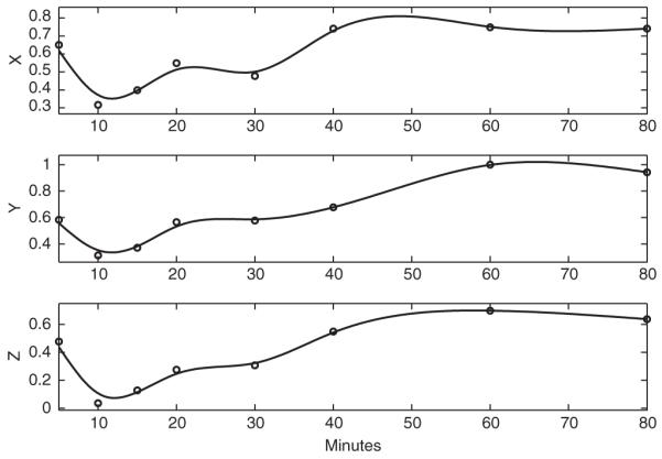
The expression profiles of three genes (X: Gene GCN4; Y: Gene LEU3; Z: Gene ILV5) measured at 5, 10, 15, 20, 30, 40, 60, 80 min. The data were collected by DNA microarrays from yeast after the temperature was increased from 25°C to 37°C (Gasch et al., 2000). The solid lines are the smooth curves estimated by penalized spline smoothing (The basis functions are cubic B-splines with 40 equal-spaced knots, and the value of the smoothing parameter is 10).

An FFL can be modeled by a set of simple first order ODEs (Barkai and Leibler, 1997; Mangan and Alon, 2003; Savageau, 1976; Shen-Orr et al., 2002). For example, the following ODEs have been used to model a Coherent Type 1 FFL:

$$\frac{\mathrm{d}Y\left(t\right)}{\mathrm{d}t}=-{\alpha }_{y}Y\left(t\right)+{\beta }_{y}f(X\left(t\right),K_{xy}),$$ (1)

$$\frac{\mathrm{d}Z\left(t\right)}{\mathrm{d}t}=-{\alpha }_{z}Z\left(t\right)+{\beta }_{z}g(X\left(t\right),Y\left(t\right),K_{xz},K_{yz}),$$ (2)

where X(t), Y(t) and Z(t) represent the expression levels of Genes X, Y and Z, respectively, at time t. The activation function f(u,K)=(u/K)^H/(1+(u/K)^H) has two parameters H and K. Parameter H controls the steepness of f(u,K), and we choose H=2 in our following analysis. Parameter K defines the expression of Gene X required to significantly activate expression of other genes. When u=K, f(u,K)=0.5. Assuming Genes X and Y regulate Gene Z independently, the activation function from Genes X and Y to Gene Z is g(t)=f(X(t),K_xz)f(Y(t),K_yz). Our objective is to estimate the vector of ODE parameters θ =(β_y,β_z,α_y,α_z,K_xy,K_xz,K_yz) from the noisy measurements for gene expression.

ODEs are popular tools to model dynamic processes in engineering, biology and many other areas. For example, in classical mechanics, the motion of a body is described in terms of its position, velocity (the first derivative of the position function) and acceleration (the second derivative of the position function) as time varies. Newton’s Laws relate the position, velocity, acceleration and forces acting on the body with differential equations. How to estimate ODE parameters is an old but difficult problem. When ODEs have analytical solutions, this is essentially a non-linear regression problem (Bates and Watts, 1988). Unfortunately, most ODEs do not have analytical solutions.

Many methods have been proposed for estimating ODEs which cannot be solved analytically. Bock (1981) proposed a multiple shooting method, which partitioned the whole time interval into segments and applied the non-linear optimization procedure over each segment. Himmelblau et al. (1967) converted ODEs to non-linear equations by integrating ODEs with numerical quadrature. de Boor and Swartz (1973) approximated ODE solutions with piecewise polynomial functions by collocation. Ramsay and Silverman (2005) estimated the derivatives of the underlying curves by non-parametric smoothing, and then estimated ODE parameters with standard non-linear regression. Huang et al. (2005) proposed a Bayesian approach by numerically solving ODEs when updating ODE parameters.

Most recently, Ramsay et al. (2007) proposed a generalized profiling method to estimate ODE parameters. The ODE solution is approximated with a linear combination of basis functions. The basis coefficients are estimated with penalized smoothing with an ODE-defined penalty. The smoothing parameter controls the trade off between fitting the data and fidelity to the ODEs. Their method has several unique aspects. For example, the computation load is much lower than the other methods because it avoids the computational expense to obtain numerical ODE solutions. The method can estimate some ODE components when they are missing. It can also estimate initial values of ODE components by evaluating the fitted curves at the first time points. Cao and Ramsay (2007) extended this method and estimated the smoothing parameter in three nested levels of optimization.

Our article is organized as follows. Section 2 introduces the generalized profiling method in details. Section 3 applies the generalized profiling method to estimate the ODE parameters in (1) and (2) from the noisy measurements for gene expression. Section 4 validates the generalized profiling method by simulations. Section 5 introduces a goodness-of-fit test for the adequacy of the FFL to model the observed expression data. Section 6 gives the conclusions and discussion.

2 THE GENERALIZED PROFILING METHOD

We start with a simple dynamic system composed of one single component, and then extend to more general cases. Let X(t) be a process modeled by one ODE dX/dt=f(X|θ), where f(X|θ) is known. We have n observations y(t_j) at a number of time points with mean X(t_j) and SD σ_j, j=1,…,n, where X(t) is the solution to the ODE over t. The parameter vector θ is unknown and has to be estimated from data y=(y(t₁),…,y(t_n)). Two nested levels of optimization are implemented. In the inner level, we approximate X(t) with a smooth curve x(t) by penalized smoothing with the ODE-defined penalty, conditional on the ODE parameter vector θ. So the fitted curve $\widehat{x}\left(t\right)$ can be treated as a function of θ. In the outer level, the ODE parameter vector is estimated by minimizing the likelihood function (the likelihood function is a function of the fitted curve, and thus is also a function of θ). The standard error for $\widehat{\theta }$ is estimated by the modified delta method, which includes the uncertainty coming from the fitted curve.

2.1 The point estimate for the ODE parameter

The ODE solution is approximated by a linear expansion of K basis functions φ_k(t),k=1,…,K, as follows:

$$x\left(t\right)=\sum _k^K{c}_k\varphi \left(t\right)={\mathbf{c}}^{\prime }\varphi \left(t\right).$$

The basis system must have the flexibility to approximate ODE solutions and their derivatives. Many dynamic systems have sharp features, such as peaks, valleys, high frequency oscillations and discontinuities in derivatives. Ramsay and Silverman (2005) showed that the B-spline basis system can accommodate the discontinuities by assigning multiple knots to the critical locations. The B-spline basis functions are only non-zero in local intervals, and the computation can be made efficient using this property of local supports. In practice, the cubic B-splines are often used as the basis system. Usually we put one knot on each point with observations, but when data are sparse or the dynamic systems have sharp features, more knots are required to make the cubic B-spline flexible enough.

The basis coefficient c is estimated by optimizing the penalized likelihood function:

$$J(\mathbf{c}\mid \theta ,\lambda ,\mathbf{y})=-l(\mathbf{c}\mid \mathbf{y})+\lambda \int {[{\mathbf{c}}^{\prime }\frac{\mathrm{d}\varphi \left(t\right)}{\mathrm{d}t}-f({\mathbf{c}}^{\prime }\varphi \left(t\right)\mid \theta )]}^2\mathrm{d}t.$$

where l(c|y) is the log likelihood function for c. The fit of the smoothing curve x(t) to the ODE is measured in the second term, which is the integrated squared difference between the two sides of the ODE. The smoothing parameter controls the tradeoff between fitting the data and fidelity to the ODE.

In general, suppose the dynamic system has G ODEs and T components:

$$\frac{\mathrm{d}{x}_g\left(t\right)}{\mathrm{d}t}=f_g(x_1\left(t\right),x_2\left(t\right),\dots ,x_T\left(t\right)\mid \theta ),g=1,\dots ,G,$$

where f_g(x₁(t),x₂(t),…,x_T(t)|θ) is known, and θ is the ODE parameter that has to be estimated. Each component is approximated by a linear combination of basis functions: x_i(t)=c_iφ_i(t),i=1,…,T. Suppose we have observations for only M≤T of these components: y_m=(y_m(t_m1),…,y_m(t_mnm)),m=1,…,M. Let $\mathbf{c}={({\mathbf{c}}_1^{\prime },\dots ,{\mathbf{c}}_T^{\prime })}^{\prime }$ and $\mathbf{y}={({\mathbf{y}}_1^{\prime },\dots ,{\mathbf{y}}_M^{\prime })}^{\prime }$ then the fitting criterion can be generalized to be:

$$J(\mathbf{c}\mid \theta ,\lambda ,\mathbf{y})=-\sum _{j=1}^M{\omega }_{j}l({\mathbf{c}}_j\mid {\mathbf{y}}_j)+\sum _{\ell =1}^G{\lambda }_{\ell }{\omega }_{\ell }\int {[{\mathbf{c}}_{\ell }^{\prime }\frac{\mathrm{d}{\varphi }_{\ell }\left(t\right)}{\mathrm{d}t}-f({\mathbf{c}}_1^{\prime }{\varphi }_1\left(t\right),\dots ,{\mathbf{c}}_T^{\prime }{\varphi }_T\left(t\right)\mid \theta )]}^2\mathrm{d}t,$$ (3)

where ω_j is the normalizing weight, which can be used to keep different components having comparable scales. For example, in this study we set the values of ω_j as the reciprocals of the variances taken over observations for the j-th component. There are sometimes some unobservable components, that is, M<T, but the basis coefficients for missing components are involved in the second term and can still be estimated. When f_g(x₁(t),x₂(t),…,x_T(t)|θ) is a non-linear function, the integration terms can be approximated by numerical quadrature. For each given value of θ, we obtain one estimate ĉ optimizing (3), so ĉ by can be viewed as a function θ.

In the outer level, we estimate the ODE parameter θ by optimizing the log likelihood function:

$$H(\theta \mid \lambda ,\mathbf{y})=-\sum _{j=1}^M{\omega }_{j}l({\widehat{\mathbf{c}}}_j\left(\theta \right)\mid {\mathbf{y}}_j)$$

We can obtain the gradients and Hessian matrices analytically, so the optimization can be fast and stable. When f_g(x₁(t),x₂(t),…,x_T(t)|θ) is a non-linear function, ĉ is an implicit function of θ, and the Implicit Function Theorem can be used to get the analytical gradients and Hessian matrices.

2.2 Statistical inference for the ODE parameter

Let Σ be the variance–covariance matrix for the data y. Ramsay et al. (2007) show that the variance estimate for $\widehat{\theta }$ can be obtained with a modified delta method:

$$\widehat{\mathrm{Var}}\left(\widehat{\theta }\right)=\left[\frac{\mathrm{d}\widehat{\theta }}{\mathrm{d}\mathbf{y}}\right]\Sigma {\left[\frac{\mathrm{d}\widehat{\theta }}{\mathrm{d}\mathbf{y}}\right]}^{\prime },$$

where $\mathrm{d}\widehat{\theta }∕\mathrm{d}\mathbf{y}$ can be derived with the implicit function theorem:

$$\frac{\mathrm{d}\widehat{\theta }}{\mathrm{d}\mathbf{y}}=-{\left[{\phantom{\mid }\frac{{\mathrm{d}}^{2}H}{\mathrm{d}{\theta }^2}\mid }_{\widehat{\theta }}\right]}^{-1}\left[{\phantom{\mid }\frac{{\mathrm{d}}^{2}H}{\mathrm{d}\theta d\mathbf{y}}\mid }_{\widehat{\theta }}\right],$$

where

$$\frac{{\mathrm{d}}^{2}H}{\mathrm{d}{\theta }^2}=\frac{{\partial }^{2}H}{\partial {\theta }^2}+2\frac{{\partial }^{2}H}{\partial \widehat{\mathbf{c}}\partial \theta }\frac{\partial \widehat{\mathbf{c}}}{\partial \theta }+{\left(\frac{\partial \widehat{\mathbf{c}}}{\partial \theta }\right)}^{\prime }\frac{{\partial }^{2}H}{\partial {\widehat{\mathbf{c}}}^2}\frac{\partial \widehat{\mathbf{c}}}{\partial \theta }+\frac{\partial H}{\partial \widehat{\mathbf{c}}}\frac{{\partial }^2\widehat{\mathbf{c}}}{\partial {\theta }^2},$$

and

$$\frac{{\mathrm{d}}^{2}H}{\mathrm{d}\theta \mathrm{d}\mathbf{y}}=\frac{{\partial }^{2}H}{\partial \theta \partial \mathbf{y}}+{\left[\frac{\partial \widehat{\mathbf{c}}}{\partial \theta }\right]}^{\prime }\frac{{\partial }^{2}H}{\partial \widehat{\mathbf{c}}\partial \mathbf{y}}+\frac{{\partial }^{2}H}{\partial \theta \partial \widehat{\mathbf{c}}}\frac{\partial \widehat{\mathbf{c}}}{\partial \mathbf{y}}+{\left[\frac{\partial \widehat{\mathbf{c}}}{\partial \theta }\right]}^{\prime }\frac{{\partial }^{2}H}{\partial {\widehat{\mathbf{c}}}^2}\frac{\partial \widehat{\mathbf{c}}}{\partial \mathbf{y}}+\frac{\partial H}{\partial \widehat{\mathbf{c}}}\frac{{\partial }^2\widehat{\mathbf{c}}}{\partial \theta \partial \mathbf{y}}.$$

The variance for ĉ can also be estimated with the modified delta method:

$$\widehat{\mathrm{Var}}\left(\widehat{\mathbf{c}}\right)=\left[\frac{\mathrm{d}\widehat{\mathbf{c}}}{\mathrm{d}\mathbf{y}}\right]\Sigma {\left[\frac{\mathrm{d}\widehat{\mathbf{c}}}{\mathrm{d}\mathbf{y}}\right]}^{\prime },$$

where

$$\frac{\mathrm{d}\widehat{\mathbf{c}}}{\mathrm{d}\mathbf{y}}=\frac{\partial \widehat{\mathbf{c}}}{\partial \mathbf{y}}+\frac{\partial \widehat{\mathbf{c}}}{\partial \theta }\frac{\mathrm{d}\widehat{\theta }}{\partial \mathbf{y}}.$$ (4)

In (4), ∂ĉ/∂y denotes the partial derivative of ĉ with respect to y, and dĉ/dy denotes the full derivative of ĉ with respect to y. Whenĉ is an implicit function of θ, ∂ĉ/∂θ can be attained with the Implicit Function Theorem. This method considers the functional relationship between c and θ, so the estimated variance for a parameter includes the uncertainty of other parameter estimates.

3 APPLICATIONS

To estimate the model parameters, we fix the value of K_xy, vary values for α_y and β_y to solve the ODE (1) with these parameter values, and calculate the sum squared differences between the ODE solution and the measured expression of Gene Y. Figure 2 displays the contour plot of the logarithms of these sums of squared differences. The optimal values of the two parameters α_y and β_y show strong collinearity, and most of them are located around the line α_y=0.11+0.15β_y. Similar conclusion can be found for α_z and β_z. So in the following, we fix the two parameters β_y=1 and β_z=1, and estimate parameters α_y,α_z,K_xy,K_xz,K_yz in ODEs (1) and (2).

Fig. 2.

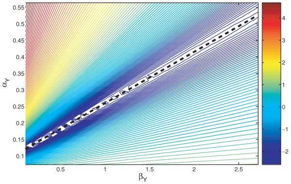
The contour plot of the logarithm of the sums of squared differences between the measured expression of Gene Y shown in Figure 1 and the ODE (1) solution with different values of α_y and β_y. The value of K_xy is fixed as 0.93. The dashed line is α_y=0.11+0.15*β_y.

We estimate dynamic models for three different FFLs—FFL 1 is composed of X: Gene GCN4; Y: Gene LEU3; Z: Gene ILV5; FFL 2 is composed of X: Gene GCN4; Y: Gene LEU3; Z: Gene ILV1; FFL 3 is composed of X: Gene PDR1; Y: Gene PDR3; Z: Gene PDR5. The expression function for Gene X, X(t), is estimated by penalized spline smoothing. We estimate parameters α_y,α_z,K_xy,K_xz,K_yz with the generalized profiling method from the measured gene expression of Gene Y and Z. Each component is approximated by cubic B-splines with 40 equally spaced knots. The smoothing parameter λ=1000. Table 1 shows the parameter estimates and their standard errors. FFL 1 and FFL 2 have the same Genes X and Y, and they are measured together in the same environmental changes (the temperature is increased from 25°C to 37°C), so the parameters for Gene Y to regulate Gene X, α_y and K_xy, have the same values. The self-regulation parameter α_z for Gene Z have different values, which means Gene Z in FFL 2 is more self-repressed than Gene Z in FFL 1. The parameter K_yz has a larger value in FFL 2 than FFL 1, so Gene Y in FFL 2 has a higher level of threshold required to significantly activate the expression of Gene Z. For FFL 3, K_xy and K_xz are relative high, which indicates that Gene X in FFL 3 has a high threshold to significantly activate the expression of Genes Y and Z.

Table 1.

Parameter estimates and the standard errors for ODEs (1) and (2) from the measured expressions of Genes Y and Z

Parameters	αy	αz	Kxy	Kxz	Kyz
FFL 1: X: Gene GCN4; Y: Gene LEU3; Z: Gene ILV5
Estimates	0.44	0.69	0.90	0.60	0.56
Standard Errors	0.22	0.18	0.33	0.06	0.15
FFL 2: X: Gene GCN4; Y: Gene LEU3; Z: Gene ILV1
Estimates	0.44	0.90	0.90	0.75	1.21
Standard Errors	0.22	0.01	0.33	0.44	0.74
FFL 3: X: Gene PDR1; Y: Gene PDR3; Z: Gene PDR5
Estimates	0.32	0.56	2.11	1.06	0.76
Standard Errors	0.15	0.12	0.74	0.32	0.21

Each component is approximated by cubic B-splines with 40 equal spaced knots. The smoothing parameter λ=1000.

In order to validate the estimates of dynamic models, it is useful to compare gene expressions to ODE solutions with the parameter estimates. To solve ODEs it numerically requires the initial values for Genes Y and Z. We estimate the initial values for Genes Y and Z by evaluating the smoothing curves at the start time point t₀=5, where the smoothing curves are estimated by minimizing penalized smoothing criterion (3). Figures 3-5 shows the numerical solutions to ODEs (1) and (2) with the ODE parameter estimates and the estimated initial values for the three FFLs. The ODE solutions are all close to the expressions of Genes Y and Z, which suggests ODEs (1) and (2) are good dynamic models for the FFL regulation network.

Fig. 3.

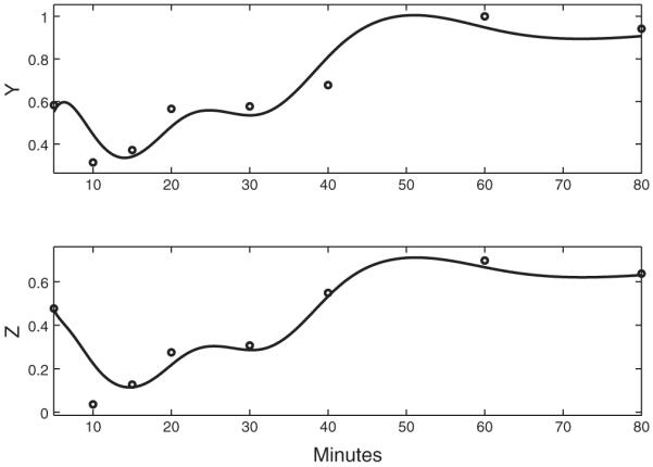
The dynamic models for FFL 1 (X: Gene GCN4; Y: Gene LEU3; Z: Gene ILV5). The circles are the real expression profiles of three genes, and the solid lines are the numerical solutions to ODEs (1) and (2) with the ODE parameter estimates α_y=0.44,α_z=0.69,K_xy=0.90,K_xz=0.60,K_yz=0.56 and the estimated initial values Y(t₀)=0.55 and Z(t₀)=0.47.

Fig. 5.

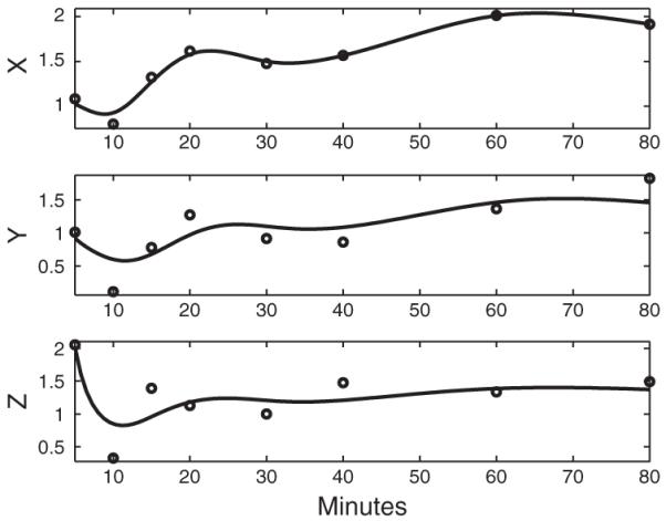
The dynamic models for FFL 3 (X: Gene PDR1; Y: Gene PDR3; Z: Gene PDR5). The circles are the real gene expression profiles of three genes. The solid lines in the top panel is the estimated X̂(t), and the solid lines in the bottom panels are the ODE solutions to ODEs (1) and (2) with the ODE parameter estimates α_y=0.32,α_z=0.56,K_xy=2.11,K_xz=1.06,K_yz=0.76 and the estimated initial values Y(t₀)=0.92 and Z(t₀)=2.02.

4 SIMULATIONS

We construct simulated data by adding Gaussian error with SD 0.1 to the solutions of ODEs (1) and (2) (shown in Fig. 4) at n equally spaced time points in [5, 80]. The true values of ODE parameters are chosen as the parameter estimates from the real data, and initial values of Y(t) and Z(t) are Y(t₀)=0.55 and Z(t₀)=0.47. The smoothing parameter λ=1000. Table 2 shows the summary of parameter estimates from 100 simulations. We choose n=10 or n=76 to explore the effect of the number of observations on parameter estimations. When we have 10 observations for each gene, the biases for parameter estimates are around 15% of the real parameter values, and the coverages of the 95% confidence intervals are above 86% for each parameters. After the number of observations is increased to 76, the biases for parameter estimates are decreased to below 4% of the real parameter values except around 10% for α_z and K_xz. The estimated 95% confidence intervals have coverage near 95%.

Fig. 4.

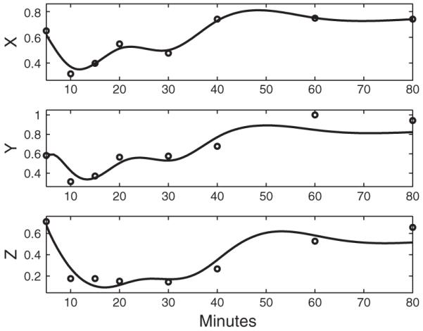
The dynamic models for FFL 2 (X: Gene GCN4; Y: Gene LEU3; Z: Gene ILV1). The circles are the real gene expression profiles of three genes. The solid lines in the top panel is the estimated X̂(t), and the solid lines in the bottom panels are the ODE solutions to ODEs (1) and (2) with the ODE parameter estimates α_y=0.44,α_z=0.90,K_xy=0.90,K_xz=0.75,K_yz=1.21 and the estimated initial values Y(t₀)=0.55 and Z(t₀)=0.70.

Table 2.

Summary of parameter estimates from 100 simulated datasets

n	Parameter	αy	αz	Kxy	Kxz	Kyz
10	True	0.44	0.69	0.90	0.60	0.56
	Mean	0.38	0.60	1.06	0.81	0.45
	Bias	−0.06	−0.09	0.16	0.10	−0.10
	STD	0.10	0.25	0.24	0.36	0.29
	Coverage	90%	87%	98%	86%	89%
76	True	0.44	0.69	0.90	0.60	0.56
	Mean	0.44	0.63	0.91	0.68	0.54
	Bias	0.00	−0.06	0.01	0.08	−0.02
	STD	0.054	0.098	0.089	0.18	0.12
	Coverage	93%	93%	93%	96%	97%

n is the number of observations for each gene.

5 TEST THE GOODNESS OF FIT OF DYNAMIC MODELS

The goodness-of-fit test of dynamic models can be used to identify whether three genes of interest compose a FFL. Since the generalized profiling method is computationally efficient (<20 s for parameter estimation for our problem), parametric bootstrap is used to test the goodness of fit of dynamic models, which is described as following. The ODE parameters θ in ODEs (1) and (2) are estimated from the expressions of Genes X, Y and Z, then we calculate the sum of squared errors:

$$\mathrm{SSE}(y,s_y,z,s_z)=\sum _{i=1}^{n_y}{[y\left(t_i\right)-s_y(t_i\mid \widehat{\theta })]}^2+\sum _{i=1}^{n_z}{[z\left(t_i\right)-s_z(t_i\mid \widehat{\theta })]}^2,$$

where y(t_i), z(t_i) are expression profiles of Genes Y and Z at t_i, and $s_y(t_i\mid \widehat{\theta }),s_z(t_i\mid \widehat{\theta })$, are solutions of ODEs (1) and (2) with parameter values $\widehat{\theta }$ at t_i. The variance for residuals is estimated as ${\widehat{\sigma }}^2=\mathrm{SSE}(y,s_y,z,s_z)∕(n_y+n_z-p)$, where p is the number of ODE parameters. Then 1000 simulated datasets are generated, and each simulated dataset, y^(j)(t_i), z^(j)(t_i), j=1,…,1000, is generated by adding Gaussian noise with variance ${\widehat{\sigma }}^2$ to ODE solutions $s_y(t_i\mid \widehat{\theta })$, $s_z(t_i\mid \widehat{\theta })$. The generalized profiling method obtain the ODE parameter estimate, ${\widehat{\theta }}^{\left(j\right)}$, from each simulated dataset. Let $s_y^{\left(j\right)},s_z^{\left(j\right)}$, be the ODE solutions with the parameter value ${\widehat{\theta }}^{\left(j\right)}$, then we can calculate the sum of squared errors, $\mathrm{SSE}(y^{\left(j\right)},s_y^{\left(j\right)},z^{\left(j\right)},s_z^{\left(j\right)})$, for each simulated dataset. The empirical P-value can then be obtained.

As one example, three genes are randomly chosen from 6152 genes in yeast (X: YLL044W; Y: YER096W; Z: YDR279W). We use the time course gene expression data measured when the temperature is increased from 25°C to 37°C (Gasch et al., 2000), which is displayed in Figure 6. The sum of squared errors from the real data to ODE solutions, SSE(y,s_y,z,s_z), is equal to 0.84. The histogram for $\mathrm{SSE}(y^{\left(j\right)},s_y^{\left(j\right)},z^{\left(j\right)},s_z^{\left(j\right)})$ is displayed in Figure 7. The parametric boostrap gives the empirical P-value 0.046, which indicates that the three genes do not compose a Coherent Type 1 FFL.

Fig. 6.

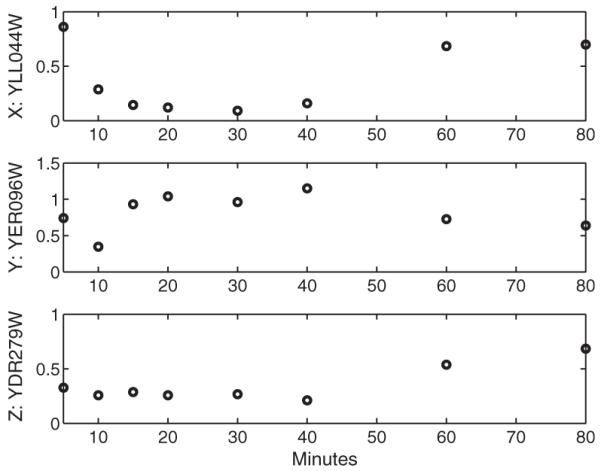
The expression profiles of three genes measured at 5, 10, 15, 20, 30, 40, 60, 80 min. The data were collected by DNA microarrays from yeast after the temperature was increased from 25°C to 37°C (Gasch et al., 2000).

Fig. 7.

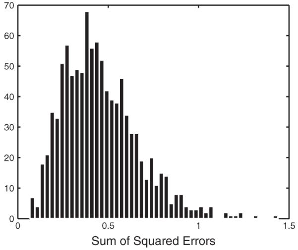
The histogram for the sum of squared errors from the simulated data to ODE solutions.

In contrast, the real data for the three sets of genes used in Section 3 are applied to test if they compose FFLs. The sum of squared errors from the real data to ODE solutions, SSE(y,s_y,z,s_z), are displayed in Table 3. The empirical P-values from the goodness-of-fit test are all much larger than 0.05, which verify that the three sets of that genes do compose FFLs. The parametric boostrap for the goodness-of-fit test is computionally intensive, which takes 11 h to finish the above example on a standard computer. Formal test statistics are required to find out all FFLs in thousands of genes, which will be addressed in the future study.

Table 3.

Identify whether three genes can compose a FFL with the goodness-of-fit test of dynamic models

Gene X	Gene Y	Gene Z	SSE	P-values
GCN4	LEU3	ILV5	0.090	0.25
PDR1	PDR3	PDR5	1.17	0.33
GCN4	LEU3	ILV1	0.092	0.34
YLL044W	YER096W	YDR279W	0.84	0.046

SSE is the sum of squared errors from the real data to ODE solutions.

6 DISCUSSION AND CONCLUSIONS

ODEs are widely used for modeling dynamic processes in engineering, biology, medicine, economics and many other areas. In this article, we propose to apply the generalized profiling method to estimate parameters in a set of non-linear ODEs for modeling gene regulation networks. The initial values for the gene expression are estimated by evaluating the fitted curves at the start time points. We show that the ODE solutions found with our estimated parameter values and initial values fit the data well. This is a good validation to show that the dynamic model can describe the observed behavior of the regulation system well. We also find two pairs of parameters show strong collinearity, an issue that can be alleviated with more observations.

Most differential equations used to model real systems are non-linear and do not have analytic solutions. Many methods for estimating ODEs have to solve ODEs numerically when searching for optimized ODE parameter values, which is computationally expensive and requires knowing the initial values of the ODE components. On the other hand, the generalized profiling method approximates ODE solutions with penalized smoothing splines, which requires a much lower computational load. A modified Delta method is developed to estimate the standard errors of the ODE parameter estimates, which takes into account the uncertainty of other parameter estimates.

Although technologies for gene expression analysis are becoming less expensive, analysis of such complex systems is still limited by the constraints on the number of microarray experiments that can be performed due to array cost and limitations of biological sample collection. We have found that some ODE parameters cannot be reliably estimated from sparse data routinely collected in microarray experiments. It is interesting to determine the frequency requirement for data collection in order to estimate ODE parameters of interest precisely. At the same time, the locations of measurement points also play an important role in the parameter estimations. This experimental design issue will be addressed in future research.

In conclusion, ODEs provide elegant models for gene regulation networks. The generalized profiling method can estimate ODE parameters quickly from noisy observations. The resulting ODE solutions using the estimated parameter values can fit the data well, which can lend evidence to the validity of the proposed ODE models.

REFERENCES

- Alon U. An introduction to Systems Biology. Chapman & Hall/CRC; London: 2007. [Google Scholar]
- Barkai N, Leibler S. Robustness in simple biochemical networks. Nature. 1997;387:913–917. doi: 10.1038/43199. [DOI] [PubMed] [Google Scholar]
- Bates DM, Watts DB. Nonlinear Regression Analysis and its Applications. Wiley; New York: 1988. [Google Scholar]
- Bock HG. Numerical treatment of inverse problems in chemical reaction kinetics. In: Ebert K, et al., editors. Modelling of Chemical Reaction Systems. Springer; New York: 1981. pp. 102–125. [Google Scholar]
- Cao J, Ramsay JO. Parameter cascades and profiling in functiona data analysis. Comput. Stat. 2007;22:335–351. [Google Scholar]
- de Boor C, Swartz B. Collocation at gaussian points. SIAM J. Numer. Anal. 1973;10:582–606. [Google Scholar]
- Gasch AP, et al. Genomic expression programs in the response of yeast cells to environmental changes. Mol. Biol. Cell. 2000;11:4241–4257. doi: 10.1091/mbc.11.12.4241. [DOI] [PMC free article] [PubMed] [Google Scholar]
- Himmelblau D, et al. Determination of rate constants for complex kinetics models. Ind. Eng. Chem. Fund. 1967;6:539. [Google Scholar]
- Huang Y, et al. Hierachical Bayesian methods for estimation of parameters in a longitudinal HIV dynamic system. Biometrics. 2005;62:413–423. doi: 10.1111/j.1541-0420.2005.00447.x. [DOI] [PMC free article] [PubMed] [Google Scholar]
- Mangan S, Alon U. Structure and function of the feed-forward loop network motif. Proc. Nat. Acad. Sci. 2003;100:11980–11985. doi: 10.1073/pnas.2133841100. [DOI] [PMC free article] [PubMed] [Google Scholar]
- Ramsay JO, Silverman BW. Functional Data Analysis. 2nd edn. Springer; New York: 2005. [Google Scholar]
- Ramsay JO, et al. Parameter estimation for differential equations: a generalized smoothing approach (with discussion) J. R. Stat. Soc. B. 2007;69:741–796. [Google Scholar]
- Savageau M. Biochemical Systems Analysis: a Study of Function and Design in Molecular Biology. Addison–Wesley; Reading, MA: 1976. [Google Scholar]
- Shen-Orr S, et al. Network motifs in the transcriptional regulation network of escherichia coli. J. Anim. Ecol. 2002;31:64–68. doi: 10.1038/ng881. [DOI] [PubMed] [Google Scholar]