Visual adaptation and novelty responses in the superior colliculus

Abstract

The brain's ability to ignore repeating, often redundant, information while enhancing novel information processing is paramount to survival. When stimuli are repeatedly presented, the response of visually-sensitive neurons decreases in magnitude, i.e. neurons adapt or habituate, although the mechanism is not yet known. We monitored activity of visual neurons in the superior colliculus (SC) of rhesus monkeys who actively fixated while repeated visual events were presented. We dissociated adaptation from habituation as mechanisms of the response decrement by using a Bayesian model of adaptation, and by employing a paradigm including rare trials that included an oddball stimulus that was either brighter or dimmer. If the mechanism is adaptation, response recovery should be seen only for the brighter stimulus; if habituation, response recovery (‘dishabituation’) should be seen for both the brighter and dimmer stimulus. We observed a reduction in the magnitude of the initial transient response and an increase in response onset latency with stimulus repetition for all visually responsive neurons in the SC. Response decrement was successfully captured by the adaptation model which also predicted the effects of presentation rate and rare luminance changes. However, in a subset of neurons with sustained activity to visual stimuli, a novelty signal akin to dishabituation was observed late in the visual response profile to both brighter and dimmer stimuli and was not captured by the model. This suggests that SC neurons integrate both rapidly discounted information about repeating stimuli and novelty information about oddball events, to support efficient selection in a cluttered dynamic world.

Introduction

Efficient selection of important events among temporal clutter requires ignoring repeating stimuli, thereby emphasizing novel and potentially important ones. This simple form of non-associative learning has been referred to as adaptation, habituation and repetition suppression, depending on the era and field of study (Clifford et al., 2007; Grill-Spector et al., 2006; Kohn, 2007; Krekelberg et al., 2006). From an information processing perspective, adaptation serves to adjust the operating point of a sensory system, to maximize the efficiency of sensory coding and increase differential sensitivity to novel events (David et al., 2004; Dean et al., 2005; Dragoi et al., 2002; Dragoi, 2002; Muller et al., 1999). This can be achieved through incremental updating over time of a Bayesian prior, which can then bias the processing of incoming sensory data (Itti and Baldi, 2005; Stocker and Simoncelli, 2006).

Electrophysiological evidence of response reduction with stimulus repetition has been observed throughout the visual system, from retina (Brown and Masland, 2001; Hosoya et al., 2005; Smirnakis et al., 1997) and thalamus (Solomon et al., 2004), to visual cortex (Maffei et al., 1973; Motter, 2006; Movshon and Lennie, 1979; Muller et al., 1999) and frontal eye fields (Mayo and Sommer, 2008). These studies usually focus on perception; however, stimulus repetition effects also have profound, though less studied, consequences on visual orienting: the latency and magnitude of the visual response influences the timing of eye and head movements to foveate the stimulus (Corneil et al., 2008; Dorris et al., 2002; Fecteau et al., 2004).

The ideal place to study visual repetition effects is the superior colliculus (SC) – the phylogenetically conserved hub of the visual orienting system (Dean et al., 1989; Huerta and Harting, 1983; Ingle, 1975; May, 2006; Munoz et al., 2000) –which is integrated with all other visual areas in the brain. Many visually responsive neurons in the SC also have movement responses time-locked to saccades (Mohler and Wurtz, 1976). The superficial layers of the SC (SCs) receive visual input directly from the retina and from early visual cortex, while the intermediate layers (SCi) receive more complex visual and cognitive input from various cortical areas, the basal ganglia and cerebellum (May, 2006). Therefore, early (e.g., retinal) and late (e.g., cortical) sources of visual adaptation can be compared directly by examining repetition effects across all SC visually-responsive neurons located in different layers.

We explored how the magnitude and onset latency of SC visual responses changed with repetition. We modeled these changes using a Bayesian approach to provide a quantitative definition of adaptation, which was then used to predict the consequences of changes to stimulus timing and intensity. To dissociate simple adaptation from higher-level learning processes (e.g., habituation), we compared responses to rarely-presented brighter or dimmer oddball stimuli. Response decrement due to adaptation should follow the adaptation model and recover with a brighter but not a dimmer stimulus; however, response decrement due to habituation should recover (dishabituation) after any novel stimulus change (Baars, 1988; Sokolov, 1963).

Materials and Methods

All procedures were approved by the Queen's University Animal Care Committee and were in full compliance with the Canadian Council on Animal Care guidelines on the care and use of laboratory animals. Experiments were performed using two male rhesus monkeys (Macaca mulatta) weighing between 9-12 kg. The surgical techniques to prepare the animal for behavioral and physiological recordings have been described previously in detail(Marino et al., 2008). Briefly, monkeys were implanted with a head post for head fixation, a recording chamber over the SC and eye coils to measure eye position with the search coil technique. The evening prior to surgery, the animal was placed under Nil per Os (NPO, water ad lib), and a prophylactic treatment of antibiotics was initiated [5.0 mg/kg enrofloxacin (Baytril)]. On the day of the surgery, anesthesia was induced by ketamine (6.7 mg/kg im). A catheter was placed intravenously to deliver fluids (lactated Ringer) at a rate of 10 mL/kg/h to a maximum of 60 mL/kg throughout the duration of the surgical procedure. Glycopyrolate (0.013 mg/kg im) was administered to control salivation, bronchial secretions, and to optimize heart rate (HR). An initial dose was delivered at the start of surgery followed by a second dose 4 h into the surgery. General anesthesia was maintained with gaseous isofluorene (2–2.5%) after an endotracheal tube was inserted (under sedation induced by an intravenous bolus of propofol, 2.5 mg/kg). HR, pulse, pulse oximetry saturation (SpO₂), respiration rate, fluid levels, circulation, and temperature were monitored throughout the surgical procedure. The analgesic buprenorphine (0.01– 0.02 mg/kg i.m.) was administered throughout the surgery and during recovery (8–12 h). The antiinflammatory agent ketoprofen (2.0 mg/kg 1st dose, 1.0 mg/kg additional doses) was administered at the end of the surgery (prior to arousal), the day after the surgery and every day thereafter (as required). Monkeys were given 2 weeks to recover prior to onset of behavioral training.

Monkeys were trained to perform a variety of oculomotor tasks for liquid reward. Real-time control of the experimental task and visual display was achieved using REX version 6.0. Monkeys were seated in a primate chair 60 cm away from a CRT monitor (Mitsubishi XC2935C, 75 Hz refresh rate, 71.5 × 53.5 cm; usable field of view of 62° × 48°). Visual stimuli were presented within a darkened environment. Dark adaptation was prevented by dimly illuminating the monitor screen for 800 ms during the inter-trial interval. Physiological activity was monitored from 109 single neurons using tungsten electrodes (Frederick Haer, 0.5-5.0 mΩ) with stimulus events and spike times collected, and waveforms digitized, through the Plexon MAP system. Further analysis was performed off-line with custom Matlab-based software.

Cell classification

When a neuron was first isolated, its visual receptive field was established using a simple fixation task in which white light stimuli (42.5 cd/m², 100 ms duration, 0.25° diameter spot) were presented in pseudorandom order to 182 possible locations distributed across 60 (horizontal) × 50 (vertical) degrees of visual angle, the order of which was designed so that no two subsequent stimuli appeared within the typical response field of a SC neuron in order to prevent adaptation effects. The centroid of the receptive field was then determined using a cubic spline function and this location was used for all subsequent study of the neuron. Because we were interested in adaptation of visual responses, we limited data collection to encountered cells that had a visual response.

We then collected further information to characterize the neuron relative to known SC cell types. First, we made careful measures of microelectrode depth referred to the dorsal surface of the SC (as determined by the electrode depth that first elicited multiunit visual-only activity). Second, neural recordings taken during four interleaved saccade tasks (step, gap, memory-delay, and visual-delay; described in detail elsewhere; (Munoz and Wurtz, 1993) were used to classify visual and motor responses; critically, the visual delay task dissociated visual and motor activity (Fig. 1A). In this task, the animal starts each trial by fixating a central fixation point (FP). A target was then presented randomly in the center of the response field or at a location opposite the vertical and horizontal meridian. To receive a reward the animal had to maintain fixation until the FP disappeared (the delay period: 500-800 ms randomized) and then make a saccade to the target.

Figure 1.

A. Raster plots and spike density waveforms (σ = 5 ms) recorded from a representative visual transient (VT), visual sustained (VS), visuomotor transient (VmT), and visuomotor sustained (VmS) neuron to a delayed saccade task, which was used to facilitate neural classification. Data are aligned on target appearance (left column) and saccade onset (right column) in the delayed saccade task when the target appeared in the neuron's response field. B. The response of the same single neurons to the 7 stimuli in the standard repetition paradigm. The black bars across bottom of abscissa represent the stimulus timing. Spikes for individual trials are presented in raster format (only a subset of trials shown for display purposes) and overlaid with a mean spike density function (σ = 5 ms). C. Scatter plots and histograms of the metrics used to classify cells. The transient-sustained index is plotted against the visual-motor index for each cell (color indicates cell class), with smaller numbers indicating a more motor and more transient responses, respectively, as measured from responses in the visual delay task shown above. The histograms show the number of cells with each parameter value using a bin width of 0.025 units. The dashed lines show the cutoff values that were used to separate classes of neurons into the 4 categories. D. The mean depth for each cell class. The cell classes had significantly unequal variances (Bartlett's test, T(3) = 15.50, p = 0.0014), and consequently a Kruskal-Wallis test was conducted to evaluate differences in depth among the four cell classes. Cell classes significantly differed in depth (C2(3, 108) = 20.10, p = 0.0002), and pair-wise Wilcoxon rank-sum tests (Bonferroni corrected) indicated that visual transient cells significantly differed from both visual motor transient and visual motor sustained (z=3.78, p < 0.001 and z=3.79, p < 0.001, respectively.).

We refer to visual responses as ‘transient’ (a short visual burst) or ‘sustained’ (visual burst followed by an extended period of low frequency activity) as was described previously (White et al., 2009). This terminology is in line with descriptions of visual neurons in the geniculostriate pathway. We classified neurons as visual transient (VT), visual sustained (VS), visuomotor transient (VmT) and visuomotor sustained (VmS, see Fig. 1B for single-unit examples) using two indices: a visual-motor index and a transient-sustained index. The visual-motor index was constructed with information from the saccade-aligned spike density function (Gaussian, σ = 5 ms) from the visual-delay task (Fig. 1A). The spike density function was first low-pass filtered by iterative convolution with a 5-tap binomial kernel: 100 iterations in the forward direction and 100 in the backward direction. The result had no phase shift and approximated convolution with a Gaussian of σ=14.12 ms. The timing and magnitude of the peaks and troughs of the waveform were then estimated by finding the zero crossings of the numerical gradient. A strong peak in activity from 25 ms pre-saccadic to 5 ms post-saccadic initiation was taken as evidence for a visuomotor neuron, and we quantified this feature with a simple probability measure:

$$P=\frac{1}{2}\left[1+\mathit{\text{erf}}\left(\frac{\theta -T}{\delta \sqrt{2}}\right)\right]$$ (1)

Where T and δ were the mean and standard deviation of non-perisaccadic peaks, θ was the value of the perisaccadic peak, and erf (x) is the Gauss error function. Large probabilities indicated the presence of motor activity, and if no peak was found, a probability of 0.0 was assigned. To confirm that the peak activity was related to a robust motor response and not to residual sustained visual activity or noise, the smallest trough was measured in a small window (±25 ms) around saccade onset. We computed the probability that activity at the trough (or at saccade initiation if no trough existed) was higher than the average pre-saccadic baseline activity (-900 ms - 50 ms pre-saccade) using Equation 1, but where T and δ were the mean and standard deviation of the baseline, and θ was the value at the trough. Finally, the visual-motor index was computed as 1 – P_pP_t, where P_p was the probability from the peak measurement, and P_t was the probability from the trough measurement. We considered cells with a visual-motor index < 0.025 to be visuomotor cells.

To compute the transient-sustained index, we aligned spike density functions to target appearance in the visual-delay task (Fig. 1A) and divided the post-stimulus visual response into early (transient) and later (sustained) components. Each time point in the first 400 ms of post-stimulus activity was compared to a baseline (700 ms pre-target) using Equation 1, where T and δ were the mean and standard deviation of the baseline, and θ was the value of the time point. Intervals of post-stimulus activity where each point in the interval had a high probability (P ≥ 0.99) were identified and if the first region had raised activity for greater than 10 ms, its start and end (maximum of 400 ms) identified the early component; otherwise, the whole post-stimulus interval from 0-400 ms was taken as the early component. The later component was then identified as the remaining interval until 550 ms after stimulus appearance (minimal delay interval). The visual-transient index was then calculated as: S / (T + S), where S was the mean activity in the later (sustained) component, and T was the mean activity in the early (transient) component. The distribution of index values for each metric is shown in Fig. 1C, To divide the cells into transient and sustained classes we chose a value of 0.2625, which was a natural division in the distribution of index values.

SC neurons have well-characterized responses ranging from purely visual to purely motor (Mays and Sparks, 1980; McPeek and Keller, 2002; Mohler and Wurtz, 1976; Munoz and Wurtz, 1995). Visual only cells with transient visual responses and no saccade-related activity (VT) tended to be located more superficially than the other classes of visually-responsive cells (see Fig. 1D). Thus VT cells were typically found in the upper superficial gray layer (e.g. SC_S), where retinal Y-type cells terminate directly and indirectly through magnocellular lateral geniculate nucleus and V1 (May, 2006). Visual-only cells that had sustained visual responses (VS) typically paused during saccadic eye movements (Fig 1A). Previously we have shown VS neurons to be sensitive to color signals whereas VT cells were not (White et al., 2009), suggesting parvocellular input. These features, along with a mean depth of about 900 μm (Fig. 1D), suggest they were located in the lower superficial layers. This area receives visual input from higher occipital and parietal areas (Graham et al., 1979; Tigges and Tigges, 1981). The VS neurons we identified were likely the same as “visual-tonic” neurons described previously (Li and Basso, 2008; McPeek and Keller, 2002). Finally, visuomotor cells with transient or sustained activity - VmT or VmS - were easily characterized because of their bursts of activity time-locked to saccades and their bursts of visual activity time locked to stimulus onset (Fig. 1A). Our sample of visuomotor neurons was by necessity biased to those with robust visual responses and were always found more than 1mm below the dorsal surface (Fig. 1D).

Behavioral Task

Monkeys actively fixated a central fixation spot (grayscale circle of 0.25° diameter presented at 1.1 cd/m²) while a series of seven light flashes (i.e., stimuli, 0.25° diameter, 55 ms duration, Fig. 1B, 2A) were presented in the receptive field of the monitored neuron. In the main paradigm, these 7 stimuli were separated by intervals of 200 ms duration (i.e., 255 ms interstimulus interval (ISI)). Monkeys received a small liquid reward for maintaining fixation within a small computer-controlled window (1-3° square window) for the duration of each trial. If fixation was broken prior to the end of the trial, the trial was aborted, eliminated from further analysis, and recycled back into the trial sequence. In the main paradigm, 70% of the trials (“Control” trials) consisted of 7 equiluminant stimuli (1.1 cd/m²) and 30% of the trials (“Oddball” trials) were identical except that the fourth stimulus could be brighter (10%, 5 cd/m²), dimmer (10%, 0.1cd/m²), or absent (10% of trials). These trial types were randomly interleaved. Trains of 7 stimuli were chosen because they allowed for examination of responses before and after presentation of the oddball, and it was a comfortable trial duration for the monkey to maintain steady fixation. The ISI of 255 ms was chosen because maximal inhibition of return was observed in monkeys at a cue-target onset asynchrony of that interval (Fecteau et al., 2004).

Figure 2.

A. Spike density functions for visual transient (VT, n = 32), visual sustained (VS, n = 32), visuomotor transient (VmT, n = 16), and visuomotor sustained (VmS, n = 18) neurons in response to 7 repeated stimuli (shown as small dark bars at bottom of trace) in the center of each neuron's response field. B. Color coding of intensity of neural activity in response to the 7 stimuli (time of the response to a given stimulus on the horizontal, response to each stimulus descending vertically, color coded for normalized spike rate). Note the shift in onset latency with each stimulus repetition. C. Changes in mean response onset latency across stimulus number for each neural type. D. Changes in peak response magnitude across stimulus number for each neural type, normalized to the response on the first stimulus. E. Population spike density waveforms in response to the first target stimulus, aligned on response onset to show the early (transient) and later (sustained) components of the visual response. F. Normalized mean sustained activity (50 ms to 100 ms after onset of visual response) is plotted for the 7 stimuli for VS and VmS neuron populations. G,H. Scatter plots showing the relationship between the response to the first and second stimulus for the transient peak (G) and sustained portion (H) of the neural response. Standardized major axis regression analysis revealed that this relationship had a slope greater than unity for the peak activity (F test, F(1,96)=72.32, p < .01), but not for the sustained activity (F test, F(1,48)=0.99, p = 0.32).

For a subset of neurons (N = 19 tested and 17 analyzed, 2 removed for having no response to some stimuli), the ISI was varied systematically between 155, 255, or 455 ms in the control condition only, to investigate the effects of ISI on the repetition effect. Typically the 255 ms ISI block was collected first because that was part of the main paradigm used with the oddball trials. If neuronal isolation remained strong after that paradigm, additional files were obtained at other ISIs collected in pseudo random order.

Neural Analysis

Single neurons or pairs of single neurons were recorded from a single electrode, isolated online using the window discriminator in Plexon, and verified and optimized offline using Plexon's Offline Sorter. The timing of events in the trial sequence was then calculated automatically using custom Matlab (Matlab 6.1 Mathworks Inc) software during offline analysis. We recorded from a total of 109 neurons in the control task with oddball trials. Of these, recordings from 98 neurons (60 from monkey Q, 38 from monkey Y) had sufficiently good spike isolation throughout recording, a mean visual response greater than 40 spikes/sec, responses to all 7 stimuli during the control trials, and at least 6 trials of each oddball condition. Typically, there were 10-20 repetitions of each oddball condition and 70-140 repetitions for the control condition. Two spike density functions were created for each trial of each condition by convolving the trains of action potentials with a Gaussian kernal (σ = 5) or by convolving with a combination of growth and decay functions that resemble a postsynaptic potential given by:

$$R(t)=(1-e^{-t/{\tau }_g})(e^{-t/{\tau }_d})$$

where R is the firing rate as a function of time t, τ_g is a time constant for the growth phase, and τ_d is a time constant for the decay phase. Time constants of 1 and 20 for the growth and decay phases, respectively, were chosen following others (Thompson et al., 1996). Spike density functions were aligned on the first stimulus onset and activity from repeated trials were averaged to generate a mean spike density function (for both functions separately) for each neuron for each condition. The magnitude of the first peak response to each visual stimulus was calculated off the Gaussian spike density function and the onset of that response was calculated from the spike density function created by rate function R, which provides a more accurate measurement of onset time. This was done for the responses to each of the 7 stimuli in every condition, for each neuron. To find the first peak in the visual response and its onset, a custom computer algorithm written in Matlab looked for all peaks in the spike density function in the epoch from 50 ms after stimulus onset until end of the ISI. It then marked the highest peak (usually the first one) on a visual display. Each first peak calculation was manually examined and changed if it was incorrect (e.g., if a late noisy peak was incorrectly chosen as the first main peak by the algorithm). Once the peak was determined, the onset latency of that visual response was calculated by an algorithm which looked backward in time (maximum of 40 ms back) along the descending slope from the first peak in order to find the point at which the response became significantly greater then the mean neural activity in an epoch spanning 25 ms before to 25 ms after the onset of the visual stimulus that generated that response. Again, these were each examined on the visual display, and manually adjusted if necessary (e.g., if unusual noise levels, or sustained activity from the preceding response unduly lengthened the ROL calculation of the algorithm).

ROC Analysis

The receiver operating characteristic (ROC) was used to quantify the time course of differences between control and oddball conditions after the presentation of the 4^th stimulus in the sequence. For each cell we computed the area under the ROC curve between the control condition and each oddball condition in a 50 ms sliding window centered on the time point of interest (gray box bottom left of Fig. 6A). The window's left edge started at the onset of the visual response and advanced 1 ms in time (depicted by the solid line) until the right edge reached the onset of the next (5^th) stimulus. This resulted in one ROC area measurement for each cell and each time point on the interval shown (which started at ½ the window size, 25 ms after the onset of the visual response). To control for variation in timing of each cell's response to the 4th stimulus, it was necessary to first align each spike density function to the onset of visual activity to the 4th stimulus. As a result of this realignment the waveforms from different neurons and conditions had slightly different lengths since the time of the visual onset varied depending on cell type and condition, and consequently, the ROC analysis was performed over a different length of time for each cell and condition. As a result, fewer cells entered the ROC area calculation near the end of the analysis interval. The length of the analysis interval shown in Fig. 6 (below VT spike density function) was the maximum interval that could be chosen that still contained greater than 50% of the cells for all classes and conditions (all but visuomotor transient cells had more than 80% at the end of this interval). All cells in all conditions had at least 122 ms from the onset of the visual response to the onset of the next stimulus, and the median was 152 ms.

Figure 6.

Changes in the later sustained part of visual response to oddball stimuli presented in the 4^th stimulus position are shown for each neuron type A: VT; B: VmT; C: VS, D: VmS. An ROC analysis was performed to determine at what points in time the later (sustained) part of the visual response became significantly different between control trials and either brighter or dimmer trials. The overlaid spike density functions show the average activity for the control, brighter, and dimmer conditions aligned to the onset of the transient visual response (see Methods) to the 4th stimulus. The filled colored regions represent the standard error of the ROC area across all cells of the same class, for the brighter and dimmer conditions separately. A ROC area of 0.5 or less indicates no difference between the control and oddball conditions at that particular time point, while values greater than 0.5 indicate the oddball condition had more activity on average. Each point was tested with a 1-tailed t-test to determine if the ROC area was significantly greater than 0.5. The p-value of this test is plotted below each ROC area plot and the vertical dotted lines and light gray shaded regions indicate when the p-value crossed the significance threshold (p<0.05). All ROC area's for all time points were normally distributed (Kolmogorov–Smirnov, p<0.05). E. Scatterplot of the mean sustained activity for the 4^th stimulus in control trials vs. mean sustained activity in the brighter or dimmer oddball stimuli for VS neurons. Inset graph shows the population mean sustained activity with standard error bars for the control, brighter and dimmer stimuli. Asterisk shows significant difference between oddball and control activity rates (paired t-test, 1-tailed). F. As described in E, but for VmS neurons.

Implementation of the computational model

The Bayesian model of adaptation is summarized in Fig. 3A. The model is based on Surprise theory using a Poisson-Gamma model which is described in detail elsewhere (Baldi and Itti, 2010; Itti and Baldi, 2005) but summarized here noting differences in our implementation. The model consists of two stages of Bayesian learning which are identical except for their input sources (Fig. 3A), so for clarity the equation subscripts are omitted from the following discussion. We consider that each Bayesian learner receives 1-dimensional Poisson-distributed spike trains (from the retina and visual cortex or from the previous stage of learning) represented internally as a family of models, M(λ), which are all the possible 1-dimensional Poisson distributions of firing rates (λ > 0). Each learner builds probability distributions (hypotheses or beliefs), P(M(λ)), about which of these models best represents the current state of the stimulus. As is typical in iterative Bayesian learning, the prior and posterior are chosen from the same functional form (conjugate priors) so that the posterior at one time step is used as the prior for the next. When the data is Poisson-distributed (D = λ) the Gamma probability density function is the conjugate prior, P(M(λ)):

Figure 3.

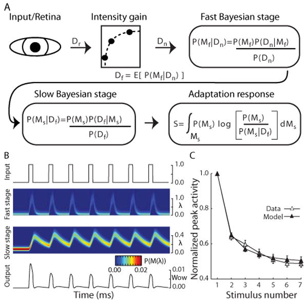
A. Schematic of the Bayesian adaptation model. Light stimulating the retina was modeled as a square wave of unity amplitude (D_r; 1.1 and 0.9 for the brighter oddball conditions) and passed through a static gain function that was constant for all model neurons (see Methods). Two stages of Bayesian learning supply the adaptation dynamics. In each stage (subscripts omitted), the learning process builds hypotheses or beliefs (probability distribution) over a class of internal models M that represent all possible values of its input. As new sensory data D_r is collected, Bayes theorem provides the mechanics to turn a prior set of hypotheses P(M) about which model best characterizes the input data into a posterior set of hypotheses P(M|D), given the likelihood of the data P(D|M) under the assumptions of model M. The fast Bayesian stage quickly adapts to the input and passes the expectation of its posterior beliefs D_f as input to the second Bayesian stage. A posterior set of beliefs is computed in the same fashion as the fast learner, but with a slower learning dynamic. The adaptation response is then calculated for every data observation as the Kullback-Leibler (KL) divergence (Kullback, 1959) between the slow learner's prior and posterior hypotheses, signaling the amount of shift in the model's beliefs caused by each new observation. B. Detailed view of the model dynamics across each stage during a control trial (see methods for a detailed description of the model). Top trace represents the input stimulus from control trials. The two central images show, for each Bayesian learner, the distribution of beliefs about which of the possible Poisson firing rates (y-axis) best characterizes the input over the course of a single trial (x-axis). Hotter colors indicate that, at a given point in time, there is a higher belief (probability) in a particular firing rate. The bottom panel shows the final output of the system. C. Population mean and standard error of the model (filled symbols) and neural (open symbols) normalized peak responses to the 7 stimuli in the control condition.

$$P(M(\lambda ))=\gamma (\lambda ;\alpha ,\beta )=\frac{{\beta }^{\alpha }{\lambda }^{\alpha -1}{e}^{-\beta \alpha }}{\Gamma (\alpha )}$$ (2)

with shape α > 0, inverse scale β > 0, and where Γ(α) is the Euler Gamma function of α. Given an input sample D = λ, the posterior distribution of beliefs over the possible input firing rates is also a Gamma distribution characterized by:

$$\alpha \prime =\zeta \alpha +\lambda +\varepsilon \text{and}\beta \prime =\zeta \beta +1$$ (3)

where α′ and β′ are the shape and inverse scale of the posterior distribution, ζ is a temporal parameter (forgetting factor, 0 < ζ < 1) which determines the rate of learning, and ε is a constant representing noise. The second stage of Bayesian learning takes as input the expected value of the first stage's posterior distribution:

$$E[P(M(\lambda )|D)]=E[\gamma (\lambda ;\alpha ,\beta )]=\frac{\alpha }{\beta }$$ (4)

The output of the system is then calculated from the final Bayesian learner as the Kullback-Leibler divergence (Kullback, 1959) between prior and posterior distributions over all possible firing rates, which summarizes the amount of learning or adaptation which just resulted from observing the data D:

$$KL(P(M(\lambda )),P(M(\lambda )|D)=KL(\gamma (\lambda ;\alpha ,\beta ),\gamma (\lambda ;\alpha \prime ,\beta \prime ))=\alpha \prime log\frac{\beta }{\beta \prime }+log\frac{\Gamma (\alpha \prime )}{\Gamma (\alpha )}+\beta \prime \frac{\alpha }{\beta }+(\alpha -\alpha \prime )\Psi (\alpha )$$ (5)

where Ψ(α) is the digamma function of α. This differs from the Itti & Baldi implementation (Baldi and Itti, 2010; Itti and Baldi, 2005) where the KL divergence is computed at each learning stage, and the system output is the product of the outputs at each stage. Fig. 3B shows the time dynamics of the system for each stage in response to a control trial.

The Itti & Baldi implementation uses five learning stages each having the same temporal parameter. In this experiment we found that only two stages, but allowing each stages temporal parameter to be different, adequately predicted the peak firing rates of the neurons. Additionally, in their implementation of Equation 3 the temporal parameter is applied to the prior distribution's α and β parameters before computing the Bayesian update. As a result, there is always a baseline output. We computed the update so that if the posterior and prior are the same, the output of the system is 0.

Model Fitting

Model parameters were estimated for each neuron individually by fitting the peaks in the model's output to the seven peak magnitudes in each neurons response profile from the ISI 255 ms condition. Each model neuron consisted of three parameters: two time constants (ζ, eq, 3) that controlled the speed of learning in the two Bayesian learners and the baseline noise parameter (ε, eq. 3) which was globally set for all model neurons. The data were fit initially with all three parameters free for each cell. After fitting, a probability density function of the baseline parameter was estimated using kernel density estimation with automatic bandwidth selection (Sheather and Jones, 1991), which was implemented in the R statistical package. A quadratic function was fit (least squares method) to 3 points centered on the maximum of this curve, and the analytic maximum of the quadratic function was used as an estimate of the most likely value of the baseline parameter. Fitting was then performed again with the baseline parameter fixed for all cells to the most likely value, reducing the model to the two temporal parameters. The best parameters were determined by using the Nelder-Mead simplex method (Lagarias et al., 1998) built into Matlab to minimize the error of the following process: First the input signal (7 stimuli) was simulated as a square wave with unit amplitude and the adaptation model's response was computed for a given parameter set. Parameters were encoded such that the second stage's learning rate was guaranteed to be slower than the first stage's. Model and cell responses were normalized by the response to the first stimulus. Normalization eliminated the need for scaling parameters in the model without affecting the morphology of the adaptation. The error was then computed as the median absolute difference between the model's peak response to each stimulus and the cell's peak responses (disregarding the first stimulus which always had zero error). Several alternative error functions were explored, and median absolute error was chosen because it gave highly significant, and qualitatively the best, overall fits and predictions. Several other error functions also gave significant results. Additionally, a single-parameter model significantly fit the data; however, the two-parameter model produced less total error for all conditions combined, and less median error for all but the 155 ms ISI condition. Qualitatively, the mean population responses of the neural data were in agreement with the mean population responses of the two parameter model.

To account for the relationship between stimulus brightness and a cell's peak firing rate, the adaptation model used a gain function (Fig. 3A). Because only three intensity levels were considered, this amounted to finding two gain factors to represent the 10% brighter and 10% dimmer stimulus. After finding the best temporal parameters during control trials, a single set of gain parameters was chosen that minimized the error between all model neurons and all real neurons simultaneously, only considering the brighter and dimmer conditions. For this data set, the gain factors were ∼1.1 and ∼0.9, respectively. Because the gain factors were very close to the 10% brighter and 10% dimmer input, the gain function could have been omitted with little loss of model fit quality.

Model Evaluation

To evaluate the model fits without assumptions about the distribution of data or errors, several statistics were computed in the permutation (randomization) framework. Goodness-of-fit was assessed by using the median of the absolute error between all neuron and model responses, for all conditions, as a test statistic in a repeated measures permutation design (stimulus 2 to 7 for each condition). To assess whether cell and model responses came from the same underlying distribution, the permutation equivalent of a two-factor repeated measures ANOVA was performed. The final test (paired-error or reliability test) indicated whether, overall, the model was able to predict neuronal responses better than other cells from the same class (which might be thought of as an upper-bound). First, for each condition separately, all pairwise combinations of neurons (restricted to within neuron class) were evaluated with the error function. This distribution of values represents the errors that occurred when each cell was used to predict other cell responses, and served as a summary of the variability (reliability) of the repetition effect within a class of neurons. Higher values indicated that neurons responded very differently from one another. Using the permutation equivalent of a two-factor repeated measures ANOVA, this distribution was compared to the distribution of errors generated by model predictions. Figures 4D, and 5C show the distribution of model errors for the ISI, and oddball manipulations, respectively. This test compared directly the quality of our model fits to the variability of the repetition effect. We reason that a well performing model should be on average as, or more, consistent with the neurons' response than neurons of the same class are with each other. All permutation tests were carried out using the Monte Carlo method with 30,000 iterations.

Figure 4.

Effect of changing interstimulus interval (ISI) on the repetition effect. A. Population spike density waveforms recorded from 17 visually responsive neurons in the SC in response to 7 stimuli (55ms) presented with ISIs of 155, 255, 455 ms. As ISI increased, the repetition effect was reduced. At short ISIs the response onset latency (B) was increased and peak response magnitude (C) was decreased with stimulus repetition. Without changing the parameters used to generate the model fit to control trials (Fig.3c), the model (closed symbols) predicted the neurons peak response magnitude (open symbols) across the different rates of stimulus presentation (two-factor repeated measures permutation-test, p = 0.89). D. The paired-error test (see Methods) indicated that, on average, each model was a better predictor of the peak activity of its corresponding real neuron, than other neurons of the same class (p<0.01). Histograms of median absolute errors between each neuron and its corresponding model for the three ISI conditions are shown in (d). The black dot and line below each axis show the median error and 95% bootstrapped confidence interval (30,000 iterations) of model errors. The gray dot and line show the median error and 95% bootstrapped confidence interval from the distribution of pairwise errors between actual neurons (see Methods). Notice that in all cases the models' median error is less than the median error between neurons.

Figure 5.

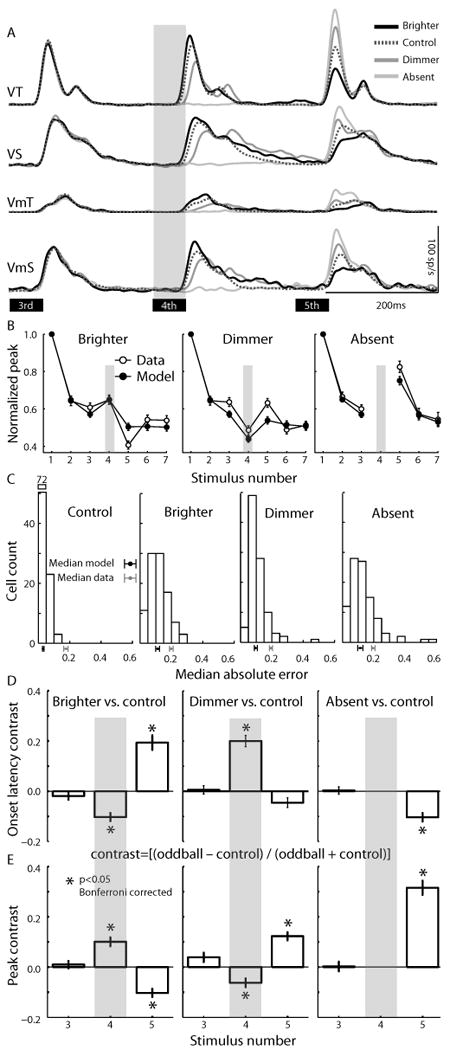
Changes in the early transient part of visual responses to oddball stimuli presented in the 4^th stimulus position in the sequence as depicted by the gray shaded bar across the different panels. A. Population spike density waveforms showing the response to the 3^rd, 4^th and 5^th stimuli are plotted for the 4 classes of visually responsive neurons studied (same neurons as Fig. 2). B. Changes in the normalized peak response magnitude across stimulus number for model (closed symbols) and neural responses (open symbols) were not significantly different (two-factor repeated measures permutation-test, p=0.61). The paired-error test (see Methods) indicated that, on average, each model was a better predictor of the peak activity of its corresponding real neuron, than other neurons of the same class (p<0,01). Histograms of median absolute errors between each neuron and its corresponding model for the control and oddball conditions are shown in (C), conventions are the same as in Fig. 4d. Mean normalized difference (i.e., contrast) in ROL (D) and mean normalized difference in peak response magnitude (E) between the control condition and each oddball condition calculated as [(control-oddball)/(control + oddball)]. Negative and positive values mean that oddball conditions had lower and higher values respectively compared with control conditions.

Results

Effects of stimulus repetition

Figure 2 illustrates the main effect of this study – the large response decrement that occurred with repeated stimulation (7 stimuli) of the receptive field of visually-responsive neurons in the SC. Response decrement was observed for all four types of visual neurons classified: visual transient (VT, n=32), visual sustained (VS, n=32), visuomotor transient (VmT, n=16), and visuomotor sustained (VmS, n=18) neurons (see Fig.1B for examples of individual neuron responses). Following the appearance of the first stimulus, neurons of each cell type discharged a robust phasic response (Fig. 2A, E). The early transient part of this response was dramatically affected by repeated stimulation: the peak response magnitude decreased (Fig. 2A, B, D) and response onset latency (ROL) increased (Fig. 2B, C). A mixed analysis of variance (ANOVA) with a between-subjects factor (4 cell classes) and a within-subjects factor (7 stimuli) was conducted which revealed significant main effects of cell class [Peak: F(3,94)=9.15,p<0.01; ROL: F(3,94)=8.8, p<0.01], stimulus repetition [Peak: F(6,94)=378.1,p<0.01; ROL: F(6,94)=89.9, p<0.01] and an interaction [Peak: F(18,564)=5.8, p<0.01; ROL: F(18,564)=3.3, p<0.01].

All cell types decreased their peak response magnitude with repetition (Peak: VT [F(6,186)=143.06,p<0.001]; VS[F(6,186)=71.69,p<0.001)]; VmT[F(6,90)=114, p<0.001)]; VmS[F(6,102)=71.5,p<0.001)] and the majority of the decrease occurred on the second stimulation. This was verified statistically: the ratio of peak magnitude between the 1^st and 2^nd stimuli (mean= 0.36) was greater than the ratio of peak magnitude between the 2^nd and 7^th stimuli (mean=0.15) [t(97)=7.9, p<0.001; paired t-test]. This relationship was confirmed for all cell types independently (p=0.04 or less). ROL increased in a mostly linear fashion with repetition for all cell types (VT [F(6,186)=18.1,p<0.001]; VS[F(6,186)=42.5,p<0.001)]; VmT[F(6,90)=15.9, p<0.001)]; VmS[F(6,102)=17.5,p<0.001)].

In summary, VT neurons, likely found in the most superficial retino-recipient SC layers (May, 2006), had strong adaptation (∼50%) but the smallest ROL increase (∼10 ms) of all cell types. VS neurons, likely found in lower superficial layers (Tigges and Tigges, 1981) showed the least adaptation (∼35%) but a large increase in ROL with repetition (∼15 ms). Finally, Vm neurons of the intermediate SC layers showed both strong adaptation (>50%) and a large increase in ROL (>15 ms), particularly the VmT cells. Indeed some VmT cells (not described here) completely lost their visual response after only a few trials (Goldberg and Wurtz, 1972) and thus could not be studied in our paradigms.

To determine whether the later components of the visual response in cells with a significant sustained component (VS and VmS as defined by our cell classes) were also affected by repetition, we calculated the average activity from 50-100 ms after the response onset (Fig. 2E). The sustained activity was less affected by repetition (Fig. 2F, H) than the early transient component (Fig. 2D, G). An ANOVA on the sustained activity of VS and VmS neurons showed a far smaller main effect of repetition [F(6, 48)=6.75, p<0.01] compared with that seen in the transient component, and no main effect of cell class, nor an interaction (F's<1).

Modeling the response decrement using a Bayesian framework

The effect of stimulus repetition on response magnitude was modeled using a simple Bayesian model of stimulus adaptation which monitored the temporal dynamics of streams of stimuli (see Fig 3A, B, and Methods). The model relies on a recently developed Bayes-optimal theory of novelty, shown to provide a quantitative account of adaptation in early visual neurons (Baldi and Itti, 2010; Itti and Baldi, 2005) This model provided a principled theoretical foundation for quantifying the effects of adaptation in terms of a hypothetical optimal Bayesian learner: stimuli that over time gave rise to no significant learning caused a rapid decrease in response (adaptation); in contrast, stimuli that caused a shift in the model's current estimates gave rise to significant learning and to vigorous model responses. Each neuron was modeled individually as three stages consisting of a static gain function and two Bayesian learners (Fig. 3A). Parameters were estimated by fitting each model neuron's peak responses to a real neuron's peak responses to all seven stimuli (see Methods). The model was able to significantly fit the repetition effect (goodness-of-fit test, p<0.01), and the population responses for model and real neurons overlapped (Fig. 3C).

The effect of stimulus presentation rate

We generated predictions for the repetition effect's dependence on the rate of stimulus presentation by altering the inter stimulus interval (ISI) of inputs to the population of model neurons. If the response decrement followed the adaptation model predictions then decreasing the ISI to 100 ms would cause a stronger repetition effect, while increasing the ISI to 400 ms would allow recovery of the effect of previous stimulation. We tested these predictions in a subset of 17 neurons (3 VT, 7 VS, 3 VmT, 4 VmS) by repeating control trials (7 identical stimuli of 55 ms duration) with these different ISIs (onset to onset time = 155, 255 and 455 ms). Figure 4A shows the combined spike density functions from this subpopulation. There was a clear effect of ISI on both peak response magnitude [F(2,32)=29.14, p<0.01)] and ROL [F(2,32)=28.5, p<0.01]. That is, the shorter the ISI, the more dramatic the repetition effect. This was confirmed by an interaction between ISI and repetition [Peak: F(12,192)=8.44, p<0.01; ROL: F(12,192)=6.9, p<0.01]. Reducing ISI led to an increase in ROL (Fig. 4B), and a reduction in response magnitude (Fig. 4C). The main effect of repetition, as expected, was significant [Peak: F(6,96)=46.29, p<0.01; ROL: F(6, 96)=32.27, p<0.01]. Remarkably, we found that our simple model was able to predict the pattern of response magnitudes observed in these other ISI conditions (Fig. 4C) without a change in parameters (goodness-of-fit test, p<0.01) and was a better predictor of neural activity than other neurons (see Fig.4D).

The effect of rare changes in stimulus luminance

We also modeled the effect of inserting rarely presented luminance oddball stimuli (brighter, dimmer, absent) into the stimulus sequences. If the pattern of changes were due purely to adaptation, the neural response should follow the predictions of the adaptation model and recover somewhat with a brighter stimulus, but not a dimmer stimulus, and have an opposite trend on the stimulus following the oddball. Alternatively, neurons could show response recovery to all the rare stimuli, akin to ‘dishabituation’. To test these predictions, we examined the visual response of SC neurons to sequences of 7 stimuli where the 4^th was of higher intensity (10% of trials), lower intensity (10% of trials), was absent (10% of trials), or had no change (70%). Figure 5A illustrates the population responses recorded from each type of neuron for the 3^rd, 4^th and 5^th stimuli. We found that the peak magnitude of the neural data conformed to the predictions of the adaptation model using the same parameters as in the control condition (see Fig. 5B to contrast physiological data with model fits). The model fit the data significantly (goodness-of-fit test, p<0.01), and was a better predictor of neural activity than other neurons in the same class (Fig. 5C).

Figure 5 D and E show the normalized difference [(oddball – control) / (oddball + control)] between the oddball and control trials for ROL and the peak magnitude, respectively (all cell types were collapsed because the changes in the early part of the visual response were qualitatively the same in all cell types). Significance was tested using a Bonferroni corrected t-test (critical t = 2.49, p<0.05). As expected, there was no difference between control and oddball trials on the 3^rd stimulus for any condition (all t's < 2.49). Presentation of the brighter stimulus in the 4^th position led to a larger magnitude response [t(97)=5.67] at a shorter latency [t(97)=-6.36], while presentation of the dimmer stimulus showed the opposite effect – smaller peak response [t(97)=-3.7] with a longer latency [t(97)=8.79]. Furthermore, the changes in the latency and magnitude of the 4^th response had predictable consequences on the earliest part of the response to the 5^th stimulus. If the 4^th stimulus was brighter, the response to the 5^th was reduced [t(97)=-6.22] and arrived later in time [t(97)=6.72] compared to the control condition. In contrast, when the 4^th stimulus was dimmer, the response to the 5^th stimulus was larger in magnitude [t(97)=7.6] but not significantly earlier in time [t(97)=-2.36]. In the absent 4^th stimulus condition, the response to the 5^th stimulus was much larger in magnitude [t(97)=11.24] and occurred earlier in time [t(97)=-6.02]. These analyses indicate that the pattern of changes observed in the timing and magnitude of the early transient component of the response to oddball stimuli are consistent with predictions of Bayesian adaptation to stimulus intensity.

Sustained responses to novel events

The best fitting adaptation models often did not produce any output during the inter trial interval (sustained response), but a sustained response that showed some modulation to repeated stimuli was observed in sustained cell classes (Fig. 2E,F). To investigate whether the sustained activity could possibly reflect something other than simple adaptation, we analyzed the later part of the visual response to oddball trials (Fig. 6). First, we realigned the visual responses in control and oddball conditions to the onset of the response to the 4^th stimulus (see traces on left side of each panel in Fig. 6), correcting for the ROL difference between brighter and dimmer stimuli and between cells (Fig. 5D). We then performed a receiver operating characteristic (ROC) analysis on the response spanning from 25-120 ms after response onset (right side of each panel in Fig. 6) to determine when the response to the control and oddball trials became significantly different (see Methods). This analysis interval started earlier than that used in Fig.2 to show the effect of the first visual volley in the ROC plots. For all cell types except VmT, immediately after the onset of the visual response there was a significant difference in the transient response in the brighter condition that became insignificant approximately 30 ms after the ROL. That is, the peak transient activity faithfully reflected stimulus intensity - the brighter stimulus elicited the strongest response, the dimmer stimulus the weakest. However, later in the response of the VS and VmS cells (bottom panels), there was a significant increase in activity for both the brighter and dimmer oddball conditions, possibly representing a dishabituation signal reflecting the novelty of the oddball stimuli. The time point after ROL when the brighter and dimmer stimulus responses diverged from control responses was at 73 ms and 68 ms, respectively, for VS neurons, and 95 ms and 81 ms, respectively, for VmS neurons (see vertical dotted lines, and p-values plotted below the ROC area curves). To demonstrate how consistent this was across individual neurons, in Fig. 6, E-F the mean sustained firing rate after the 4th stimulus for control trials is plotted against that for oddball trials for VS and VmS neurons respectively. Points falling above the unity line show neurons whose rate was higher after the oddball stimulus vs. control stimulus (sustained epoch 80-110 and 90-120 for VS and VmS neurons respectively). In the inset graphs we show the grand mean firing rate with standard error bars for the control and oddball stimuli. The rate for oddball stimuli was signficantly greater than control for each comparison (paired t-tests, 1-tailed; all p's <0.002) There was no change in the later portion of the visual response for VT and VmT neurons (Fig. 6, A-B).

In sum, the oddball manipulation shows that the pattern of effects seen in the peak of the transient response was consistent with the adaptation to light intensity computed by our model; however, a significant dishabituation signal (enhanced response to both brighter and dimmer stimuli) not seen in the model response was present in the later part of the visual response only in neurons with sustained activity.

Discussion

The timing and magnitude of the visual response of SC neurons underwent significant modification following stimulus repetition: the earliest part of the visual response decreased in magnitude and increased in latency with repetition (Fig.2). The modulation of this early response with repetition was successfully modeled using our Bayesian adaptation model (Fig.3) and predictions made about the effect of changing the rate of stimulus presentation (Fig.4) and the intensity of rare stimuli (Fig.5) were confirmed with neural data. The repetition effect was strongly dependent on the rate of stimulus presentation (Fig. 4), with the repetition effect increasing in magnitude as the interval between stimuli was reduced. For brighter or dimmer oddball stimuli, the main features of the repetition effect followed simple adaptation to light – larger, earlier responses to the brighter, and smaller, later responses to the dimmer oddball stimuli and the opposite pattern in response to the next (non-oddball) stimulus. In contrast, the later, sustained component of the visual response was modulated much less by repetition, as observed previously in V4 (Motter, 2006), and was inconsistent with our Bayesian adaptation model. Finally, in response to either brighter or dimmer oddball stimuli we observed an increase in response (e.g., a dishabituation) in this later sustained firing, suggestive of a “novelty response”.

Comparison to other studies

Reductions in response magnitude with repetition have been previously observed in cortical areas including V1 (Muller et al., 1999), V4 (Motter, 2006) and frontal eye fields (Mayo and Sommer, 2008), and also in single neurons of the SC (Goldberg and Wurtz, 1972; Woods and Frost, 1977) and multi-unit activity of the SCs (Mayo and Sommer, 2008). In the context of an attentional cueing task, a repetition effect has been described in the SC (Bell et al., 2004; Dorris et al., 2002; Fecteau et al., 2004; Robinson and Kertzman, 1995) and LIP (Robinson et al., 1995). The present report is the first to systematically explore the repetition effect using long stimulus sequences studied across different cell types and layers in the SC, the first to report the increase in response onset latency with repetition in the SC, and the first to explore the mechanism for this response decrement through modeling and experimental manipulations (oddball stimuli).

We observed a significant increase in ROL with repetition and with changes in stimulus intensity (oddball experiment). Modulation of ROL with intensity is consistent with previous reports on intensity modulations in the SC(Bell et al., 2006; Li and Basso, 2008). Increases of ROL with stimulus repetition are evident in some results from V4 (Hudson et al., 2009; Motter, 2006), although have not been explicitly described in the SC. There is one study in the SC which did not show an ROL increase with repetition (Mayo and Sommer, 2008) and there were interesting stimulus differences between their study and the present one that may explain why: the two stimuli in their sequence were shifted spatially in order to activate different retinal receptive fields but the same relatively large receptive fields in the frontal eye fields or SCs. Thus, their failure to see the ROL increases with repetition, while observing the decrease in response magnitude, may suggest that the ROL effect occurs very early in visual processing (e.g., retina, lateral geniculate nucleus of the thalamus or input to V1) while the magnitude decrease occurs more centrally (e.g., V1 or beyond), although the anatomical locus of these effects remain to be explicitly tested. There are a few possible explanations for the ROL increase: there could be a complete elimination of the earliest spikes of the response due to adaptation which artificially shifts the ROL, or there could be reduced numbers of cells converging to provide the response, thus delaying when EPSPs can generate the first spikes. The increase in ROL is reminiscent of the increase in ROL as stimulus contrast is reduced(Bell et al., 2006; Li and Basso, 2008), almost as if repetition was reducing the contrast of subsequent stimuli.

Mechanisms of Adaptation

Grill-Spector and colleagues (Grill-Spector et al., 2006) recently proposed 3 models for the mechanisms underlying adaptation. Adaptation may reflect a proportional reduction in firing rate to repetition (i.e., Fatigue), a change in the tuning of neural responses for the repeated stimulus (i.e., Sharpening), or a reduction in processing time for repeated stimuli (i.e., Facilitation). The Facilitation model can be discarded based upon our data, because it predicts that the latency of the response (ROL) would be earlier with repetition, and we uniformly found the opposite. The sharpening model is possible, although it would predict some neurons would have no response with repetition, and some (the best tuned for that stimulus) would show little response decrement. We found that, generally, SC neurons showed a graded reduction in response. Some form of the Fatigue model is therefore most likely to account for the repetition effect observed on the early transient part of the visual response, and it is also the most closely related to our Bayesian model of adaptation. An important addition, however, is that we found a two-stage model with fast and slow dynamics necessary to best explain our neural data, a refinement which indicates that more than one mechanism (but possibly still within a single neuron) with different temporal sensitivities may be contributing to the adaptation effect. Note however, that none of these models can yet account for the increase in ROL with repetition.

Alternatively, some portion of the response reduction may be affected locally in the SC by increasing global inhibition from the basal ganglia. The SCi projects the transient visual response monosynaptically to the Substantia Nigra compacta (Redgrave and Gurney, 2006), which is then processed through the basal ganglia, and the Substantia Nigra pars reticulata (SNr) projects back to the SCi (Hikosaka and Wurtz, 1983; Jiang et al., 2003) to modulate neuronal firing via GABAergic synapses (Isa et al., 1998; Kaneda et al., 2008). A visual transient that is not accompanied by a response or reward (as in our simple fixation task) could result in increased SNr inhibition with each repetition (or less disinhibition), and thus reduced subsequent responses. The same mechanism could also account for our dishabituation effect following an intensity ‘oddball’ stimulus. VS and VmS neurons responded to oddball stimuli that were either brighter or dimmer with an increase in late sustained activity with a latency around 140-160 ms after stimulus onset. A transient reduction of the inhibition from SNr (disinhibition) after an oddball stimulus is recognized by the basal ganglia as novel, could account for the later increase in the sustained component of VS and VmS neuronal activity (i.e., reduced SNr inhibition). This ‘novelty signal’ might then in turn be broadcast to entire visual system from the SC (Boehnke and Munoz, 2008).

Implications for learning theory

In this paper we designed a paradigm to study simple learning phenomena in a behaving primate, which have been studied previously in exquisite detail in Aplysia (Carew et al., 1971; Castellucci et al., 1970). Given the differences in the complexity of the organisms, it is not clear that terminology and concepts are easily transferable, but some discussion is at least warranted. The response decrement with repetition we observed on the initial transient part of the visual response has been called ‘habituation’ in V4 (Motter, 2006) and ‘adaptation’ in FEF (Mayo and Sommer, 2008). Given how that transient response changed with our stimulus intensity oddballs, we believe this decrement in the transient component is best described as adaptation. We have described the increased sustained activity after the brighter or dimmer oddball stimuli as a ‘dishabituation-like’ or ‘novelty’ signal. It is also possible that that increase represents a phenomenon called sensitization (Hawkins et al., 2006; Marcus et al., 1988), which amplifies responses like the dishabituation process. Sensitization has been shown to be an independent process from dishabituation because, at least in Aplysia, it develops at a different time (Rankin and Carew, 1988). Our experiment was not designed to differentiate these two processes, though sensitization usually requires a noxious stimulus, which we did not employ. We also did not objectively determine the discriminability of our stimuli, although the neurons clearly differentiated them. The use of brighter and dimmer stimuli as oddballs had the advantage of simplicity and allowed for the dissociation of habituation from adaptation. However, since the stimuli were identical in shape, size and color, there may have been a counteracting generalization process, which prevented a larger recovery of response (dishabituation/sensitization) than might have been possible with a more distinctly different stimulus. These are questions for future studies. Importantly, this paper represents an initial step in extending to primates the detailed understanding of these simple learning phenomenon achieved in simpler animals like Aplysia, and the oculomotor system is a great candidate system to ask these questions.

Implications for psychophysical studies

Our results are consistent with psychophysical findings on stimulus duration perception (Eagleman, 2008), where repeating stimuli are perceived as shorter in duration compared with an initial stimulus (Pariyadath and Eagleman, 2008; Rose and Summers, 1995) and any novel stimulus presented (Pariyadath and Eagleman, 2007; Tse et al., 2004). In our sustained cell types, repetition reduced the size of visual responses and novelty (oddball brighter or dimmer stimuli) caused an increased firing in the later sustained epoch. Thus, the first stimuli and any novel stimuli had a larger sustained response compared with repeated stimuli, and may represent a neural correlate of the aforementioned perceptual findings. The timing of the novelty response also matches that of the N2 component of the human event-related potential to visual oddball stimuli (Folstein and Van Petten, 2008), a component thought to reflect detection of novelty or mismatch. We did not observe any response, early or late, when the fourth stimulus was absent (see Fig. 5a). A “stimulus omission” mismatch response in audition only occurs when the onset to onset time of the sequence of stimuli is less than 150 ms (Yabe et al., 1997) so perhaps it is not surprising that it was not observed. Late ERP responses such as the p300 are observed to omitted visual stimuli (Tarkka and Stokic, 1998), however, the timing of such a respose would coincide with the time our neurons were responding to the 5^th stimulus. The enhancement of the 5^th stimulus response after a missing stimuli might in part reflect a P300, though it is difficult to know.

A previous visual event (attentional cue) also has implications for processing of a subsequent visual target for a manual or saccadic response: at separation intervals similar to those used here the response to a subsequent target stimulus is slowed (Fecteau and Munoz, 2006; Klein, 2000). We show that continued repetition of a visual stimulus (akin to having multiple cues) while fixating further reduces and delays the visual response. This presumably would lead to even slower reaction times and greater IOR. Indeed, recently it was shown that IOR for manual responses increased as the number of repeating cues increased (Dukewich and Boehnke, 2008).

Information processing in the Superior Colliculus

Our results demonstrate that SC neurons' peak transient responses are consistent with a model of adaption which outputs an information quantity related to the amount of learning caused by a new stimulus based on recent stimulation history. This is quite different from the most widely used quantitative definition of information (Shannon, 1948), where the information content of a piece of data, or a stimulus, is related to its probability (i.e. rare events are very informative). Although useful for the hi-fidelity transmission of data, Shannon information doesn't quantify the subjective impact of stimuli on an observer – an important quantity when processing temporally changing signals.

Adaptation in the SC serves to rapidly decrease the early neural representation of repeating visual events at a particular spatial location (reducing the chance of reflexive orienting to that location), and to increase the representation of temporal outliers. Visual events which are not oriented upon first presentation, and subsequently repeat, are not likely to contain immediately relevant information and there is little to be learned. In this sense, adaptation acts as a simple and fast heuristic to bias selection away from behaviorally irrelevant events in the absence of goal directed orienting signals. Behaviorally relevant events may also manifest as more subtle changes in a stream of stimuli, and orienting to these novel events may require reinstatement of a previously adapted response. The slower dishabituation signal observed later in the response profile may serve as an additional heuristic to support orienting, albeit delayed, to temporally adapted yet novel stimuli. Our data suggests that by combining these heuristics the primate orienting system achieves an efficient trade-off between fast selection of temporal outliers and slower detection of novel events.

References

- Baars BJ. A Cognitive Theory of Consciousness. Cambridge University Press; Cambridge England; New York.: 1988. [Google Scholar]
- Baldi P, Itti L. Of bits and wows: A bayesian theory of surprise with applications to attention. Neural Netw. 2010;23:649–666. doi: 10.1016/j.neunet.2009.12.007. [DOI] [PMC free article] [PubMed] [Google Scholar]
- Bell AH, Meredith MA, Van Opstal AJ, Munoz DP. Stimulus intensity modifies saccadic reaction time and visual response latency in the superior colliculus. Exp Brain Res. 2006;174:53–59. doi: 10.1007/s00221-006-0420-z. [DOI] [PubMed] [Google Scholar]
- Bell AH, Fecteau JH, Munoz DP. Using auditory and visual stimuli to investigate the behavioral and neuronal consequences of reflexive covert orienting. J Neurophysiol. 2004;91:2172–2184. doi: 10.1152/jn.01080.2003. [DOI] [PubMed] [Google Scholar]
- Boehnke SE, Munoz DP. On the importance of the transient visual response in the superior colliculus. Curr Opin Neurobiol. 2008;18:544–551. doi: 10.1016/j.conb.2008.11.004. [DOI] [PubMed] [Google Scholar]
- Brown SP, Masland RH. Spatial scale and cellular substrate of contrast adaptation by retinal ganglion cells. Nat Neurosci. 2001;4:44–51. doi: 10.1038/82888. [DOI] [PubMed] [Google Scholar]
- Carew TJ, Castellucci VF, Kandel ER. An analysis of dishabituation and sensitization of the gill-withdrawal reflex in aplysia. Int J Neurosci. 1971;2:79–98. doi: 10.3109/00207457109146995. [DOI] [PubMed] [Google Scholar]
- Castellucci V, Pinsker H, Kupfermann I, Kandel ER. Neuronal mechanisms of habituation and dishabituation of the gill-withdrawal reflex in aplysia. Science. 1970;167:1745–1748. doi: 10.1126/science.167.3926.1745. [DOI] [PubMed] [Google Scholar]
- Clifford CW, Webster MA, Stanley GB, Stocker AA, Kohn A, Sharpee TO, Schwartz O. Visual adaptation: Neural, psychological and computational aspects. Vision Res. 2007;47:3125–3131. doi: 10.1016/j.visres.2007.08.023. [DOI] [PubMed] [Google Scholar]
- Corneil BD, Munoz DP, Chapman BB, Admans T, Cushing SL. Neuromuscular consequences of reflexive covert orienting. Nat Neurosci. 2008;11:13–15. doi: 10.1038/nn2023. [DOI] [PubMed] [Google Scholar]
- David SV, Vinje WE, Gallant JL. Natural stimulus statistics alter the receptive field structure of v1 neurons. J Neurosci. 2004;24:6991–7006. doi: 10.1523/JNEUROSCI.1422-04.2004. [DOI] [PMC free article] [PubMed] [Google Scholar]
- Dean I, Harper NS, McAlpine D. Neural population coding of sound level adapts to stimulus statistics. Nat Neurosci. 2005;8:1684–1689. doi: 10.1038/nn1541. [DOI] [PubMed] [Google Scholar]
- Dean P, Redgrave P, Westby GW. Event or emergency• two response systems in the mammalian superior colliculus. Trends Neurosci. 1989;12:137–147. doi: 10.1016/0166-2236(89)90052-0. [DOI] [PubMed] [Google Scholar]
- Dorris MC, Klein RM, Everling S, Munoz DP. Contribution of the primate superior colliculus to inhibition of return. J Cogn Neurosci. 2002;14:1256–1263. doi: 10.1162/089892902760807249. [DOI] [PubMed] [Google Scholar]
- Dragoi V. A feedforward model of suppressive and facilitatory habituation effects. Biol Cybern. 2002;86:419–426. doi: 10.1007/s00422-001-0306-x. [DOI] [PubMed] [Google Scholar]
- Dragoi V, Sharma J, Miller EK, Sur M. Dynamics of neuronal sensitivity in visual cortex and local feature discrimination. Nat Neurosci. 2002;5:883–891. doi: 10.1038/nn900. [DOI] [PubMed] [Google Scholar]
- Dukewich KR, Boehnke SE. Cue repetition increases inhibition of return. Neurosci Lett. 2008;448:231–235. doi: 10.1016/j.neulet.2008.10.063. [DOI] [PubMed] [Google Scholar]
- Eagleman DM. Human time perception and its illusions. Curr Opin Neurobiol. 2008;18:131–136. doi: 10.1016/j.conb.2008.06.002. [DOI] [PMC free article] [PubMed] [Google Scholar]
- Fecteau JH, Munoz DP. Salience, relevance, and firing: A priority map for target selection. Trends Cogn Sci. 2006;10:382–390. doi: 10.1016/j.tics.2006.06.011. [DOI] [PubMed] [Google Scholar]
- Fecteau JH, Bell AH, Munoz DP. Neural correlates of the automatic and goal-driven biases in orienting spatial attention. J Neurophysiol. 2004;92:1728–1737. doi: 10.1152/jn.00184.2004. [DOI] [PubMed] [Google Scholar]
- Folstein JR, Van Petten C. Influence of cognitive control and mismatch on the N2 component of the ERP: A review. Psychophysiology. 2008;45:152–170. doi: 10.1111/j.1469-8986.2007.00602.x. [DOI] [PMC free article] [PubMed] [Google Scholar]
- Goldberg ME, Wurtz RH. Activity of superior colliculus in behaving monkey. II. effect of attention on neuronal responses. J Neurophysiol. 1972;35:560–574. doi: 10.1152/jn.1972.35.4.560. [DOI] [PubMed] [Google Scholar]
- Graham J, Lin CS, Kaas JH. Subcortical projections of six visual cortical areas in the owl monkey, aotus trivirgatus. J Comp Neurol. 1979;187:557–580. doi: 10.1002/cne.901870307. [DOI] [PubMed] [Google Scholar]
- Grill-Spector K, Henson R, Martin A. Repetition and the brain: Neural models of stimulus-specific effects. Trends Cogn Sci. 2006;10:14–23. doi: 10.1016/j.tics.2005.11.006. [DOI] [PubMed] [Google Scholar]
- Hawkins RD, Cohen TE, Kandel ER. Dishabituation in aplysia can involve either reversal of habituation or superimposed sensitization. Learn Mem. 2006;13:397–403. doi: 10.1101/lm.49706. [DOI] [PMC free article] [PubMed] [Google Scholar]
- Hikosaka O, Wurtz RH. Visual and oculomotor functions of monkey substantia nigra pars reticulata. IV. relation of substantia nigra to superior colliculus. J Neurophysiol. 1983;49:1285–1301. doi: 10.1152/jn.1983.49.5.1285. [DOI] [PubMed] [Google Scholar]
- Hosoya T, Baccus SA, Meister M. Dynamic predictive coding by the retina. Nature. 2005;436:71–77. doi: 10.1038/nature03689. [DOI] [PubMed] [Google Scholar]
- Hudson AE, Schiff ND, Victor JD, Purpura KP. Attentional modulation of adaptation in V4. Eur J Neurosci. 2009;30:151–171. doi: 10.1111/j.1460-9568.2009.06803.x. [DOI] [PMC free article] [PubMed] [Google Scholar]
- Huerta MF, Harting JK. Sublamination within the superficial gray layer of the squirrel monkey: An analysis of the tectopulvinar projection using anterograde and retrograde transport methods. Brain Res. 1983;261:119–126. doi: 10.1016/0006-8993(83)91290-8. [DOI] [PubMed] [Google Scholar]
- Ingle D. Sensorimotor function of the midbrain tectum. II. classes of visually guided behavior. Neurosci Res Program Bull. 1975;13:180–185. [PubMed] [Google Scholar]
- Isa T, Endo T, Saito Y. The visuo-motor pathway in the local circuit of the rat superior colliculus. J Neurosci. 1998;18:8496–8504. doi: 10.1523/JNEUROSCI.18-20-08496.1998. [DOI] [PMC free article] [PubMed] [Google Scholar]
- Itti L, Baldi P. Proceedings. 2005 IEEE Computer Society Conference on Computer Vision and Pattern Recognition. Vol. 1. 2005. A principled approach to detecting surprising events in video; p. 631. [Google Scholar]
- Jiang H, Stein BE, McHaffie JG. Opposing basal ganglia processes shape midbrain visuomotor activity bilaterally. Nature. 2003;423:982–986. doi: 10.1038/nature01698. [DOI] [PubMed] [Google Scholar]
- Kaneda K, Isa K, Yanagawa Y, Isa T. Nigral inhibition of GABAergic neurons in mouse superior colliculus. J Neurosci. 2008;28:11071–11078. doi: 10.1523/JNEUROSCI.3263-08.2008. [DOI] [PMC free article] [PubMed] [Google Scholar]
- Klein RM. Inhibition of return. Trends Cogn Sci. 2000;4:138–147. doi: 10.1016/s1364-6613(00)01452-2. [DOI] [PubMed] [Google Scholar]
- Kohn A. Visual adaptation: Physiology, mechanisms, and functional benefits. J Neurophysiol. 2007;97:3155–3164. doi: 10.1152/jn.00086.2007. [DOI] [PubMed] [Google Scholar]
- Krekelberg B, Boynton GM, van Wezel RJ. Adaptation: From single cells to BOLD signals. Trends Neurosci. 2006;29:250–256. doi: 10.1016/j.tins.2006.02.008. [DOI] [PubMed] [Google Scholar]
- Kullback S. Information Theory and Statistics. John Wiley and Sons; New York: 1959. [Google Scholar]
- Lagarias JC, Reeds JA, Wright MH, Wright PE. Convergence properties of the nelder-mead simplex method in low dimensions. SIAM Journal of Optimization. 1998;9:112–147. [Google Scholar]
- Li X, Basso MA. Preparing to move increases the sensitivity of superior colliculus neurons. J Neurosci. 2008;28:4561–4577. doi: 10.1523/JNEUROSCI.5683-07.2008. [DOI] [PMC free article] [PubMed] [Google Scholar]
- Maffei L, Fiorentini A, Bisti S. Neural correlate of perceptual adaptation to gratings. Science. 1973;182:1036–1038. doi: 10.1126/science.182.4116.1036. [DOI] [PubMed] [Google Scholar]
- Marcus EA, Nolen TG, Rankin CH, Carew TJ. Behavioral dissociation of dishabituation, sensitization, and inhibition in aplysia. Science. 1988;241:210–213. doi: 10.1126/science.3388032. [DOI] [PubMed] [Google Scholar]
- Marino RA, Rodgers CK, Levy R, Munoz DP. Spatial relationships of visuomotor transformations in the superior colliculus map. J Neurophysiol. 2008;100:2564–2576. doi: 10.1152/jn.90688.2008. [DOI] [PubMed] [Google Scholar]
- May PJ. The mammalian superior colliculus: Laminar structure and connections. Prog Brain Res. 2006;151:321–378. doi: 10.1016/S0079-6123(05)51011-2. [DOI] [PubMed] [Google Scholar]
- Mayo JP, Sommer MA. Neuronal adaptation caused by sequential visual stimulation in the frontal eye field. J Neurophysiol. 2008;100:1923–1935. doi: 10.1152/jn.90549.2008. [DOI] [PMC free article] [PubMed] [Google Scholar]
- Mays LE, Sparks DL. Dissociation of visual and saccade-related responses in superior colliculus neurons. J Neurophysiol. 1980;43:207–232. doi: 10.1152/jn.1980.43.1.207. [DOI] [PubMed] [Google Scholar]
- McPeek RM, Keller EL. Saccade target selection in the superior colliculus during a visual search task. J Neurophysiol. 2002;88:2019–2034. doi: 10.1152/jn.2002.88.4.2019. [DOI] [PubMed] [Google Scholar]
- Mohler CW, Wurtz RH. Organization of monkey superior colliculus: Intermediate layer cells discharging before eye movements. J Neurophysiol. 1976;39:722–744. doi: 10.1152/jn.1976.39.4.722. [DOI] [PubMed] [Google Scholar]
- Motter BC. Modulation of transient and sustained response components of V4 neurons by temporal crowding in flashed stimulus sequences. J Neurosci. 2006;26:9683–9694. doi: 10.1523/JNEUROSCI.5495-05.2006. [DOI] [PMC free article] [PubMed] [Google Scholar]
- Movshon JA, Lennie P. Pattern-selective adaptation in visual cortical neurones. Nature. 1979;278:850–852. doi: 10.1038/278850a0. [DOI] [PubMed] [Google Scholar]
- Muller JR, Metha AB, Krauskopf J, Lennie P. Rapid adaptation in visual cortex to the structure of images. Science. 1999;285:1405–1408. doi: 10.1126/science.285.5432.1405. [DOI] [PubMed] [Google Scholar]
- Munoz DP, Dorris MC, Pare M, Everling S. On your mark, get set: Brainstem circuitry underlying saccadic initiation. Can J Physiol Pharmacol. 2000;78:934–944. [PubMed] [Google Scholar]
- Munoz DP, Wurtz RH. Saccade-related activity in monkey superior colliculus. I. characteristics of burst and buildup cells. J Neurophysiol. 1995;73:2313–2333. doi: 10.1152/jn.1995.73.6.2313. [DOI] [PubMed] [Google Scholar]
- Munoz DP, Wurtz RH. Fixation cells in monkey superior colliculus. II. reversible activation and deactivation. J Neurophysiol. 1993;70:576–589. doi: 10.1152/jn.1993.70.2.576. [DOI] [PubMed] [Google Scholar]
- Pariyadath V, Eagleman DM. Brief subjective durations contract with repetition. J Vis. 2008;8:11.1–11.6. doi: 10.1167/8.16.11. [DOI] [PMC free article] [PubMed] [Google Scholar]
- Pariyadath V, Eagleman D. The effect of predictability on subjective duration. PLoS One. 2007;2:e1264. doi: 10.1371/journal.pone.0001264. [DOI] [PMC free article] [PubMed] [Google Scholar]
- Rankin CH, Carew TJ. Dishabituation and sensitization emerge as separate processes during development in aplysia. J Neurosci. 1988;8:197–211. doi: 10.1523/JNEUROSCI.08-01-00197.1988. [DOI] [PMC free article] [PubMed] [Google Scholar]
- Redgrave P, Gurney K. The short-latency dopamine signal: A role in discovering novel actions•. Nat Rev Neurosci. 2006;7:967–975. doi: 10.1038/nrn2022. [DOI] [PubMed] [Google Scholar]
- Robinson DL, Bowman EM, Kertzman C. Covert orienting of attention in macaques. II. contributions of parietal cortex. J Neurophysiol. 1995;74:698–712. doi: 10.1152/jn.1995.74.2.698. [DOI] [PubMed] [Google Scholar]
- Robinson DL, Kertzman C. Covert orienting of attention in macaques. III. contributions of the superior colliculus. J Neurophysiol. 1995;74:713–721. doi: 10.1152/jn.1995.74.2.713. [DOI] [PubMed] [Google Scholar]
- Rose D, Summers J. Duration illusions in a train of visual stimuli. Perception. 1995;24:1177–1187. doi: 10.1068/p241177. [DOI] [PubMed] [Google Scholar]
- Shannon CE. A mathematical theory of communication. Bell System Technical Journal. 1948;27:379–423. 623–656. [Google Scholar]
- Sheather SJ, Jones MC. A reliable data-based bandwidth selection method for kernel density estimation. Journal of the Royal Statistical Society. 1991;B53:683–690. [Google Scholar]
- Smirnakis SM, Berry MJ, Warland DK, Bialek W, Meister M. Adaptation of retinal processing to image contrast and spatial scale. Nature. 1997;386:69–73. doi: 10.1038/386069a0. [DOI] [PubMed] [Google Scholar]
- Sokolov EN. Higher nervous functions; the orienting reflex. Annu Rev Physiol. 1963;25:545–580. doi: 10.1146/annurev.ph.25.030163.002553. [DOI] [PubMed] [Google Scholar]
- Solomon SG, Peirce JW, Dhruv NT, Lennie P. Profound contrast adaptation early in the visual pathway. Neuron. 2004;42:155–162. doi: 10.1016/s0896-6273(04)00178-3. [DOI] [PubMed] [Google Scholar]
- Stocker AA, Simoncelli EP. Noise characteristics and prior expectations in human visual speed perception. Nat Neurosci. 2006;9:578–585. doi: 10.1038/nn1669. [DOI] [PubMed] [Google Scholar]
- Tarkka IM, Stokic DS. Source localization of P300 from oddball, single stimulus, and omitted-stimulus paradigms. Brain Topogr. 1998;11:141–151. doi: 10.1023/a:1022258606418. [DOI] [PubMed] [Google Scholar]
- Thompson KG, Hanes DP, Bichot NP, Schall JD. Perceptual and motor processing stages identified in the activity of macaque frontal eye field neurons during visual search. J Neurophysiol. 1996;76:4040–4055. doi: 10.1152/jn.1996.76.6.4040. [DOI] [PubMed] [Google Scholar]
- Tigges J, Tigges M. Distribution of retinofugal and corticofugal axon terminals in the superior colliculus of squirrel monkey. Invest Ophthalmol Vis Sci. 1981;20:149–158. [PubMed] [Google Scholar]
- Tse PU, Intriligator J, Rivest J, Cavanagh P. Attention and the subjective expansion of time. Percept Psychophys. 2004;66:1171–1189. doi: 10.3758/bf03196844. [DOI] [PubMed] [Google Scholar]
- White BJ, Boehnke SE, Marino RA, Itti L, Munoz DP. Color-related signals in the primate superior colliculus. J Neurosci. 2009;29:12159–12166. doi: 10.1523/JNEUROSCI.1986-09.2009. [DOI] [PMC free article] [PubMed] [Google Scholar]
- Woods EJ, Frost BJ. Adaptation and habituation characteristics of tectal neurons in the pigeon. Exp Brain Res. 1977;27:347–354. doi: 10.1007/BF00235509. [DOI] [PubMed] [Google Scholar]
- Yabe H, Tervaniemi M, Reinikainen K, Naatanen R. Temporal window of integration revealed by MMN to sound omission. Neuroreport. 1997;8:1971–1974. doi: 10.1097/00001756-199705260-00035. [DOI] [PubMed] [Google Scholar]