

Abstract
Accurate estimation of the timing of neural activity is required to fully model the information flow among functionally specialized regions whose joint activity underlies perception, cognition and action. Attempts to detect the fine temporal structure of task-related activity would benefit from functional imaging methods allowing higher sampling rates. Spatial filtering techniques have been used in magnetoencephalography source imaging applications. In this work, we use the linear constraint minimal variance (LCMV) beamformer localization method to reconstruct single-shot volumetric functional magnetic resonance imaging (fMRI) data using signals acquired simultaneously from all channels of a high density radio-frequency (RF) coil array. The LCMV beamformer method generalizes the existing volumetric magnetic resonance inverse imaging (InI) technique, achieving higher detection sensitivity while maintaining whole-brain spatial coverage and 100 ms temporal resolution. In this paper, we begin by introducing the LCMV reconstruction formulation and then quantitatively assess its performance using both simulated and empirical data. To demonstrate the sensitivity and inter-subject reliability of volumetric LCMV InI, we employ an event-related design to probe the spatial and temporal properties of task-related hemodynamic signal modulations in primary visual cortex. Compared to minimum-norm estimate (MNE) reconstructions, LCMV offers better localization accuracy and superior detection sensitivity. Robust results from both single subject and group analyses demonstrate the excellent sensitivity and specificity of volumetric InI in detecting the spatial and temporal structure of task-related brain activity.
Keywords: Event-related, fMRI, InI, Visual, MRI, Neuroimaging, LCMV, Inverse solution, MEG, Magnetoencephalography, Rapid imaging
Introduction
The overall temporal resolution of magnetic resonance imaging (MRI) is limited by the time required to traverse k-space during the signal acquisition period. Therefore, the collection time for a complete volume of MRI data is determined by the time needed for k-space traversal in either a set of multiple 2D k-space slices or in a single 3D k-space partition. Thus, the total acquisition time in traditional 3D MRI methods is the product of the number of slices and phase encoding steps. In contrast to classical gradient-echo or spin-echo imaging methods that collect data from one k-space line during each excitation, both echo-planar imaging (EPI) (Mansfield, 1977) and spiral imaging (Blum et al., 1987) utilize fast gradient switching to achieve each 2D k-space traversal in a single RF excitation. With current EPI or spiral imaging techniques and limitation from the hardware, one 2D single-slice image can be collected in approximately 80 ms, allowing coverage of the entire brain using multiple slices with three mm isotropic resolution in two to four seconds. For these reasons, hemodynamically based fMRI studies (Belliveau et al., 1991, 1990; Kwong et al., 1992; Ogawa et al., 1990) typically require these comparatively long temporal sampling periods to achieve whole-brain coverage. Further improvements in temporal resolution can be achieved by optimizing k-space sampling schemes and reconstruction methods. In these techniques, instead of completing the k-space traversal for every measurement, MRI data acquisition is accelerated by coordinated modifications in k-space trajectories and their associated image reconstruction algorithms, as exemplified by the partial-k-space sampling approach (McGibney et al., 1993). Alternative a priori information-based methods can also improve MRI sampling rates (Tsao et al., 2001) through the use of implementation variations such as key-hole imaging (Hu, 1994; Jones et al., 1993; van Vaals et al., 1993), in which central k-space samples are dynamically updated in each time frame while the higher k-space samples are kept unchanged.
Parallel MRI is an alternative approach to achieve image acquisition acceleration by using spatial information sampled from the different channels of a receiver coil array (Pruessmann et al., 1999; Sodickson and Manning, 1997). The feasibility of applying parallel MRI to functional brain imaging has been successfully demonstrated in studies that have achieved two to four-fold accelerations in data sampling rates (Lin et al., 2005a; Preibisch et al., 2003; Schmidt et al., 2005). More extreme accelerations in acquisition rate have been achieved by reconstructing each image from a single echo. For example, single-echo-acquisition (SEA) methods employ a dedicated 64-channel linear planar array to eliminate phase encoding, instead of using the spatial information obtained from an array of parallel coils. This planar pair element design proved to be crucial for achieving well-localized field sensitivity patterns (McDougall and Wright, 2005). In another work, Hennig et al. developed the one-voxel-one-coil (OVOC) MR-encephalography technique, obtaining images by computing the product of a full FOV reference scan and an accelerated acquisition scan where traditional phase and frequency encoding were selectively omitted. This approach used simultaneous multi-channel acquisition with multiple small receiver coils sampled such that the signal received by each coil is read out separately. The effective voxel size observed by each receiver channel was determined by the sensitive volume of the corresponding coil element. The source spatial distribution was estimated by constrained reconstruction using reference images acquired from each separate coil (Hennig et al., 2007). A similar reconstruction algorithm termed HYPR was developed in the context of MR angiography (Mistretta et al., 2006). Nevertheless, none of these approaches explicitly formulate the spatial information content contained in the different channels of the RF coil array under conditions of either full or minimal gradient encoding. Nor do they provide associated techniques to estimate the significance of task-related signal changes, allowing statistical inferences to be made concerning the spatial and temporal characteristics of the neural activity in the associated high temporal resolution data sets.
In our previous work we generalized parallel MRI reconstruction techniques to allow high MRI sampling rates using single-shot volumetric MR Inverse Imaging (InI), an approach that employs an over-determined linear system in order to achieve a temporal resolution of 20 ms in single-slice 2D fMRI experiments (Lin et al., 2006). Inspired by magnetoencephalography (MEG) and electroencephalography (EEG) source localization techniques, InI combines generalization of prior-informed parallel MRI approaches (Lin et al., 2005b, 2004) with an adaptation of MEG reconstruction methods to MRI, thereby reducing the whole-brain sampling time by minimizing k-space traversal time. Rather than relying on traditional gradient encoding methods, InI derives spatial information by solving the inverse problem in a way that incorporates information from all available array channels. Thus, given the constraint imposed by the need to use echo times (TE) that are optimal for BOLD-contrast (TE = 30 ms at 3 T), InI can complete a volumetric k-space traversal, and acquire sufficient data for whole-brain image reconstruction in under 100 ms. Note that InI methods can provide not only regional estimates of signal change over time, but also time-resolved dynamic statistical parametric maps. We have previously shown the feasibility of using InI in a 2D implementation (Lin et al., 2006) as well as demonstrated its utility in event-related functional imaging experiments employing 3D whole-brain coverage (Lin et al., 2008). In the present work we continue the development of these techniques by combining InI acquisition and reconstruction techniques with spatial filtering to achieve dramatic increases in task-related activity detection.
Similar to the problems encountered when using classical source localization techniques with MEG and EEG data sources, an inverse operator is required to estimate the spatial distribution of signal changes and their associated statistical significance in magnetic resonance InI. Due to the limited amount of independent information from each RF coil channel and the large number of sources to be estimated, an inverse problem of this type is generally ill-posed, indicating that there exist an infinite number of solutions satisfying the physical relationship between the underlying sources and the detected signals, the so called forward solution. In order to obtain a unique solution, additional constraints must be applied in solving this ill-posed inverse problem.
In MEG and EEG research, an effective and commonly used constraint involves the assumption that a limited number of focal sources can account for the observed electromagnetic signals. This is the equivalent current dipole (ECD) approach, used extensively for discrete and focal source localization in applications such as epileptic spike localization. One major challenge encountered in ECD source modeling is that the number of dynamic sources (ECDs) must be specified a priori, possibly inducing bias in the location or temporal modulation of the estimated sources. Additionally, the computational cost of ECD source localization will grow rapidly when the number of assumed sources increases from one to only a few. In the context of fMRI, where even the simplest tasks have been seen to be associated with numerous foci of activity modulation, the assumption that combinations of a limited number of focal dynamic sources can adequately account for the observed signal modulations does not have great face validity.
In this paper we introduce a spatial filtering technique to obtain both spatially distributed estimates of task-related dynamic signal changes and also their associated statistical significance. The basic principle employed in spatial filtering involves passing dynamic sources from a specified location while suppressing activity from all other signal source locations. In our implementation, we construct a collection of spatial filters that span all candidate source locations throughout the field-of-view. Four-dimensional maps of dynamic source estimates are then obtained by applying this set of spatial filters to the InI data recorded from the head coil array channels. In this way, we estimate not only time-varying task-related signal changes, but also baseline signal variability. The estimated dynamic changes are then used in drawing statistical inferences about the spatial and temporal properties of the neural sources associated with specific task characteristics. This particular spatial filtering technique falls in the category of linear constraint minimal variance (LCMV) filtering, also called “beamforming” (Van Veen et al., 1997). Originally developed for radar and sonar processing to allow modulation of the sensitivity profile of radar arrays (Van Veen and Buckley, 1988), LCMV beamforming has most recently been applied to the problem of MEG and EEG source localization. One example is the synthetic aperture magnetometry (SAM) approach, which automatically estimates the orientation of individual current dipoles in the spatial filter design process (Robinson and Vrba, 1999). LCMV and SAM have both been utilized in MEG and EEG studies utilizing time domain (Gaetz and Cheyne, 2003; Sekihara et al., 2001) as well as spectral domain (Gross et al., 2001; Taniguchi et al., 2000) analysis. LCMV and SAM beamformers have also been used for statistical inference in MEG and EEG localization of neural activity (Barnes and Hillebrand, 2003; Chau et al., 2004). However, to our knowledge, none of these spatial filtering methods have been applied to the problem of task-related signal detection in fMRI.
In the following sections, we introduce the principles involved in the design of spatial filters, first quantitatively characterizing the spatial resolution and localization accuracy of the LCMV inverse using synthetic simulation data and then describing the acquisition and preprocessing of volumetric functional InI data from an event-related visual experiment. We then demonstrate how the preprocessed experimental data and optimized spatial filters may be used together to generate high temporal resolution (100 ms) 4D dynamic statistical estimates of task-related regional BOLD-contrast responses.
Methods
Participants
Six healthy participants, with normal or corrected-to-normal vision, were recruited for the study. Informed consent for these experiments was obtained from each participant under conditions approved by the Partners HealthCare System Institutional Review Board.
Task
Our task required maintenance of fixation at the center of a tangent screen while viewing a high-contrast visual checkerboard reversing at 8 Hz. The checkerboard subtended 20° of visual angle and was generated from 24 evenly distributed radial wedges (15° each) and eight concentric rings of equal width. The stimuli were generated using the Psychtoolbox (Brainard, 1997; Pelli, 1997). The reversing checkerboard stimuli were presented in 500 ms epochs and the onset of each presentation epoch was randomized with a uniform distribution of inter-stimulus intervals varying from 3 to 16 s. For event-related fMRI data analyzed using a general linear model (GLM), it is useful to jitter the event onsets in order to optimize the estimates of the HRF by reducing its variance (Dale, 1999). Since the GLM is also used in our study after reconstructing the 3D spatial distribution of the hemodynamic response function (HRF), we followed the same rationale to optimize our experimental design by randomizing the onsets of visual stimuli. Thirty-two stimulation epochs were presented during four 240-s runs, resulting in a total of 128 stimulation epochs per participant. The choices for the hemodynamic response function of 30 s epoch duration (see the section below) and 3 to 16 s inter-stimulus intervals were made by consideration of the duration of the canonical HRF and practical concerns related to accommodating 32 stimulus events within a 240-s run.
Image data acquisition
MRI data were collected with a 3 T MRI scanner (Tim Trio, Siemens Medical Solutions, Erlangen, Germany), using a body transmit coil and a custom-built 32-channel head-array receive coil (Wiggins et al., 2006). The array consisted of 32 circular surface coils tessellated to evenly cover the brain surface. Using volumetric InI (Lin et al., 2008), each image volume time point was collected by combining EPI frequency encoding along the inferior–superior direction and phase encoding along the anterior–posterior direction. InI reconstruction requires collection of a reference scan that provides coil sensitivity maps covering the entire brain volume. With this reference scan data, also called the forward operator, accelerated acquisition is possible by replacing spatial encoding, dependent upon time consuming gradient switching, with an alternative image reconstruction algorithm that involves solving an inverse problem along the spatial encoding direction. More traditional sampling schemes acquire spatial information in this direction using gradient encoding.
The InI reference scan was collected using a single-slice echo-planar imaging (EPI) readout, exciting one thick sagittal slab covering the entire brain (FOV 256 mm× 256 mm × 256 mm; 64 × 64 × 64 image matrix) with the flip angle set to the Ernst angle of 30°. Partition phase encoding was used to obtain the spatial information along the left-right axis (inter-aural line). The EPI readout had frequency and phase encoding along the superior-inferior and anterior-posterior axes respectively. We used TR = 100 ms, TE = 30 ms, bandwidth=2604 Hz and a 12.8 s total acquisition time for the reference scan, with 64 TRs allowing coverage of a volume comprising 64 partitions with 2 repetitions.
For the InI functional scans we used the same volume prescription, TR, TE, flip angle, and bandwidth as for the InI reference scan. The principal difference was that the partition phase encoding was removed so that the full volume was excited, and the spins were spatially encoded by a single-slice EPI trajectory, resulting in a sagittal Y/Z projection image with spatially collapsed projection along the left-right direction. The InI reconstruction algorithm, described in the next section, was then used to estimate the spatial information along the left-right axis. In each run, we collected 2400 measurements after collecting 32 measurements in order to reach the longitudinal magnetization steady state. A total of 4 runs of data were acquired from each participant. During image acquisition, electrocardiogram (ECG) was recorded using MRI-compatible leads, allowing the detection of signal modulations related to cardiac activity. The analysis of power spectra in MRI as well as ECG data were done by using the multi-taper filtering routines included in the Matlab (Mathworks, Natick, MA) environment.
In addition to the InI reference and functional scans, structural MRI data for each participant were obtained in the same session using a high-resolution T1-weighted 3D sequence (MPRAGE, TR/TE/flip = 2530 ms/3.49 ms/7°, partition thickness = 1.33 mm, matrix = 256 × 256, 128 partitions, FOV = 21 cm × 21 cm). Using these data, the location of the gray-white matter boundary for each participant was estimated with an automatic segmentation algorithm to yield a triangulated mesh model with approximately 340,000 vertices (Dale et al., 1999; Fischl et al., 2001, 1999). This mesh model was then used to facilitate mapping of the structural image from native anatomical space to a standard cortical surface space (Dale et al., 1999; Fischl et al., 1999). To transform the functional results into this cortical surface space, the spatial registration between the InI reference or functional data and the native space anatomical data was effected using SPM5 (http://www.fil.ion.ucl.ac.uk/spm/), estimating a 12-parameter affine transformation between the volumetric InI reference or functional scans and the MPRAGE anatomical study. The resulting spatial transformation was subsequently applied to each time point of the InI hemodynamic estimates, thereby spatially transforming the signal estimates for each functional run to a standard cortical surface space (Dale et al., 1999; Fischl et al., 1999). Before spatial transformation, the activity maps were spatially smoothed with a 10 mm full-width-half-maximum (FWHM) 3D Gaussian kernel; this smoothing kernel was chosen to be 2.5 times the native image resolution (4 mm in our reference scan). This data set was used in our previous volumetric MNE InI study (Lin et al., 2008). We used the same data in this work in order to allow direct comparison of the sensitivity of the different inverse solution procedures.
InI reconstruction preprocessing to estimate the projection image HRF
The InI reconstruction preprocessing procedure estimates the hemodynamic response function (HRF) in the projection images from all channels of the RF coil array. Next, we restored 3D spatial information using the LCMV spatial filter derived in the next section. The time domain deconvolution used for HRF estimation in an event-related fMRI design is mathematically decoupled from the spatial domain inverse problem solution using LCMV owing to the linearity of these two processes in the temporal and spatial domains. This preprocessing reduces the dataset size by eight-fold (2400 samples per run to 300 samples),
The InI acquisition and reference scans were processed from k-space to the image domain, using 2D and 3D fast Fourier transformations, respectively. The reference scan in each channel of the coil array was synthetically averaged across partitions to simulate the set of InI acquisitions, such that , the simulated InI acquisition at location and channel i, was calculated as:
| (1) |
Here represents the spatial location indices across different partition phase encoding steps with the same frequency and phase encoding numbers, indicated by the spatial index , and represents the reference scan image from location and channel i. These simulated data were compared with the InI acquisition at each time instant to separately investigate the variability of phase across time for each channel of the coil array. The global phase difference, θi(t), for channel i at time instant t, is given by:
| (2) |
where represents the signal from the InI acquisition with spatial location , time t and channel i of the coil array. The phase of array coil channel i at time instant t was compensated by −θi(t)in order to match the reference scan.
After phase-correction of the projection image time series from each coil array channel, we calculated the HRF from the projection images in order to reduce the dataset size in the time domain. In this process we first estimate the hemodynamic response function (HRF) elicited by the stimulus in each channel of the coil array using a general linear model (GLM) incorporating a basis set of finite impulse response (FIR) delta functions. The basis set was temporally synchronized to the onset of the stimulus, spanning a 30 s period that included a 6 s pre-stimulus baseline and 24 s post-stimulus interval. Data were sampled at 10 frames per second, resulting in a basis set of 300 delta functions. From a list of the stimulus onset times, we constructed a stimulus onset vector in which the value one indicated the occurrence of a visual stimulus of 500 ms duration, and all other entries contained zeros. A contrast matrix D was constructed from the convolution between the vector and the HRF H,
| (3) |
We used a finite impulse response (FIR) model for the HRF and thus H is an nh × nh identity matrix. Specifically, H models the 30 s duration HRF including the 6 s pre-stimulus baseline. Thus, H is an identity matrix of dimension 300 (i.e., nh = 300). The coefficients for each FIR basis were calculated using the GLM and a least squares minimization procedure. Specifically, the GLM used a design matrix including both basis set and confound columns, with the basis set consisting of a collection of temporally shifted delta functions and confound columns modeling phase drifts θi(t), linear trends, and a constant. After model estimation, the coefficients of the FIR basis set across the 30 s epoch for each of the 32 receiver channels were used for the subsequent LCMV spatial filtering reconstruction. At each time instant, the FIR coefficient, a complex number including phase and magnitude information, of each channel represents the instantaneous BOLD-contrast effect in that channel. The collection of FIR coefficients across all channels at a specific time instant thus represents the net BOLD-contrast effect, spatially weighted and integrated by the B1 sensitivity of each channel along the partition encoding direction.
InI reconstruction spatial filter design
The spatial filter used to estimate coil array channel i activity at time instant τ from the preprocessed InI data was formulated as a linear procedure using an inverse operator :
| (4) |
Here is a vector restoring the spatial information across different partition encoding steps at each combination of phase and frequency encoding step indicated by .
An ideal spatial filter satisfies the following specification:
where is a vertically concatenated vector of from all channels in the array.
Our goal is to design a collection of customized spatial filters that pass all signals in the target source locations with a unity gain, while suppressing the respective contributions of other source locations. This spatial filter design is achieved by solving an optimization problem involving minimization of output variability at each target source location . The attenuation requirement in the “stop band” (all other signal source locations outside the target source location , ) is implicitly achieved since the contribution from the stop band source locations to the output at will be minimized as specified in the cost function.
The cost function corresponding to the LCMV inverse operator is written explicitly as
| (5A) |
with a constraint
| (5B) |
where is the data covariance matrix between different channels of the coil array, and is the forward operator derived from the reference scan at source location . The data covariance matrix describes the spatial correlation pattern observed among the array coil channels during functional activity sampling. We utilized the deconvolved HRF to estimate :
| (6) |
The solution of this optimization problem was derived using Lagrange multipliers (Van Veen et al., 1997) to obtain the LCMV inverse operator:
| (7) |
As in MNE reconstruction techniques, we incorporate a regularization parameter in LCMV reconstruction to stabilize the matrix inversion required in (7). This regularization is accomplished by adding a noise covariance matrix C, estimated from baseline time points across channels of the RF coil array, to improve the conditioning of the data covariance matrix D:
| (8) |
where λ2 is the regularization parameter that can be estimated from the pre-specified signal-to-noise ratio (SNR) of the measurement (Lin et al., 2006):
| (9) |
Here Tr(•) represents the trace of the matrix.
Statistical modeling
To facilitate statistical inference from the InI time series reconstruction results, the noise levels in the reconstructed images were also estimated from the baseline data and the LCMV inverse operator. This approach was previously introduced in the context of MEG and EEG source localization (Dale et al., 2000). Using these noise estimates, dynamic statistical parametric maps may be derived as the time point by time point ratio between the InI reconstruction values and the baseline noise estimates, given by:
| (10) |
where diag(•) is the operator used to construct a diagonal matrix from the input argument vector. Here represents estimated signal and diag denotes estimated noise. The division denotes the element-wise division. Dynamic statistical parametric maps (dSPMs) should be t distributed under the null hypothesis of no hemodynamic response (i.e., ) (Dale et al., 2000). When the number of time samples used to calculate the noise covariance matrix C exceeds 100, the t distribution approaches the unit normal distribution and the individual t-statistics approximate z-scores.
Spatial resolution analysis
We performed numerical simulations to evaluate the spatial resolution and localization accuracy of our LCMV InI reconstructions. The reference data for the forward operator and noise covariance matrix C were obtained from empirical data (see below for more detail). The simulation procedure began by creating a source vector , with set to unit activity and all other locations set to zero. We then estimated the idealized measurements from all coil array channels by computing the product of the forward operator and .
| (11) |
We created 100 realizations of synthetic noise with spatial coloring according to the noise covariance matrix:
| (12) |
where is the noise vector with complex values following a Gaussian distribution of zero mean and unit variance. UC and Sc are the singular vectors and singular values of the noise covariance matrix. At a specified SNR, the noise n was scaled and subsequently added to to generate the synthetic measurements :
| (13) |
Then we employed Eq. (6) to obtain the data covariance matrix, the LCMV inverse operator, and the noise normalized LCMV inverse operator:
| (14) |
The LCMV reconstruction obtained with this procedure is equivalent to the point spread function of simulated source . Both and were scaled to a maximum of 1.
Similar to procedures used in MEG/EEG source analysis (Dale et al., 2000; Liu et al., 1998, 2002), we estimated the average point spread function (aPSF) at each location to quantify the spatial distribution of the reconstruction:
| (15) |
where indicates the distance between source location i source location represents vector entries in the LCMV reconstructiont exceeding 0.5 and l is the number of voxels to be spatially resolved by the InI reconstructions. This procedure allows estimation of the full-width-half-maximum (FWHM) of the point spread function. A 3D map of the spatial distribution of the average point spread function for either LCMV or LCMV-dSPM estimates can be obtained by repeating the calculation across the whole 256×256×256 mm FOV, a source space with 4 mm isotropic spatial resolution.
Since InI is an ill-posed inverse problem, the reconstructed image may not accurately reflect the original spatial distribution of spins contributing to the actual measurements. Thus, we next explored the technique's localization accuracy by estimating discrepancies between the reconstructed and original sources. Quantification of localization accuracy was done by calculating the shift between the center of mass of the InI reconstruction and the simulated sources:
| (16) |
A 3D SHIFT metric map for LCMV and LCMV-dSPM estimates was generated in each simulation. Since the inverse operators depend on both the SNR and the measurement data, the SNRs were parametrically varied from 0.1 to 100.
The image reconstruction and statistical analysis procedures were implemented in Matlab (The Mathworks, Natick MA).
Results
Spatial resolution analysis of simulated data
Spatial resolution
Fig. 1 shows the spatial distribution of the average point spread function for SNRs of 0.5, 1, 5, and 10 for both the MNE and LCMV reconstructions of the simulated datasets. We observed global reductions in the aPSF in the MNE reconstructions at higher SNR. In particular, deep brain regions show a broader aPSF and corresponding lower spatial resolution, an observation matching the physical intuition that SNR is at a minimum at the center of the head coil where the B1 fields from all channels are less spatially disparate and B1 fields are of lower magnitude. Comparing to MNE, we observe two features in the LCMV reconstructions. First, LCMV aPSFs are more spatially homogeneous than MNE aPSFs. Second, LCMV aPSF estimates are less dependent on SNR than are MNE estimates, as the aPSF metrics show similar spatial distributions with both low SNR (SNR = 0.5) and high SNR (SNR = 10). The superior performance of the LCMV procedure at low SNR may result from the normalization procedure intrinsic to the LCMV spatial filter design. Quantitative analysis revealed that use of the LCMV-dSPM inverse operator can result in an average aPSF of less than 1.0 mm when SNR is higher than 1.0, whereas, the MNE-dSPM inverse still has an average aPSF of 8.64 mm. At extremely high SNR (SNR>50), MNE can provide higher spatial resolution than LCMV. When SNR ranges between 0.5 and 50, LCMV exhibits superior spatial resolution to MNE. To translate the aPSF into a measure of spatial resolution, the point spread function should be spatially convolved with the nominal spatial resolution of the fully gradient encoded scan. Thus, the average spatial resolution at SNR=5 is approximately 8.7 mm and 4.7 mm for MNE and LCMV respectively (see Table 1).
Fig. 1.

The spatial resolution distribution quantified by the average point spread function of MNE and LCMV reconstructions at various SNRs. Only the central 32 axial slices selected from a total 64 slices in the brain volume are shown here.
Table 1.
The average (avg.) and standard deviation (std.) of the average point spread function (aPSF) and SHIFT metrics for the MNE-dSPM and LCMV-dSPM inverse operator at different SNRs
| SNR | aPSF |
SHIFT |
||||||
|---|---|---|---|---|---|---|---|---|
| MNE-dSPM |
LCMV-dSPM |
MNE-dSPM |
LCMV-dSPM |
|||||
| avg. (mm) | std. (mm) | avg. (mm) | std. (mm) | avg. (mm) | std. (mm) | avg. (mm) | std. (mm) | |
| 0.1 | 26.87 | 9.94 | 27.08 | 10.01 | 25.69 | 15.46 | 25.91 | 15.6 |
| 0.5 | 11.00 | 3.76 | 2.17 | 2.21 | 6.56 | 4.35 | 1.58 | 2.10 |
| 1 | 8.64 | 3.42 | 0.44 | 1.44 | 4.54 | 3.37 | 0.42 | 1.50 |
| 5 | 4.66 | 2.54 | 0.65 | 2.46 | 2.24 | 1.89 | 0.67 | 2.64 |
| 10 | 2.98 | 2.18 | 0.66 | 2.50 | 1.52 | 1.49 | 0.68 | 2.69 |
| 50 | 0.15 | 0.58 | 0.68 | 2.53 | 0.09 | 0.36 | 0.69 | 2.73 |
| 100 | 0.01 | 0.13 | 0.67 | 2.54 | 0.01 | 0.09 | 0.69 | 2.73 |
Spatial accuracy
Quantitative localization accuracy was estimated by calculating the shift of the center of mass of the LCMV and MNE simulated source reconstructions. The SHIFT metrics derived from both methods exhibit similar spatial distributions, as shown in Fig. 2. The MNE results are characterized by sporadic high SHIFT metrics at low SNRs of 0.5 and 1. These erroneous localization specks were dramatically reduced in the LCMV reconstructions using the same low SNR range. On average, the localization accuracy is higher than 5 mm when SNR is higher than 1. LCMV appears to offer especially homogeneous localization accuracy with high precision (1.5 mm or better) when SNR is higher than 0.5. With respect to both the aPSF and SHIFT metrics, LCMV reconstructions provide superior reconstruction quality across a range of SNRs. Details of the comparative aPSF and SHIFT metric results are listed in Table 1.
Fig. 2.

The distribution of localization accuracy (quantified by the SHIFT metric) of MNE and LCMV reconstructions at different SNRs. Only the central 32 axial slices selected from a total 64 slices in the brain volume are shown here.
Single subject analysis
The high temporal resolution of volumetric InI acquisition enables the accurate observation of BOLD-contrast signal modulations resulting from cardiac and respiratory effects, by avoiding the limitations resulting from the use of sampling rates below the optimal Nyquist frequency. The left panel of Fig. 3 shows a clear pattern of physiological fluctuation in 60 s of InI raw data sampled from the posterior occipital lobe. The right panel of Fig. 3 shows the power spectral density of the same data, demonstrating obvious frequency peaks for the cardiac and respiratory components.
Fig. 3.

(Left) A segment of a raw InI time course and synchronized ECG trace appears in black. (Right) Power spectral density of the same InI data time series shows frequency peaks for cardiac and respiratory components.
The LCMV technique can identify task-related activity in individual subjects with high sensitivity. Fig. 4 shows the post-stimulus time course of task-related activity in two axial slices estimated by LCMV overlaid on the sum-of-squares images from a representative participant's reference scan. We used a critical threshold of t =22 (uncorrected p-value <10−6). The maps show progressive activation in response to the reversing checkerboard around the calcarine sulcus. Peak activity was observed between 3 and 5 s after stimulus onset. This response started to decrease approximately 4 s after stimulus onset. The functional activation was found spreading along the left- right direction. This can be explained by the reduced spatial resolution in InI reconstructions as reported in Figs. 1 and 2. The functional activation of visual cortex activity has been found to be spatially clustered around the occipital pole. Using a distributed source modeling, i.e., LCMV spatial filtering, further made this physiologically uniform activity spatially smooth.
Fig. 4.

Single subject results showing successive frames of InI LCMV-dSPM t-values superimposed on the sum-of-squares images from the reference scan in four axial slices. The critical threshold used is t = 22 (uncorrected p-value<10−4).
The area showing a positive visual response in the first 3 s after stimulus onset was used to define a region of interest (ROI) in primary visual cortex. The average values and standard deviations of this ROI time course are shown in Fig. 5. Without utilizing any specific model of the hemodynamic response, InI revealed a sharp BOLD-contrast signal peak 4 s after stimulus onset. We also observed a post-stimulus undershoot between 10 and 24 s after stimulus onset. The pre-stimulus interval shows relatively small fluctuations around the baseline.
Fig. 5.
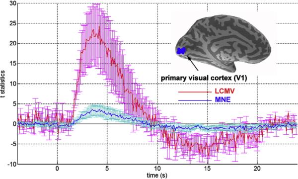
Single subject InI reconstruction time courses and the location of the primary visual cortex (V1) ROI (inset). The time courses show the average (red/dark blue) and the standard deviation (magenta/light blue vertical error bars) of the InI LCMV-dSPM and MNE-dSPM t-values within the V1 ROI.
The time course of the corresponding MNE and LCMV reconstructions are shown in Fig. 5. The LCMV data exhibit clearly superior detection sensitivity, as we observed an approximate five-fold increase in the peak t-statistic in the V1 ROI. However, we observed that within V1 ROI, the baseline variability of the LCMV reconstruction was larger compared to the MNE reconstructions. To further investigate the origin of the higher detection sensitivity associated with the use of LCMV estimation, we plotted the spatial distribution of the baseline variability seen with both the LCMV and MNE inverse operators, as shown in Fig. 6. It is clear that LCMV generally gives higher source variability estimates at the center of the brain. This is physically reasonable since, in this location, there is less spatially overlapping information from the array coil channels and therefore more expected uncertainty in localization. Although MNE results show a similar trend, namely an increased variability of the source estimates at deeper locations, in the V1 ROI the MNE estimate has only 30% baseline variability compared to the LCMV estimate, which can be seen from the baseline t-statistics shown in Fig. 5. Even so, the LCMV reconstruction is associated with a five-fold increase in sensitivity to task-related activity, as evidenced by higher peak t-statistics and higher contrast-to-noise. Taken together, these results support the interpretation that the relative improvement in detection sensitivity in LCMV results from the improved contrast between task and baseline conditions, rather than from suppressed baseline noise. Overall, the increased peak t-statistics and the baseline t-statistic variability in the LCMV reconstructions likely result from the suppression of other source locations by the spatial filter. Indeed, the suppression of other source locations in LCMV may cause difficulties in discriminating two sources close to each other. However, this problem in discriminating nearby sources also exists in the minimum-norm estimates (MNE), since MNE provides spatially blurred reconstructions. Thus, these effects speak to the challenges routinely encountered in distributed source modeling. With better prior knowledge about the number of discrete signal sources, a superior solution might involve utilization of a method similar to the multiple equivalent current dipole (ECD) modeling approach often used with MEG or EEG data, where the solution has a point spread function like a delta function. However, this possibility also leads to questions about the number of sources specified a priori. We suggest that careful consideration of all aspects of signal sources, including the number of expected clusters, their sizes, and their spatial distributions, can allow a principled decision concerning the choice of the best inverse solution employed in order to achieve the optimal reconstruction.
Fig. 6.

The spatial distribution of the standard deviation of the noise estimates from a single subject in LCMV-dSPM and MNE-dSPM in arbitrary units.
LCMV spatial filters are parameterized by a regularization parameter (Eq. (8)). To further evaluate the origin of improved sensitivity in LCMV reconstructions, we parametrically varied the SNR between 0.1 and 100 (Eq. (9)). Since the regularization parameter is inversely proportional to the square of specified SNR, varying SNR allows investigation of the effects of regularization on the LCMV reconstruction. In the V1 ROI time courses corresponding to different SNR values shown in Fig. 7, we observed very similar results for SNR values of 0.1, 3, and 10. Note that even with an exceptionally high SNR value of 100, the time course peak changed less than 10%. In our experience, the SNR in common event-related BOLD fMRI experiments using 6 min of data acquisition and 120 total events ranges from 3 to 15. The high SNR case (SNR = 100) can be regarded as the minimal regularized LCMV reconstruction. Compared to MNE reconstruction, the improved sensitivity observed with LCMV results more from its incorporation of spatial filtering rather than from differing sensitivity to regularization parameters.
Fig. 7.

The time courses of the InI LCMV-dSPM t-values within the V1 ROI from a single subject with specified SNRs of 0.1, 3, 10, and 100.
Group analysis
Strong task-related activity effects can also be easily seen in group average time series. Fig. 8 shows 100 ms duration frames of InI dSPM t-values averaged over 6 participants. The individual frames of this group average show progressively increasing activity starting at 2.4 s after the stimulus onset (critical threshold t>8; uncorrected p-value b 10−4). The signal returns to baseline approximately 6.9 s after stimulus onset.
Fig. 8.

Group average task-related activity. (Top) An inflated left hemisphere cerebral cortex with anatomical orientation (A: anterior; P: posterior; S: superior; I: inferior). Light and dark gray represent gyri and sulci. The calcarine sulcus is labeled. The dashed box indicates the border of the InI LCMV-dSPM single frame time series. (Bottom) Single frames of the InI LCMV-dSPM t-values in visual cortex averaged across five participants shown from the medial aspect of the left hemisphere using an inflated brain surface model. The critical threshold was t>8 (uncorrected p-value<10−4).
The time course of the InI dSPM t-values from the group average are shown in Fig. 9. The shape of this average time series is very similar in character to the individual participant time series shown in Fig. 5, qualitatively demonstrating the between-subject reliability of LCMV InI reconstruction. We observed a reduced variability in the group time course as compared with the individual time courses. Peak task-related activity was found 4.5 s after stimulus onset and a post-stimulus signal undershoot was observed between 10 s and 24 s after stimulus onset. Consistent with the individual participant results, LCMV InI reconstructions show an approximately four-fold increase in detection sensitivity compared to the MNE InI reconstructions (LCMV: 15.9; MNE: 3.4).
Fig. 9.
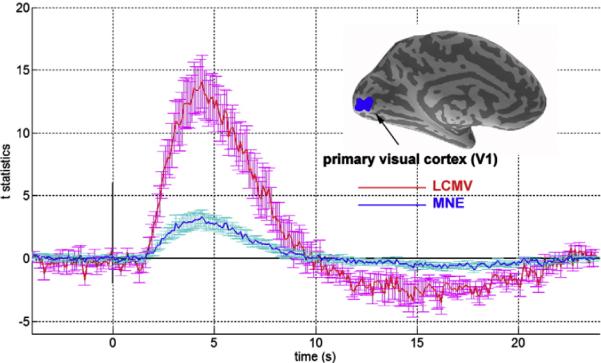
Group average InI reconstruction time courses and the location of the primary visual cortex (V1) ROI (inset). The time courses show the average (red/dark blue) and the standard deviation (magenta/light blue vertical error bars) of the InI LCMV-dSPM and MNE-dSPM t-values within the V1 ROI.
To examine the differences between MNE and LCMV reconstructions across participants, we examined the t-value maxima and the t-value baseline standard deviation in primary visual cortex ROIs from each participant (see Table 2). Generally, LCMV reconstructions were associated with higher peak t-values (average 15.87) compared to MNE reconstructions (average 3.40), reflecting a 4.67-fold advantage. Although the baseline variability of LCMV (average 0.95) was also higher than that of MNE (average 0.34) by 2.79-fold, the relatively larger peak t-values results in a net detection advantage for the LCMV approach.
Table 2.
The t-value maxima and t-value baseline standard deviation in primary visual cortex for MNE and LCMV InI reconstructions of the 6 participants
| Participant | MNE |
LCMV |
||
|---|---|---|---|---|
| Peak t statistics | Baseline t statistics variability | Peak t statistics | Baseline t statistics variability | |
| 1 | 3.45 | 0.32 | 23.67 | 1.20 |
| 2 | 5.47 | 0.24 | 29.11 | 0.68 |
| 3 | 2.06 | 0.43 | 7.04 | 1.42 |
| 4 | 2.79 | 0.29 | 13.50 | 0.74 |
| 5 | 3.87 | 0.41 | 10.37 | 0.70 |
| 6 | 2.78 | 0.34 | 11.54 | 0.94 |
| Average | 3.40 | 0.34 | 15.87 | 0.95 |
On average, LCMV InI estimates were associated with higher peak t-statistics and a higher ratio between the peak t-statistics and the baseline t-statistic variability than were the MNE values.
Discussion
As the brain is a highly dynamic system, accurate estimation of the timing of neural activity is required to fully model the information flow among functionally specialized regions whose aggregate activity underlies perception, cognition and action. Event-related fMRI (Rosen et al., 1998) is a widely utilized neuroimaging method that allows estimation of information processing by measuring the spatial and temporal modulation of the hemodynamic changes associated with changes in neural activity. Event-related experiments have some advantages over block design experiments, which, while allowing high detection sensitivity and fine spatial localization, can only reveal relatively coarse temporal features of task-related activity. In contrast, the superior timing information available with event-related fMRI allows study of both transient and steady state responses, potentially mitigating the bias originating from context or subject expectancy by allowing mixture of various event-types. Event-related fMRI also enables the analysis of data using post-hoc categorization based on the nature of the participant's response (Wagner et al., 1998). In addition, some very successful experimental designs, such as the “odd-ball” experiment, can only be implemented using event-related rather than block designs (Friston, 2007). All the reasons described above encouraged us to explore the feasibility of volumetric InI data acquisition and reconstruction using an event-related fMRI design.
Crude hemodynamic timing information can be estimated by traditional event-related fMRI analysis techniques using deconvolution, which allows temporal resolutions ranging between 2 and 4 s for whole-brain coverage using cubic voxels. This sampling rate is bounded by the timing requirements of multislice EPI acquisition and the associated specific imaging parameters, including number of slices, image matrix size, and receiver bandwidth. In the context of event-related fMRI, single-shot volumetric InI can alleviate the complexities associated with the fact that multislice acquisition is distributed over time. Slice time correction can be implemented either using temporal data interpolation to simulate simultaneous data acquisition or by modeling the relative slice acquisition delays (Friston, 2007). However, temporal data interpolation cannot accurately correct temporally aliased cardiac and respiratory components whose spectra are above the Nyquist sampling frequency of 1/2 TR. Single-shot volumetric acquisition offers direct simultaneous acquisition of data from the entire brain and its use in volumetric InI allows relatively rapid sampling at the cost of moderate reductions in maximum spatial resolution.
The high temporal resolution of volumetric InI also allows estimation of relative task-related timing differences at particular brain locations. Even though BOLD-contrast responses are somewhat sluggish, higher temporal resolution is still desirable for better characterization of the latency and shape of task-related hemodynamic responses (Miezin et al., 2000). The accuracy of relative neural activity onset latency estimates are also directly related to fMRI sampling rates. Limited by a temporal resolution spanning seconds, the traditional EPI multislice acquisition relies heavily on modeling techniques to estimate activity response latency. For example, the latency of BOLD-contrast responses has been estimated from the linear intercept of the signal increase (Menon et al., 1998) or the peak of task-related signal detected using spline interpolation (Huettel and McCarthy, 2001). Alternatively, the ratio of the estimates of the hemodynamic response function and its temporal derivative can also be used to estimate the latency of BOLD-contrast responses (Friston et al., 1998). Different approaches have been suggested to improve the temporal resolution of fMRI, including temporal jittering of stimuli within one TR (Friston, 2007) or using echo-shift pulse sequences (Liu et al., 1993). However, these approaches either require longer time series for stable BOLD-contrast response estimates, or suffer from reduced signal-to-noise ratio. Without a heavy dependence on complicated modeling techniques following image reconstruction, volumetric InI can achieve a direct temporal resolution of 100 ms at SNRs comparable to those currently achieved with multislice EPI.
Single-shot volumetric InI methods can achieve an order-of-magnitude acceleration in hemodynamic response sampling by combining dense head-array coil parallel data acquisition with distributed source modeling. Applying volumetric InI to study task-related visual responses using an event-related design, we found that the method is both sensitive and reliable, as demonstrated in both individual participant and group average results. The InI method described here offers two principal advantages. First, it allows collection of whole-brain volumetric data using single-shot EPI acquisition, while previously it was only possible to obtain one single 2D image at high temporal resolution (20 ms). Volumetric acquisition is more attractive to neuroscientists primarily interested in investigating whole-brain spatiotemporal activity patterns. By sampling the entire brain, volumetric InI can avoid the need for tedious manual slice prescription based on the prior anatomical scans required to identify target brain areas. Second, our approach combines volumetric InI and event-related fMRI design. The volumetric InI acquisition and reconstruction techniques had sufficient sensitivity to reliably detect task-related activity in visual areas with high temporal resolution. Our current experimental design used rather simple stimuli and thus it was difficult to show widely distributed brain activity as is the observed activity was limited by the physiology of regional functional specialization in the visual system. The purpose of this communication is to introduce this novel data acquisition and image reconstruction approach to the neuroimaging community, who may make best use of it to study more complex patterns of spatiotemporal activity. More refined manipulation of the experimental conditions is likely to more fully demonstrate the power of this new tool and we expect to pursue these goals rather soon.
Relationship between LCMV and MNE
The LCMV inverse operator introduced here is closely related to the minimum-norm estimate (MNE) procedure used in our 2D and 3D MR inverse imaging methods (Lin et al., 2006, 2008). For source modeling of MNE and EEG, both LCMV and MNE have been extensively used (Hamalainen et al., 1993) and the equivalence in the mathematical formulation between LCMV and MNE has been proven (Mosher et al., 2003). While both MNE and LCMV need to invert the “data covariance” matrix, the difference between the two is that LCMV derives this data covariance matrix empirically from direct measurements, while MNE indirectly derives the matrix from the forward operator, the noise covariance matrix, and the regularization parameter DMNE = AAH + λ2 C. Thus, while LCMV can be considered as a data-driven method to derive an inverse solution, MNE is a model-driven approach. It is notable that LCMV also has a normalization term in the denominator of the spatial filter in order to ensure a unit gain at each source location. Compared to MNE, this normalization procedure also helps to achieve more homogenous spatial resolution and higher localization accuracy, as demonstrated in Figs. 1 and 2.
The dependence of LCMV on the regularization parameter
The MNE inverse requires a regularization parameter during the derivation of the inverse operator. This is because the matrix product AAH may not have a full rank due to similar lead field patterns from different channels of the coil array. A rank-deficient product of AAH prohibits the construction of a MNE inverse operator since a required matrix inversion does not exist. To address this issue, a fully ranked noise covariance matrix is introduced as a remedy for the rank deficiency. The dependency on the noise covariance is balanced between the amplitude (SNR) of the measurement and the “size” of AAH:
In LCMV estimation, we do not require a regularization parameter if we provide a full rank data covariance matrix. With long enough measurements, a full rank data covariance can usually be calculated directly. The rule-of-thumb suggested is that the “number of measurements should be at least three times as long as the number of sensors” (Van Veen et al., 1997). However, a full rank noise covariance can still be added to improve the conditioning of the data matrix in LCMV inverse if desired as described in Eq. (9).
Alternatively, a regularization parameter can be estimated by L-curve (Hansen, 1998) or generalized-cross-validation (Golub et al., 1979). However, LCMV estimation is not as sensitive to regularization as MNE. Indeed, in our simulations (Figs. 1, 2,and Table 1) we observed that both spatial resolution and localization accuracy are marginally modulated by the imposed regularization parameter or the specified SNR. This argument is further supported by the observation of similar BOLD time courses in V1 from empirical data reconstructed using different regularization parameters.
Correlated sources
One major challenge of the LCMV inverse technique is that LCMV estimation may not be able to detect highly correlated signal sources. This is the consequence of the inverse operator derivation. Specifically, the inverse of the data covariance matrix implies the structure of the “partial correlation coefficient matrix” between different channels (Dempster, 1972). A pair (channel i and j) of highly synchronized sources will attenuate each other in the inverse of the data covariance matrix and thus contribute minimally to the collection of reconstructed sources. However, a high correlation between sources is quite rare under physiological conditions. In fact, LCMV has been previously applied to imaging of coherent neuronal oscillations (Gross et al., 2001). Other simulation studies also support the use of LCMV in the presence of intermediate source correlation (Sekihara et al., 2002). As all of these results were obtained using MEG and EEG signals, which are physiologically quite different from fMRI hemodynamic BOLD-contrast responses, we will attempt to investigate the detection sensitivity of LCMV to correlated sources in the near future.
Spatial resolution
InI solves an ill-posed inverse problem in image reconstruction. Namely, the limited spatial resolution from all channels of the coil array may not be able to provide a unique solution for image reconstruction. This deficiency in independent coil information leads to limits in spatial resolution. However, from our empirical results, we can see that volumetric LCMV InI provides reasonable spatial resolution and localization accuracy when compared to MNE. From our simulation studies, we showed that the spatial resolution of LCMV InI varied with both SNR and source location. For SNRs between 1 and 10, LCMV with noise normalization can potentially achieve 1 mm average point spread function and 1 mm localization accuracy. Additional factors, including but not limited to, coil geometry and field strength, also affect the spatial resolution. Further empirical studies and theoretical calculations are required in order to quantify the influence of these factors on spatial resolution.
The spatial resolution in volumetric InI is spatially-varying because the total amount of independent spatial information from the coil array channels varies among the voxels within the field-of-view. In LCMV, two factors contribute to both the aPSF spatial homogeneity and the localization accuracy (Figs. 1 and 2). First, the denominator in the LCMV inverse operator imposes a “normalization” factor to ensure a unit gain from the spatial filter at each source location. Second, the noise normalization procedure further reduces the spatial-varying amplification of the reconstruction when baseline data are used. Both factors work together to minimize the anisotropy of spatial resolution in the InI encoding direction. In volumetric InI, anisotropic spatial resolution effects only appear in the InI encoding dimension (left–right axis in this study), while the other two spatial dimensions (anterior–posterior and superior–inferior axes) still retain isotropic spatial resolution because gradient encoding is used. To improve the spatial resolution, there are two alternatives. First, increasing the number of channels in a coil array can provide more independent spatial information. However, the benefits obtained from increasing channels will reach a plateau determined by electromagnetic theoretical limitations (Ohliger et al., 2003; Wiesinger et al., 2004). In addition, at higher magnetic fields more independent spatial information can be obtained from the same coil array geometry as the consequence of the shorter peak proton resonance wavelength. This implies that higher spatial resolution can be obtained at 7 T, using the existing 32-channel coil array geometry. Second, we can ameliorate the spatial blurring using other inverse reconstruction kernels, as discussed in the following section.
Applying the LCMV spatial filter at a particular location specifically suppresses contributions at all other source locations. This phenomenon is shown in our point spread function analysis (Fig. 1). However, sharpening a filter's spatial resolution can be either beneficial or disadvantageous. For example, in estimation of the spatial resolution of an actual source, which is theoretically impossible to derive due to the ill-posed nature of the computational process, a sharpened point spread function may lead to underestimation of the actual source size. On the other hand, if the actual sources are spatially focal, sharpened point spread functions can provide better estimates of the spatial location and distribution of the sources compared to other inverse solutions employing wider point spread functions. One good example of this dilemma is the observed sharpening of the point spread function when using equivalent current dipole (ECD) modeling with MEG/EEG data. Resembling a delta function, ECD modeling has the most focal point spread function, making it very useful in seizure focus estimation since epileptic events are generally spatially focal. However, when estimating spatially distributed brain activation, such as that underlying cognitive function, ECD may be an inferior choice compared to other distributed source modeling alternatives (Hamalainen et al., 1993). In summary, tuning the point spread function has been one approach to optimize the performance of inverse solutions, and this rationale has been proposed by Backus and Gilbert in geophysical applications (Backus and Gilbert, 1970). However, caution must still be taken when using inverse solutions with sharpened point spread functions, including, but not limited to, LCMV spatial filters, when prior knowledge about the true source spatial extent may be imperfect.
Spatial distortion
In this study we employed single-shot volumetric InI acquisition with an EPI readout. Thus, the reconstructed projection image contains the expected EPI artifacts, including intravoxel signal loss due to spatially inhomogeneous susceptibility distribution and geometrical distortion along the phase encoding direction due to the intrinsically narrower bandwidth. Correction of these artifacts has been extensively investigated. For example, to mitigate these artifacts, we can use field mapping to estimate the spatial distribution of the off-resonance effects and then use this information to reduce the susceptibility artifacts (Chen et al., 2006; Chen and Wyrwicz, 1999; Zeng and Constable, 2002). It is also possible to use parallel imaging techniques with EPI acquisition methods to limit geometric distortion (Weiger et al., 2002), by systematically skipping multiple integer lines in the continuous sampling of different phase encoding lines and then reconstructing the skipped phase encoding lines using spatial information embedded inside different array channels. Thus, the effective bandwidth in the reconstructed image will be wider and will thereby reduce the spatial distortion. Note that the spatial information from the coil array channels is in an orthogonal direction between EPI phase encoding (anterior–posterior axis) and InI encoding (left–right axis) directions. Although the implementation of this line skipping approach will not reduce the available spatial information in the InI reconstructions, concomitant SNR loss is a price that must be paid for fewer data samples and changes in the parallel MRI reconstruction geometrical factor (g-factor).
Future development
In MEG or EEG source localization, one solution to the ill-posed inverse problem was to add mathematical constraints to limit the “power” of the estimated source in order to obtain a spatially distributed source model. This class of approaches has included the use of L-1 and L-2 norm constraints, which respectively require the source models to have a minimal L-1 and L-2 norms among all possible configurations of sources satisfying the forward solution. The resultant source models were called minimum-current estimates (MCE) (Matsuura and Okabe, 1995; Uutela et al., 1999) and minimum-norm estimate (MNE). MNE has a computational advantage since an analytic solution can be derived, while MCE requires more complicated linear programming techniques to obtain a focal source estimates compared to MNE. In experimental conditions where focal sources are expected, it may be possible to use MCE to reconstruct volumetric InI data in order to further improve spatial resolving power.
Even though volumetric InI allows dramatic increases in sampling rates, it is still constrained by the need to use the optimal TE for detection of BOLD-contrast effects (approximately 30 ms at 3 T). At higher field strengths, such as 7 T, the optimal TE for detecting BOLD-contrast changes is approximately 20 ms, allowing further acceleration of volumetric InI data acquisition, possibly to 50 ms for the whole-brain sampling. In addition, there are two potential approaches to mitigate the temporal resolution limitations. First, we may use different contrast mechanisms, such as steady state free precession (SSFP), where the TE is usually less than 5 ms (Miller et al., 2003, 2006). Second, we may use an echo-shifting technique to reduce the TR (Golay et al., 2000; Liu et al., 1993), as demonstrated in our previous 2D InI study (Lin et al., 2006). Both alternatives are capable of reducing the sampling time to around 20 ms. The resulting higher temporal resolution may allow study of relative cortical activity timing on an extraordinarily fine time scale, thereby facilitating study of the complex interactions among regionally specialized neural subsystems responsible for the mediation of complex behavior.
MRI acoustic noise is generated by the induced Lorentz force interacting with the current passing through the gradient coil perpendicular to the main field B0. The Lorentz force acting on the gradient coil causes vibration similar to a loudspeaker (Schmitt et al., 1998). This acoustic noise is particularly prominent in EPI, where fast oscillatory gradients are used to accelerate k-space traversal. To mitigate this acoustic noise, a sparse sampling method has been proposed (Edmister et al., 1999; Hall et al., 1999; Schwarzbauer et al., 2006; Talavage et al., 1999) at the cost of a lowered data collection efficiency. Alternatively, the gradient waveforms have been smoothed to suppress the noise level (Hennel et al., 1999). A BURST sequence (Jakob et al., 1997, 1998) using 180-degree RF pulses has also been used to collect trains of echoes with a constant gradient. Due to minimal gradient encoding, InI can provide an alternative approach to reduce acoustic scanner noise by minimal phase encoding and/or frequency encoding. This is especially important for investigations of the human auditory system using fMRI.
Acknowledgments
This work was supported by National Institutes of Health Grants by R01DA14178, R01HD040712, R01NS037462, P41 RR14075, R01EB006847, RO1EB000790, R21EB007298, and the Mental Illness and Neuroscience Discovery Institute (MIND), NSC 96-2320-B-002-085 (National Science Council, Taiwan), and NHRI-EX97-9715EC (National Health Research Institute, Taiwan).
References
- Backus GE, Gilbert F. Uniqueness in the inversion of inaccurate gross Earth data. Philos. Trans. R. Soc. Lond., A. 1970;1172:123–192. [Google Scholar]
- Barnes GR, Hillebrand A. Statistical flattening of MEG beamformer images. Hum. Brain Mapp. 2003;18:1–12. doi: 10.1002/hbm.10072. [DOI] [PMC free article] [PubMed] [Google Scholar]
- Belliveau JW, Rosen BR, Kantor HL, Rzedzian RR, Kennedy DN, McKinstry RC, Vevea JM, Cohen MS, Pykett IL, Brady TJ. Functional cerebral imaging by susceptibility-contrast NMR. Magn. Reson. Med. 1990;14:538–546. doi: 10.1002/mrm.1910140311. [DOI] [PubMed] [Google Scholar]
- Belliveau JW, Kennedy DN, Jr., McKinstry RC, Buchbinder BR, Weisskoff RM, Cohen MS, Vevea JM, Brady TJ, Rosen BR. Functional mapping of the human visual cortex by magnetic resonance imaging. Science. 1991;254:716–719. doi: 10.1126/science.1948051. [DOI] [PubMed] [Google Scholar]
- Blum MJ, Braun M, Rosenfeld D. Fast magnetic resonance imaging using spiral trajectories. Australas Phys. Eng. Sci. Med. 1987;10:79–87. [PubMed] [Google Scholar]
- Brainard DH. The Psychophysics Toolbox. Spat. Vis. 1997;10:433–436. [PubMed] [Google Scholar]
- Chau W, Herdman AT, Picton TW. Detection of power changes between conditions using split-half resampling of synthetic aperture magnetometry data. Neurol. Clin. Neurophysiol. 2004;2004:24. [PubMed] [Google Scholar]
- Chen NK, Wyrwicz AM. Correction for EPI distortions using multi-echo gradient-echo imaging. Magn. Reson. Med. 1999;41:1206–1213. doi: 10.1002/(sici)1522-2594(199906)41:6<1206::aid-mrm17>3.0.co;2-l. [DOI] [PubMed] [Google Scholar]
- Chen NK, Oshio K, Panych LP. Application of k-space energy spectrum analysis to susceptibility field mapping and distortion correction in gradient-echo EPI. Neuroimage. 2006;31:609–622. doi: 10.1016/j.neuroimage.2005.12.022. [DOI] [PubMed] [Google Scholar]
- Dale AM. Optimal experimental design for event-related fMRI. Hum. Brain Mapp. 1999;8:109–114. doi: 10.1002/(SICI)1097-0193(1999)8:2/3<109::AID-HBM7>3.0.CO;2-W. [DOI] [PMC free article] [PubMed] [Google Scholar]
- Dale AM, Fischl B, Sereno MI. Cortical surface-based analysis: I. Segmentation and surface reconstruction. Neuroimage. 1999;9:179–194. doi: 10.1006/nimg.1998.0395. [DOI] [PubMed] [Google Scholar]
- Dale AM, Liu AK, Fischl BR, Buckner RL, Belliveau JW, Lewine JD, Halgren E. Dynamic statistical parametric mapping: combining fMRI and MEG for high-resolution imaging of cortical activity. Neuron. 2000;26:55–67. doi: 10.1016/s0896-6273(00)81138-1. [DOI] [PubMed] [Google Scholar]
- Dempster AP. Covariance selection. Biometrics. 1972;28:157–175. [Google Scholar]
- Edmister WB, Talavage TM, Ledden PJ, Weisskoff RM. Improved auditory cortex imaging using clustered volume acquisitions. Hum. Brain Mapp. 1999;7:89–97. doi: 10.1002/(SICI)1097-0193(1999)7:2<89::AID-HBM2>3.0.CO;2-N. [DOI] [PMC free article] [PubMed] [Google Scholar]
- Fischl B, Sereno MI, Dale AM. Cortical surface-based analysis. II: inflation, flattening, and a surface-based coordinate system. Neuroimage. 1999;9:195–207. doi: 10.1006/nimg.1998.0396. [DOI] [PubMed] [Google Scholar]
- Fischl B, Liu A, Dale AM. Automated manifold surgery: constructing geometrically accurate and topologically correct models of the human cerebral cortex. IEEE Trans. Med. Imaging. 2001;20:70–80. doi: 10.1109/42.906426. [DOI] [PubMed] [Google Scholar]
- Friston KJ. Statistical Parametric Mapping: The Analysis of Functional Brain Images. 1st ed. Elsevier/Academic Press; Amsterdam: Boston: 2007. [Google Scholar]
- Friston KJ, Fletcher P, Josephs O, Holmes A, Rugg MD, Turner R. Event-related fMRI: characterizing differential responses. Neuroimage. 1998;7:30–40. doi: 10.1006/nimg.1997.0306. [DOI] [PubMed] [Google Scholar]
- Gaetz WC, Cheyne DO. Localization of human somatosensory cortex using spatially filtered magnetoencephalography. Neurosci. Lett. 2003;340:161–164. doi: 10.1016/s0304-3940(03)00108-3. [DOI] [PubMed] [Google Scholar]
- Golay X, Pruessmann KP, Weiger M, Crelier GR, Folkers PJ, Kollias SS, Boesiger P. PRESTO-SENSE: an ultrafast whole-brain fMRI technique. Magn. Reson. Med. 2000;43:779–786. doi: 10.1002/1522-2594(200006)43:6<779::aid-mrm1>3.0.co;2-4. [DOI] [PubMed] [Google Scholar]
- Golub GH, Heath MT, Wahba G. Generalized cross-validation as a method of choosing a good ridge parameter. Technometrics. 1979;21:215–223. [Google Scholar]
- Gross J, Kujala J, Hamalainen M, Timmermann L, Schnitzler A, Salmelin R. Dynamic imaging of coherent sources: studying neural interactions in the human brain. Proc. Natl. Acad. Sci. U. S. A. 2001;98:694–699. doi: 10.1073/pnas.98.2.694. [DOI] [PMC free article] [PubMed] [Google Scholar]
- Hall DA, Haggard MP, Akeroyd MA, Palmer AR, Summerfield AQ, Elliott MR, Gurney EM, Bowtell RW. “Sparse” temporal sampling in auditory fMRI. Hum. Brain Mapp. 1999;7:213–223. doi: 10.1002/(SICI)1097-0193(1999)7:3<213::AID-HBM5>3.0.CO;2-N. [DOI] [PMC free article] [PubMed] [Google Scholar]
- Hamalainen M, Hari R, Ilmoniemi R, Knuutila J, Lounasmaa O. Magnetoencephalography-theory, instrumentation, and application to noninvasive studies of the working human brain. Rev. Mod. Phys. 1993;65:413–497. [Google Scholar]
- Hansen PC. Rank-deficient and Discrete Ill-posed Problems: Numerical Aspects of Linear Inversion. SIAM; Philadelphia: 1998. [Google Scholar]
- Hennel F, Girard F, Loenneker T. “Silent” MRI with soft gradient pulses. Magn. Reson. Med. 1999;42:6–10. doi: 10.1002/(sici)1522-2594(199907)42:1<6::aid-mrm2>3.0.co;2-d. [DOI] [PubMed] [Google Scholar]
- Hennig J, Zhong K, Speck O. MR-Encephalography: fast multi-channel monitoring of brain physiology with magnetic resonance. Neuroimage. 2007;34:212–219. doi: 10.1016/j.neuroimage.2006.08.036. [DOI] [PubMed] [Google Scholar]
- Hu X. On the “keyhole” technique. J. Magn. Reson. Imaging. 1994;4:231. doi: 10.1002/jmri.1880040223. [DOI] [PubMed] [Google Scholar]
- Huettel SA, McCarthy G. Regional differences in the refractory period of the hemodynamic response: an event-related fMRI study. Neuroimage. 2001;14:967–976. doi: 10.1006/nimg.2001.0900. [DOI] [PubMed] [Google Scholar]
- Jakob PM, Griswold MA, Lovblad KO, Chen Q, Edelman RR. Half-Fourier BURST imaging on a clinical scanner. Magn. Reson. Med. 1997;38:534–540. doi: 10.1002/mrm.1910380405. [DOI] [PubMed] [Google Scholar]
- Jakob PM, Schlaug G, Griswold M, Lovblad KO, Thomas R, Ives JR, Matheson JK, Edelman RR. Functional burst imaging. Magn. Reson. Med. 1998;40:614–621. doi: 10.1002/mrm.1910400414. [DOI] [PubMed] [Google Scholar]
- Jones RA, Haraldseth O, Muller TB, Rinck PA, Oksendal AN. K-space substitution: a novel dynamic imaging technique. Magn. Reson. Med. 1993;29:830–834. doi: 10.1002/mrm.1910290618. [DOI] [PubMed] [Google Scholar]
- Kwong KK, Belliveau JW, Chesler DA, Goldberg IE, Weisskoff RM, Poncelet BP, Kennedy DN, Hoppel BE, Cohen MS, Turner R, Cheng H, Brady TJ, Rosen BR. Dynamic magnetic resonance imaging of human brain activity during primary sensory stimulation. Proc. Natl. Acad. Sci. U. S. A. 1992;89:5675–5679. doi: 10.1073/pnas.89.12.5675. [DOI] [PMC free article] [PubMed] [Google Scholar]
- Lin FH, Kwong KK, Belliveau JW, Wald LL. Parallel imaging reconstruction using automatic regularization. Magn. Reson. Med. 2004;51:559–567. doi: 10.1002/mrm.10718. [DOI] [PubMed] [Google Scholar]
- Lin FH, Huang TY, Chen NK, Wang FN, Stufflebeam SM, Belliveau JW, Wald LL, Kwong KK. Functional MRI using regularized parallel imaging acquisition. Magn. Reson. Med. 2005a;54:343–353. doi: 10.1002/mrm.20555. [DOI] [PMC free article] [PubMed] [Google Scholar]
- Lin FH, Huang TY, Chen NK, Wang FN, Stufflebeam SM, Belliveau JW, Wald LL, Kwong KK. Functional MRI using regularized parallel imaging acquisition. Magn. Reson. Med. 2005b;54:343–353. doi: 10.1002/mrm.20555. [DOI] [PMC free article] [PubMed] [Google Scholar]
- Lin FH, Wald LL, Ahlfors SP, Hamalainen MS, Kwong KK, Belliveau JW. Dynamic magnetic resonance inverse imaging of human brain function. Magn. Reson. Med. 2006;56:787–802. doi: 10.1002/mrm.20997. [DOI] [PubMed] [Google Scholar]
- Lin FH, Witzel T, Mandeville JB, Polimeni JR, Zeffiro TA, Greve DN, Wiggins G, Wald LL, Belliveau JW. Event-related single-shot volumetric functional magnetic resonance inverse imaging of visual processing. NeuroImage. 2008;42(1):230–247. doi: 10.1016/j.neuroimage.2008.04.179. [DOI] [PMC free article] [PubMed] [Google Scholar]
- Liu AK, Belliveau JW, Dale AM. Spatiotemporal imaging of human brain activity using functional MRI constrained magnetoencephalography data: Monte Carlo simulations. Proc. Natl. Acad. Sci. U. S. A. 1998;95:8945–8950. doi: 10.1073/pnas.95.15.8945. [DOI] [PMC free article] [PubMed] [Google Scholar]
- Liu AK, Dale AM, Belliveau JW. Monte Carlo simulation studies of EEG and MEG localization accuracy. Hum. Brain Mapp. 2002;16:47–62. doi: 10.1002/hbm.10024. [DOI] [PMC free article] [PubMed] [Google Scholar]
- Liu G, Sobering G, Duyn J, Moonen CT. A functional MRI technique combining principles of echo-shifting with a train of observations (PRESTO) Magn. Reson. Med. 1993;30:764–768. doi: 10.1002/mrm.1910300617. [DOI] [PubMed] [Google Scholar]
- Mansfield P. Multi-planar image formation using NMR spin echos. J. Physics. 1977;C10:L55–L58. [Google Scholar]
- Matsuura K, Okabe Y. Selective minimum-norm solution of the biomagnetic inverse problem. IEEE Trans. Biomed. Eng. 1995;42:608–615. doi: 10.1109/10.387200. [DOI] [PubMed] [Google Scholar]
- McDougall MP, Wright SM. 64-channel array coil for single echo acquisition magnetic resonance imaging. Magn. Reson. Med. 2005;54:386–392. doi: 10.1002/mrm.20568. [DOI] [PubMed] [Google Scholar]
- McGibney G, Smith MR, Nichols ST, Crawley A. Quantitative evaluation of several partial Fourier reconstruction algorithms used in MRI. Magn. Reson. Med. 1993;30:51–59. doi: 10.1002/mrm.1910300109. [DOI] [PubMed] [Google Scholar]
- Menon RS, Luknowsky DC, Gati JS. Mental chronometry using latency-resolved functional MRI. Proc. Natl. Acad. Sci. U. S. A. 1998;95:10902–10907. doi: 10.1073/pnas.95.18.10902. [DOI] [PMC free article] [PubMed] [Google Scholar]
- Miezin FM, Maccotta L, Ollinger JM, Petersen SE, Buckner RL. Characterizing the hemodynamic response: effects of presentation rate, sampling procedure, and the possibility of ordering brain activity based on relative timing. Neuroimage. 2000;11:735–759. doi: 10.1006/nimg.2000.0568. [DOI] [PubMed] [Google Scholar]
- Miller KL, Hargreaves BA, Lee J, Ress D, deCharms RC, Pauly JM. Functional brain imaging using a blood oxygenation sensitive steady state. Magn. Reson. Med. 2003;50:675–683. doi: 10.1002/mrm.10602. [DOI] [PubMed] [Google Scholar]
- Miller KL, Smith SM, Jezzard P, Pauly JM. High-resolution FMRI at 1.5 T using balanced SSFP. Magn. Reson. Med. 2006;55:161–170. doi: 10.1002/mrm.20753. [DOI] [PubMed] [Google Scholar]
- Mistretta CA, Wieben O, Velikina J, Block W, Perry J, Wu Y, Johnson K, Wu Y. Highly constrained backprojection for time-resolved MRI. Magn. Reson. Med. 2006;55:30–40. doi: 10.1002/mrm.20772. [DOI] [PMC free article] [PubMed] [Google Scholar]
- Mosher JC, Baillet S, Leahy RM. Equivalence of linear approaches in biomagnetic inverse solutions. 2003 IEEE workshop on statistical signal processing; IEEE, St. Louis, Missouri. 2003. pp. 294–297. [Google Scholar]
- Ogawa S, Lee TM, Kay AR, Tank DW. Brain magnetic resonance imaging with contrast dependent on blood oxygenation. Proc. Natl. Acad. Sci. U. S. A. 1990;87:9868–9872. doi: 10.1073/pnas.87.24.9868. [DOI] [PMC free article] [PubMed] [Google Scholar]
- Ohliger MA, Grant AK, Sodickson DK. Ultimate intrinsic signal-to-noise ratio for parallel MRI: electromagnetic field considerations. Magn. Reson. Med. 2003;50:1018–1030. doi: 10.1002/mrm.10597. [DOI] [PubMed] [Google Scholar]
- Pelli DG. The VideoToolbox software for visual psychophysics: transforming numbers into movies. Spat. Vis. 1997;10:437–442. [PubMed] [Google Scholar]
- Preibisch C, Pilatus U, Bunke J, Hoogenraad F, Zanella F, Lanfermann H. Functional MRI using sensitivity-encoded echo planar imaging (SENSE-EPI) Neuroimage. 2003;19:412–421. doi: 10.1016/s1053-8119(03)00080-6. [DOI] [PubMed] [Google Scholar]
- Pruessmann KP, Weiger M, Scheidegger MB, Boesiger P. SENSE: sensitivity encoding for fast MRI. Magn. Reson. Med. 1999;42:952–962. [PubMed] [Google Scholar]
- Robinson SE, Vrba J. Functional Neuroimaging by Synthetic Aperture Magnetometry (SAM) Tohoku University Press; Sendai: 1999. [Google Scholar]
- Rosen BR, Buckner RL, Dale AM. Event-related functional MRI: past, present, and future. Proc. Natl. Acad. Sci. U. S. A. 1998;95:773–780. doi: 10.1073/pnas.95.3.773. [DOI] [PMC free article] [PubMed] [Google Scholar]
- Schmidt CF, Degonda N, Luechinger R, Henke K, Boesiger P. Sensitivity-encoded (SENSE) echo planar fMRI at 3 T in the medial temporal lobe. Neuroimage. 2005;25:625–641. doi: 10.1016/j.neuroimage.2004.12.002. [DOI] [PubMed] [Google Scholar]
- Schmitt F, Stehling MK, Turner R, Bandettini PA. Echo-Planar Imaging: Theory, Technique, and Application. Springer; Berlin: 1998. [Google Scholar]
- Schwarzbauer C, Davis MH, Rodd JM, Johnsrude I. Interleaved silent steady state (ISSS) imaging: a new sparse imaging method applied to auditory fMRI. Neuroimage. 2006;29:774–782. doi: 10.1016/j.neuroimage.2005.08.025. [DOI] [PubMed] [Google Scholar]
- Sekihara K, Nagarajan SS, Poeppel D, Marantz A, Miyashita Y. Reconstructing spatio-temporal activities of neural sources using an MEG vector beamformer technique. IEEE Trans. Biomed. Eng. 2001;48:760–771. doi: 10.1109/10.930901. [DOI] [PubMed] [Google Scholar]
- Sekihara K, Nagarajan SS, Poeppel D, Marantz A. Performance of an MEG adaptive-beamformer technique in the presence of correlated neural activities: effects on signal intensity and time-course estimates. IEEE Trans. Biomed. Eng. 2002;49:1534–1546. doi: 10.1109/tbme.2002.805485. [DOI] [PubMed] [Google Scholar]
- Sodickson DK, Manning WJ. Simultaneous acquisition of spatial harmonics (SMASH): fast imaging with radiofrequency coil arrays. Magn. Reson. Med. 1997;38:591–603. doi: 10.1002/mrm.1910380414. [DOI] [PubMed] [Google Scholar]
- Talavage TM, Edmister WB, Ledden PJ, Weisskoff RM. Quantitative assessment of auditory cortex responses induced by imager acoustic noise. Hum. Brain Mapp. 1999;7:79–88. doi: 10.1002/(SICI)1097-0193(1999)7:2<79::AID-HBM1>3.0.CO;2-R. [DOI] [PMC free article] [PubMed] [Google Scholar]
- Taniguchi M, Kato A, Fujita N, Hirata M, Tanaka H, Kihara T, Ninomiya H, Hirabuki N, Nakamura H, Robinson SE, Cheyne D, Yoshimine T. Movement-related desynchronization of the cerebral cortex studied with spatially filtered magnetoencephalography. Neuroimage. 2000;12:298–306. doi: 10.1006/nimg.2000.0611. [DOI] [PubMed] [Google Scholar]
- Tsao J, Behnia B, Webb AG. Unifying linear prior-information-driven methods for accelerated image acquisition. Magn. Reson. Med. 2001;46:652–660. doi: 10.1002/mrm.1242. [DOI] [PubMed] [Google Scholar]
- Uutela K, Hamalainen M, Somersalo E. Visualization of magnetoencephalographic data using minimum current estimates. Neuroimage. 1999;10:173–180. doi: 10.1006/nimg.1999.0454. [DOI] [PubMed] [Google Scholar]
- van Vaals JJ, Brummer ME, Dixon WT, Tuithof HH, Engels H, Nelson RC, Gerety BM, Chezmar JL, den Boer JA. “Keyhole” method for accelerating imaging of contrast agent uptake. J. Magn. Reson. Imaging. 1993;3:671–675. doi: 10.1002/jmri.1880030419. [DOI] [PubMed] [Google Scholar]
- Van Veen BD, Buckley K. Beamforming: a versatile approach to spatial filtering. IEEE ASSP Magazine. 1988;5:4–24. [Google Scholar]
- Van Veen BD, van Drongelen W, Yuchtman M, Suzuki A. Localization of brain electrical activity via linearly constrained minimum variance spatial filtering. IEEE Trans. Biomed. Eng. 1997;44:867–880. doi: 10.1109/10.623056. [DOI] [PubMed] [Google Scholar]
- Wagner AD, Schacter DL, Rotte M, Koutstaal W, Maril A, Dale AM, Rosen BR, Buckner RL. Building memories: remembering and forgetting of verbal experiences as predicted by brain activity. Science. 1998;281:1188–1191. doi: 10.1126/science.281.5380.1188. [DOI] [PubMed] [Google Scholar]
- Weiger M, Pruessmann KP, Osterbauer R, Bornert P, Boesiger P, Jezzard P. Sensitivity-encoded single-shot spiral imaging for reduced susceptibility artifacts in BOLD fMRI. Magn. Reson. Med. 2002;48:860–866. doi: 10.1002/mrm.10286. [DOI] [PubMed] [Google Scholar]
- Wiesinger F, Boesiger P, Pruessmann KP. Electrodynamics and ultimate SNR in parallel MR imaging. Magn. Reson. Med. 2004;52:376–390. doi: 10.1002/mrm.20183. [DOI] [PubMed] [Google Scholar]
- Wiggins GC, Triantafyllou C, Potthast A, Reykowski A, Nittka M, Wald LL. 32-channel 3 Tesla receive-only phased-array head coil with soccer-ball element geometry. Magn. Reson. Med. 2006;56:216–223. doi: 10.1002/mrm.20925. [DOI] [PubMed] [Google Scholar]
- Zeng H, Constable RT. Image distortion correction in EPI: comparison of field mapping with point spread function mapping. Magn. Reson. Med. 2002;48:137–146. doi: 10.1002/mrm.10200. [DOI] [PubMed] [Google Scholar]