Comparing costs associated with risk stratification rules for t-year survival

Abstract

Accurate risk prediction is an important step in developing optimal strategies for disease prevention and treatment. Based on the predicted risks, patients can be stratified to different risk categories where each category corresponds to a particular clinical intervention. Incorrect or suboptimal interventions are likely to result in unnecessary financial and medical consequences. It is thus essential to account for the costs associated with the clinical interventions when developing and evaluating risk stratification (RS) rules for clinical use. In this article, we propose to quantify the value of an RS rule based on the total expected cost attributed to incorrect assignment of risk groups due to the rule. We have established the relationship between cost parameters and optimal threshold values used in the stratification rule that minimizes the total expected cost over the entire population of interest. Statistical inference procedures are developed for evaluating and comparing given RS rules and examined through simulation studies. The proposed procedures are illustrated with an example from the Cardiovascular Health Study.

1. INTRODUCTION

Accurate risk assessment and disease prognosis are essential in health care. To improve disease prevention and management, risk stratification (RS) rules are often developed to assign subjects into different risk groups where each group corresponds a particular intervention. For example, a commonly used RS rule in cardiovascular disease prevention stratifies patients into low, intermediate, and high risk groups. Patients are typically recommended to receive antihypertensive therapy if in the intermediate risk group and receive statin if in the high risk group. In studies designed to develop RS rules, measurements of risk factors are often ascertained at baseline and patients are followed over time for the occurrence of a certain clinical event. Since the risk of experiencing such an event may change over time, one must incorporate the time domain when constructing RS rules. For example, cardiovascular RS rules are often based on the risk of experiencing a cardiovascular event within 10 years since the measurement of the risk factors. In this paper, we are interested in stratification rules for the risk of experiencing an event within t years since marker measurement. Throughout, we use the terms “cases” and “controls” to denote subjects who will and will not experience an event within t years, respectively, if the RS of interest has not been employed. The potential disease status may be changed after patients receive RS-guided intervention.

When developing and evaluating RS rules, it is crucial to understand the potential clinical and financial costs associated with assigning patients into incorrect risk groups and thus receiving suboptimal interventions. Unnecessary medication costs arise when controls are incorrectly assigned to high risk groups. Assigning cases to the low-risk category may lead to costs of life-years lost, productivity, and the subsequent medication. This signifies the importance of precise risk prediction and rigorous evaluation of RS rules prior to their wide spread use in clinical practice.

In practice, RS rules are often derived from risk prediction models with a panel of markers. Based on the predicted risk from the model, future subjects are assigned to different risk categories to receive the corresponding intervention. There are 3 important steps in developing an effective RS rule: (1) constructing a regression model predictive to the clinical response of interest (2) determining the appropriate risk category corresponding to specific intervention, and (3) evaluating the resulting RS rule in an objective and transparent way. While most of statistical methodological research focuses on the step of empirical model building, the clear answer to latter 2 steps remains elusive. When evaluating the performance of risk prediction models, measures of accuracy based on the discrimination and calibration have been considered (Gail and Pfeiffer, 2005), (Cook, 2007). Discrimination measures the ability of the risk prediction model in discriminating cases from controls. Calibration measures how well the predicted risk approximates the true conditional risk given the marker measurements. However, neither of these 2 types of measures are appropriate for evaluating the performance of RS. One of the most commonly used discrimination measure is the receiver operating characteristic (ROC) curve (Pepe, 2003). Since the ROC curve is scale invariant, a monotone transformation of predicted risks does not affect the discriminatory accuracy but could lead to dramatic changes in the assignment of risk groups. Calibration measures such as the Hosmer–Lemeshow goodness of fit statistic are also inadequate because a perfectly calibrated model may have poor performance in RS if the available markers have little power in predicting the outcome. To comprehensively assess a risk model, Pepe and others (2008) advocated the use of a predictiveness curve in conjunction with discriminatory measures. However, such an approach could not be directly applied to evaluate the performance of RS-guided intervention. In the context of evaluating the incremental value of a new marker for risk reclassification, Pencina and others (2008) proposed to measure the net reclassification improvement (NRI) based on the proportion of subjects reclassified into higher- or lower-risk categories. The NRI can be used to compare RS rules but not to evaluate a single RS rule. Furthermore, the NRI does not account for the differential costs associated with different types of incorrect assignment.

The ultimate value of an RS rule can be represented as the extra total cost/benefit if the RS-guided intervention applied to the target population. Therefore, to effectively construct and evaluate an RS rule, one should have information on the financial and medical costs/benefits associated with the interventions. Therefore, an ideal data set to evaluate the RS rule would consist of patients whose intervention status is known. With such a data set along with the cost/benefit information on the interventions, one may comprehensively evaluate an RS rule based on the expected cost associated with incorrect assignment of risk groups. In this paper, we propose a unified framework to determine the optimal risk categorization and quantify the value of the corresponding RS rule based on the expected costs when the cost parameters are assumed to be given. As a simple example, patients may be stratified into low or high risk groups where low-risk patients would be managed without intervention and high-risk patients would receive a treatment. Two types of costs may arise from such a stratification: the unnecessary intervention for controls, denoted by C₀; and the cost of not receiving treatment for cases, denoted by C₁. When evaluating an RS rule that differentiates the high- and low-risk patients, it is important to account for the trade-off between these 2 types of costs (Cantor and others, 1999), (Obuchowski, 2003) and develop an RS rule with a cutoff value that optimizes the trade-off between these costs. In Section 2, we discuss the relationship between costs and optimal threshold values of an RS rules based on a single marker. Procedures for comparing multiple RS rules are also discussed. These procedures are generalized to the setting where multiple risk factors are available for RS in Section 3. The proposed methods are illustrated in Section 3 with a data set from the Cardiovascular Health Study (CHS) and simulation studies. Some remarks are given in Section 5.

2. OPTIMAL RS RULES WITH A SINGLE MARKER

Let T denote the time to developing a clinical event and suppose interest lies in predicting the risk of failing by time t, that is, Y = I(T ≤ t). We first consider the setting where a single continuous marker Z is used to construct RS rules. Z could be a biomarker or a composite risk score established in the literature. Without loss of generality, we assume that the goal is to assign subjects into k = 1,…,K increasingly ordered risk categories.

2.1. Optimal threshold values of RS and prespecified costs

Let R(z):( − ∞,∞)→{1,…,K} denote the risk group assignment with marker Z = z based on its predicted risk m(z). A subject would be assigned to a low-risk category if m(z) is close to 0 and to a high-risk category if m(z) is sufficiently larger than 0. The risk threshold values for the optimal RS rule are directly related to the costs associated with incorrect assignment of risk groups. An optimal rule would assign cases to the highest risk category and controls to the lowest category. Let c_1k and c_0k denote the cost associated with assigning cases and controls to the kth risk category, respectively. Then we expect that c₁₁ > c₁₂ > ⋯ > c_1K and c₀₁ < c₀₂ < ⋯ < c_0K. Without loss of generality, we assume that c_1K = c₀₁ = 0. Under this assumption, c_1k essentially represents the additional cost incurred by assigning a case to the kth category as opposed to the highest category; and c_0k represents the additional cost associating with assigning a control to the kth category when compared to the lowest category.

We propose to summarize the performance of R(z) for the subpopulation with marker value Z = z using the expected cost associated with the stratification:

We show in online Appendix A that among all possible stratification rules based on Z, the optimal stratification rule that achieves the lowest expected cost is

where . Here, r_kl is the incremental cost by moving a diseased subject from risk category k to l relative to the incremental cost by moving a disease-free subject from risk category l to k.

For a given set of cost parameters, the optimal RS rule may suggest that not all K categories are necessary. As an example, we show the optimal RS rule for K = 3 in Table 1. When the relative cost r₃₂ ≥ r₁₂, the optimal rule classifies no subject as intermediate risk suggesting that there is no gain of having the intermediate risk category under such a condition. In general for assigning K risk categories, the optimal RS rule will not contain empty cells or unnecessary risk strata if and only if

(2.1)

Table 1.

Optimal stratification rules under various configurations when K = 3. Here, ∅ represents an empty set suggesting that no subject would be assigned to the risk category

Ropt(z)	r32 < r21	r32 ≥ r21
1	μ0(z) ≤ P21	μ0(z) ≤ P31
2	μ0(z)∈(P21,P32]	∅
3	μ0(z) > P32	μ0(z) > P31

Under such an assumption, the optimal RS rule is

(2.2)

(2.3)

which infers that

(2.4)

Equations (2.3) and (2.4) characterize the relationship between optimal threshold values of an RS and the cost parameters.

2.2. The expected cost of an RS rule with optimal threshold values

Suppose the optimal threshold values, p = (p₁,…,p_K)^T, are used to create K increasing risk categories. A subject with predicted risk m(z) will be assigned to the kth risk category if m(z)∈(p_{k − 1},p_k], where 0 = p₀ < p₁ < ⋯ < p_K = 1. The overall performance of such a stratification rule can be evaluated based on the expected cost, where

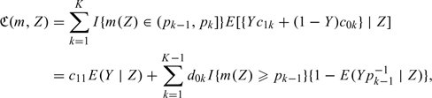where . Utilizing (2.4), we represent in terms of p and c₀ = (c₀₁,…,c_0K)^′. The advantage of this representation is that c_0k is relatively easy to ascertain based on the financial cost of applying the corresponding intervention to a healthy subject if one is willing to ignore the side effects of the intervention. On the contrary, it is generally difficult to determine c_1k, the cost of cases receiving the incorrect intervention. Obviously, the RS with the true conditional risk function μ₀(·), achieves the lowest expected cost among all RS rules based on Z.

Since the commonly used risk threshold values are often derived from a series of careful adjustments based on the empirical results from long-term clinical practice, it is not unreasonable to assume that such threshold values of a well-established RS rule are “optimal” with respect to a set of underlying cost values, which are implicitly accepted by public. Under such an optimality assumption, one may use to evaluate the RS rule. Furthermore, the expected cost function provides a mechanism for comparing RS rules based on different risk scores. For example, if 2 risk scores Z⁽¹⁾ and Z⁽²⁾ are available for RS, one may prefer the risk score Z⁽¹⁾ over Z⁽²⁾ if and Z⁽²⁾ over Z⁽¹⁾, otherwise, where μ_j0(z) = pr(Y = 1∣Z^(j) = z),j = 1,2. When the risk scores involve potentially expensive or invasive markers, one may also incorporate the cost associated with the ascertainment of the risk scores when comparing their performances. Specifically, let C_j be the average cost associated with ascertaining the risk score Z^(j), then the expected costs associated with Z^(j) is . Thus, one may prefer Z⁽¹⁾ over Z⁽²⁾ if .

2.3. Evaluating the optimal RS rules

Let T_i and Z_i denote the event time and marker value for the ith subject, respectively. Due to censoring, for T_i, one observes (X_i,δ_i), where X_i = min(T_i,T_i^cen), δ_i = I(T_i ≤ T_i^cen), and T_i^cen are the follow-up time for the ith subject assumed to be independent of T_i and Z_i with a common G(t) = pr(T^cen ≥ t). Data for analysis consist of n i.i.d. random vectors, {(X_i,δ_i,Z_i),i = 1,…,n}.

Estimating expected cost.

Without censoring, the expected cost associated with a risk score m(z) based on known p and c₀, may be estimated nonparametrically by

where . However, Y_i is not always observable due to censoring. To incorporate censoring, we propose to modify based on the inverse probability weighting (IPW) estimator

(2.5)

where and is the Kaplan–Meier estimator of G(t).

Estimating the conditional risk.

The true conditional risk function μ₀(z) = pr(Y = 1|Z = z) involved in the optimal RS is unknown in general. To estimate μ₀(z) nonparametrically, we consider the use of the local logistic likelihood estimator (Tibshirani and Hastie, 1987) with IPW to account for censoring. Specifically, we estimate μ₀(z) by , where is the solution to the local IPW score equation

(2.6)

where K_h(z) = h ^{− 1}K(z/h), K(·) is a smooth symmetric density function and h is the bandwidth with h→0 and nh²→∞ as n→∞. In practice, the bandwidth h for estimating the conditional risk function may be selected via 𝒦-fold cross validation.

Interval estimation procedures for .

To obtain interval estimates for , we show in online Appendix B that is consistent for . Furthermore, under mild regularity conditions, converges in distribution to a zero-mean normal with variance σ². A 95% confidence interval for may be obtained as , where is a consistent estimator of σ obtained by replacing all the theoretical quantities in σ by their empirical counterparts.

When there are multiple markers available, one may compare the performance in RS based on the difference between the expected costs. For example, when there are 2 risk scores, Z⁽¹⁾ and Z⁽²⁾, one may compare their corresponding RS performances based on , where

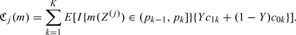may be consistently estimated by , where is the estimated risk function based on Z^(j) and , for j = 1,2. Using similar arguments as given in online Appendix B, one may show that converges in distribution to a zero-mean normal with variance σ_Δ². The confidence intervals can be constructed accordingly.

3. APPROXIMATING OPTIMAL RS RULES BASED ON MULTIPLE MARKERS

3.1. Developing RS rules

When there are a panel of markers, denoted by a column vector Z, available for risk prediction, one may derive RS rules by first ascertaining the conditional risk function, μ₀(Z) = pr(Y = 1∣Z). For the subpopulation with Z = z, the optimal RS rule may be constructed by replacing μ₀(z) in (2.2) with μ₀(z). In general, for any given risk prediction function μ(z) and cost parameters, one may construct an RS rule based on R_μ(Z) = ∑_{k = 1}^KI{μ(Z) ≤ p_k}, where p_k is given in (2.3). The total expected cost associated with such a rule for is ℂ(μ) = E{ℂ(μ,Z)}, where

The true conditional risk function μ₀(·) minimizes the total expected cost ℂ(μ) among all functions of Z. To approximate the optimal RS rule based on available data, one needs to estimate μ₀(Z). When the number of markers is not small, it is implausible to estimate μ₀(Z) nonparametrically. A practical approach is to approximate the conditional risk through regression modeling. For example, one may consider regression models such as the Cox proportional hazards model (Cox, 1972), semiparametric transformation models (Cheng and others, 1995) or time-specific generalized linear models (GLMs) (Zheng and others, 2006; Uno and others, 2007). When the assumed regression model is the true model, one may estimate μ₀(Z) consistently by fitting the regression model.

In practice, simple regression models may fail to hold. As such, the estimated conditional risk function may be a poor approximation to the true conditional risk and thus leads to suboptimal RS rules. Furthermore, inference procedures about the performance of the RS rule may be invalid if such procedures are derived under the assumption of correct model specification. To overcome such difficulties, we propose to employ simple statistical models as “working” models for approximating the true conditional risk and derive procedures for making inference about the performance of RS rules without requiring the fitted model to hold. A wide range of survival models including those mentioned above may be considered as the working model. A simple example is to model the conditional risk function μ₀(Z) via the time-specific GLM,

(3.1)

where g(·) is a prespecified monotone and smooth link function and β is an unknown regression coefficient. Without loss of generality, we assume that the vector Z includes 1 as its first component. Here, both g and β could may vary with time t. Through the working model (3.1), one may approximate the conditional risk for a subject with Z = z as , where is the solution to

(3.2)

Uno and others (2007) showed that is always convergent to β₀, the unique solution to E[Z{Y − g(β^TZ)}] = 0.

Based on the working model (3.1), one may construct RS rule using the risk prediction function g(β₀^TZ). However, if the working model (3.1) fails to be a good approximation to the true model, it is unclear whether such an RS rule is optimal in any sense and may not perform well. To improve the RS, we propose to use β₀^TZ as a scoring system and predict the risk for a subject with Z as μ_β0(Z), where μ_β(Z) = pr(Y = 1∣β^TZ). An optimal RS rule based on μ_β0(Z) may be constructed as in (2.2). Such a rule would be optimal, with respect to ℂ(μ), among all rules based on Z if the working model holds and optimal within rules based on the linear risk score β₀^TZ if the working model fails to hold. Compared with g(β₀^TZ⁰), it is straightforward to show that

and we expect that RS rules based on μ_β(Z) will have lower expected cost compared to that based on g(β₀^TZ).

For any given z, a consistent estimate of μ_β0(z) may be obtained as , where is the nonparametric local likelihood estimator similar to that proposed in Section 2.3 based on the synthetic data .

3.2. Evaluating RS rules based on the total expected cost

The expected cost associated with μ_β0(Z) averaged over the population, ℂ(μ_β0) = E{ℂ(μ_β0,Z)} can be estimated by , where

(3.3)

In online Appendix C, we demonstrate that is a consistent estimator of ℂ(μ_β0). Furthermore, converges in distribution to a normal with mean 0 and variance E(ζ_𝕎i²), where ζ_𝕎i is defined in (C.3) of online Appendix C.

As for most model evaluation measures, is likely to underestimate the total expected cost associated with the RS due to overfitting, especially when sample size is not large compared to the number of markers. An effective approach to reducing the overfitting bias is the cross validation. We consider the commonly used 𝒦-fold cross validation, which randomly splits the data into 𝒦 disjoint sets of about equal size and labels them as ℐ_κ,κ = 1,…,𝒦. For each κ, based on all observations which are not in ℐ_κ, we obtain an estimate for β via (3.2) and subsequently an estimate for μ_β(z). Based on , we then compute the total expected cost estimate via (3.3) based on observations in ℐ_κ. Then, a bias corrected estimate for ℂ(μ_β0) is

(3.4)

For any fixed 𝒦, it is straightforward to show that is consistent for ℂ(μ_β0). Using arguments given in Tian and others (2007), it is not difficult to show that the standardized has the same limiting distribution as that of Therefore, one may use the standard error estimate based on (C.3) of the online Appendix to construct interval estimates for ℂ(μ_β0), which are centered around the cross-validation estimate.

4. NUMERICAL STUDIES

4.1. Example: CHS

We illustrate our methods by evaluating stratification rules for predicting the risk of coronary heart disease (CHD) using data from the CHS sponsored by the National Heart, Lung and Blood Institute. The CHS is a population-based observational prospective study of risk factors for cardiovascular disease in adults 65 years or older. A full description of the design of CHS is reported in Fried and others (1991). One of the most widely used clinical prediction score for CHD risk is the Framingham risk score (FR-score). The FR-score was originally derived from proportional hazards models by Anderson and others (1991) and updated by Wilson and others (1998) based on the Framingham heart study. Separate models were fitted for men and women with predictors including age, blood cholesterol, high-density lipoprotein (HDL) cholesterol, blood pressure, present smoking status, and diabetes mellitus. We construct the FR-score based on the coefficients given in Table 6 of Wilson and others (1998). Since FR-score may have different ability in RS among men and women, we evaluate its performance separately for the 2 populations and only use women for illustration. We are interested in evaluating the performance of various risk scores in stratifying patients into different risk categories for the occurrence of CHD events within 10 years. To apply the proposed procedures, we ideally need (i) RS rules with optimal threshold values and (ii) a good estimate of cost c₀. Since some CHS patients may have already received their intervention per American Heart Association (AHA) guideline, the well-accepted risk threshold values of 10% and 20% may not be optimal to CHS population and the accurate estimation of c₀ becomes complicated. While acknowledging these limitations, we still simply assume the optimality of the threshold values of RS rules of interest and estimate c₀ as if no one had received the intervention for illustration purpose.

The analysis here includes 3313 females who have available information on the baseline FR-score variables and event times. Subjects in this data set were between 65 and 95 years old with a median age of 71. There was little loss to follow up in CHS and the median follow-up time was 14.47 years. There were about 26.2% of subjects who experienced a CHD event during follow up and 19.6% of subjects experienced a CHD event within 10 years. 43.0% were censored and 30.8% (1020) subjects in the sample died from other causes without a CHD. Since the RS rules were developed for the prevention of CHD, we focused our analysis on CHD events only and thus define Y_i = 1 if subject i experienced CHD within 10 years since and Y_i = 0 if she did not experience CHD or died of other causes within 10 years. Thus, the model (3.1) is assumed for the subdistribution of CHD. To estimate the censoring probability for the IPW weights, we note that censoring occurs only if a patient drops out of the study prior to the occurrence of CHD or death.

To construct RS rules based on the FR-score, we follow the current guideline from the AHA (Mosca and others, 2004, 2007) and consider a stratification rule which assigns a patient with FR-score = z into the low risk group if μ₀(z) ≤ 0.10; the intermediate risk group if 0.10 < μ₀(z) ≤ 0.20; and the high risk group if μ₀(z) > 0.20, where μ₀(·) is estimated based on the local IPW likelihood estimator discussed in Section 2.3. Lifestyle interventions were recommended for all women. For patients in the intermediate risk group, antihypertensive therapy such as with a thiazide diuretic was recommended. The AHA guidelines call for simultaneous lifestyle interventions and statin therapy for patients with high risk. Based on these guidelines and the yearly cost of the corresponding medications, we assume that the cost associated with assigning a patient who will not experience CHD events to the low, intermediate, and high risk groups to be 0, $240, and $600, which were calculated based on the annual costs for hydrochlorothiazide at the dosage of 12.5 mg per day and simvastatin at the doseage of 40 mg per day. These parameters lead to an estimated average yearly cost of $454 (per person) with a 95% confidence interval ($439,$469) for the RS rule based on the FR-score.

Cook and others (2006) advocated the inclusion of C-reactive protein (CRP) for predicting cardiovascular risk for women. They derived a risk prediction model based on the women's health study by including age, systolic blood pressure, antihypertensive use, present smoking status, log(HDL), log(total cholestrol), and log(CRP). We constructed the risk score based on the coefficients provided in Table 1 of Cook and others (2006). In Table 2, we show the proportion of subjects stratified into each of the risk categories based on the FR-score and based on the new score with CRP. Overall, the FR-score appears to assign most subjects into the intermediate risk group. The new score with CRP appears to assign more cases, that is, subjects experienced a CHD event within 10 years, to the high risk groups. For subjects who did not experience a CHD event within cases, the new score assigns 5.3% of those to the low risk group, 42.7% to the intermediate risk group, and 32.4% to the high risk group. To assess the overall effectiveness of the RS rule based on the new score, we use the same cost parameters as given above and obtained an estimated average yearly cost of $431 with a 95% confidence interval ($416,$446). To compare the RS rules based on the FR-score and the score incorporating the CRP, we estimated the cost reduction due to CRP as $23 with 95% confidence interval ($5,$42), suggesting that including the CRP information could potentially improve the accuracy of RS with respect to the expected cost. On the other hand, we note that the cost of the fully automated quantitative CRP test based on the quantitative immunoassay is reported to be around $50.00. When the additional cost of the CRP is taken into account, it is unclear whether the improvement in RS due to CRP is substantial enough to recommend CRP for the general population.

Table 2.

Proportion of subjects who have (not) experienced a cardiovascular event within 10 years and are assigned to low, intermediate, and high risk groups based on the FR-score and the score with CRP proposed by Cook and others (2006)

	Low	With CHD intermediate	High	Low	without CHD intermediate	High
FR-score	0.000	0.145	0.052	0.002	0.653	0.149
Score with CRP	0.005	0.081	0.111	0.053	0.425	0.325

Instead of using the FR-score or score given by Cook and others (2006), we also constructed RS rule with risk factors based on the CHS data. We first fit a logistic regression working model relating the risk factors to the binary response Y = I(T ≤ 10) and obtained a risk score . The risk of a subject experiencing CHD within 10 years is predicted based on the aforementioned nonparametric local likelihood estimator. Subsequently, the total expected cost was estimated via (3.3) and also (3.4) with 5-fold cross validation. Three models are considered: (i) age only; (ii) all variables but log(CRP); and (iii) full model. The point and interval estimates for the expected cost under these settings are given in Table 3. With the refitting, the RS rule derived under the full model results in an average cost of $418 with standard error $9 based on the cross-validated estimate. This cost is only slightly lower than the average cost for the RS rule obtained based on the score provided by Cook and others (2006).

Table 3.

Estimated expected cost C and the incremental values based on the apparent error estimate and the cross-validated estimator. Shown also are the standard error estimates (StdErr) and the lower and upper bounds of the 95% confidence intervals (CIs)

					95% CI bounds
		Apparent	Cross validated	StdErr	Lower	Upper
	(i) Age only	440	444	7	429	458
ℂ	(ii) w/o CRP	417	422	9	404	439
	(iii) Full model	411	418	9	401	436
dℂ	Full versus age only	29	25	9	8	42
	Full versus w/o CRP	6	3	6	–9	15

To evaluate the incremental value of log(CRP), we compare the expected cost associated with the RS derived from the full model and the model without CRP in terms of the difference in the total expect cost. In this example, the bias-corrected estimate of the incremental value of CRP is $3 (95% confidence interval [ − 9,15]). This confirms that there is a minimal gain for having the extra CRP information when we obtain risk estimates by fitting models (ii) and (iii).

4.2. Simulation studies

Simulation studies were conducted to evaluate the finite sample performance of the proposed procedures. We generated marker value Z from an exponential distribution with mean rate 10 and the survival time T from a log-normal model

(4.1)

with ε∼N(0,1). We generated the censoring C from a log-normal distribution which resulted in about 20% of censoring. For each simulated data set, we constructed RS rules for predicting 10-year survival similar to the CHS example. That is, we assign subjects into the low, intermediate, and high-risk categories, determined by risk intervals, (0,0.1], (0.1,0.2], and (0.2,1.0], respectively. We also assume that the cost associated with assigning a patient who will not fail within 10-years to the low, intermediate, and high risk groups to be 0, $240, and $600. Under such configuration, the total cost associated with the optimal RS rule is . For all the simulation studies considered here, we estimated the conditional risk function nonparametrically to ensure the consistency of the estimators. The bandwidth for estimating the conditional risk function was selected via 5-fold cross validation by minimizing the mean squared error, as described in Section 2.3. The results for sample sizes n = 200 and 400 are summarized in Table 4. In general, the estimated expected cost has little bias. The estimated standard errors are close to the empirical standard errors and the confidence intervals have proper coverage levels.

Table 4.

Bias, sampling standard error (SSE), average of the estimated standard error (ASE), and empirical coverage levels of the 95% confidence intervals (CovP) for the estimated costs under settings when there is a single marker. For each configuration, results are summarized based on 1000 simulated data sets

n	Truth	Bias	SSE	ASE	CovP
200	151.53	–1.03	20.73	19.76	0.94
400	151.53	–0.43	14.03	13.98	0.96

To evaluate the performance of the proposed procedure for comparing multiple markers, we generated markers Z₁ and Z₂ from a multivariate normal with mean 0, unit variance and correlation 0.3. The survival time T was generated from

with ε∼N(0,0.5²). The censoring was generated from a log-normal with mean 4 and unit variance 1 which resulted in about 30% of censoring. For each data set, we obtained point and interval estimates for the expected costs associated with optimal RS rules based on each of the 2 markers. To compare the performance of the 2 stratification rules, we obtained point and interval estimates for , the difference in the expected cost. The results were summarized in Table 5 for sample sizes n = 200 and 400. Similar to the previous setting, the proposed inference procedures generally perform well in finite samples. At sample size of 200, the estimator for has about 7% of bias. This is partially due to the difficulty in estimating the conditional risk function nonparametrically at sample size of 200. However, the bias decreases as the sample size increases as we expected and all the interval estimators have proper coverage levels.

Table 5.

Bias, sampling standard error (SSE), average of the estimated standard error (ASE), and empirical coverage levels of the 95% confidence intervals (CovP) for the estimated costs under settings, when there are 2 markers for comparison. For each configuration, results are summarized based on 1000 simulated data sets

		n = 200				n = 400
	Truth	Bias	SSE	ASE	CovP	Bias	SSE	ASE	CovP
Marker 1	191.03	0.92	32.80	32.13	0.93	0.17	22.81	23.05	0.94
Marker 2	326.67	–8.78	31.91	32.94	0.94	–3.74	22.94	23.87	0.95
Difference	135.64	–9.70	46.95	47.51	0.94	–3.91	33.99	34.31	0.94

5. DISCUSSION

In an ideal cost/benefit analysis, one needs to first specify the decision-makers's cost function, which amounts to determine all the values of in evaluating an RS rule. In this paper, we proposed to circumvent the difficulty of assigning by using the established correspondence between and p, if it is reasonable to assume the optimality of certain risk threshold values employed by the medical community. While this is a useful practical approach, it remains desirable to specify via careful health economic analyses “a priori”. Once a good assessment of becomes available, one may improve an existing RS rule by adjusting the risk threshold values and properly evaluate the adjusted RS rule. In our CHS example, we used very simple and naive cost parameters based on the financial cost alone. However, to comprehensively evaluate the performance of RS rules, it is crucial to consider all the financial and medical consequences of assigning cases and controls to different risk categories such as the probability of preventing subjects from developing CHD and the subsequent life-years saved. A comprehensive analysis should also take into account the current intervention the subjects are receiving and assess the cost/benefit of changing the current intervention to the RS rule–suggested intervention. Our current analysis of the CHS data assumed that the population is naive to the intervention of interest. It would also be interesting to explore other mechanisms to account for death due to other causes since no additional medication costs would incur after death. However, we do not have sufficient information on the benefit and risk of the treatments and thus the results provided in the example section may have limited applicability in practice.

One limitation of the proposed approach is to impose a universal cost function for the entire population without allowing for heterogeneous cost–benefit profiles. It is conceivable that the appropriate cost function and hence the corresponding optimal RS rule could be individualized for each patient. With any specified cost function for an individual patient, the proposed methods can still be used in constructing an optimal RS rule and provide the corresponding recommendation of appropriate clinical interventions. On the other hand, when making public policy and regulatory decisions, it remains crucial to develop a general guideline with stratification rules that are optimal on average over the entire population.

When there is a single marker or score, the proposed RS rule is constructed based on the conditional risk μ₀(z), which can be estimated nonparametrically. If one is willing to assume that μ₀(z) is a monotone function, then one may estimate μ₀(z) using a nonparametric isotonic regression techniques (Friedman and Tibshirani, 1984), (Bloch and Silverman, 1997), (Hall and Huang, 2001). Last, in order for the total expected cost estimated from the current population applicable to a new population, the 2 populations need to have the same joint distribution of (Z,Y). If the future population has a different marginal distribution of Z and shares the same conditional risk function given Z, then one may infer about the total expected cost for the new population via appropriate reweighting.

SUPPLEMENTARY MATERIAL

Supplementary material is available at http://biostatistics.oxfordjournals.org.

FUNDING

National Institute of Health (R01-HL089778, R01-GM079330).

References

- Anderson KM, Odell PM, Wilson PW, Kannel WB. Cardiovascular disease risk profiles. American Heart Journal. 1991;121:293–298. doi: 10.1016/0002-8703(91)90861-b. [DOI] [PubMed] [Google Scholar]
- Bloch DA, Silverman BW. Monotone discriminant functions and their applications in rheumatology. Journal of the American Statistical Association. 1997;92:144–153. [Google Scholar]
- Cantor SB, Sun C, Tortolero-Luna G, Richards-Kortum R, Follen M. A comparison of c/b ratios from studies using receiver operating characteristic curve analysis. Journal of Clinical Epidemiology. 1999;52:885–892. doi: 10.1016/s0895-4356(99)00075-x. [DOI] [PubMed] [Google Scholar]
- Cheng S, Wei LJ, Ying Z. Analysis of transformation models with censored data. Biometrika. 1995;82:835–845. [Google Scholar]
- Cook NR. Use and misuse of the receiver operating characteristic curve in risk prediction. Circulation. 2007;115:928. doi: 10.1161/CIRCULATIONAHA.106.672402. [DOI] [PubMed] [Google Scholar]
- Cook NR, Buring JE, Ridker PM. The effect of including c-reactive protein in cardiovascular risk prediction models for women. Annals of Internal Medicine. 2006;145:21–29. doi: 10.7326/0003-4819-145-1-200607040-00128. [DOI] [PubMed] [Google Scholar]
- Fried LP, Borhani NO, Enright P, Furberg CD, Gardin JM, Kronmal RA, Kuller LH, Manolio TA, Mittelmark MB, Newman A and others. The cardiovascular health study: design and rationale. Annals of Epidemiology. 1991;1:263–276. doi: 10.1016/1047-2797(91)90005-w. [DOI] [PubMed] [Google Scholar]
- Friedman J, Tibshirani R. The monotone smoothing of scatterplots. Technometrics. 1984;26:243–250. [Google Scholar]
- Gail M, Pfeiffer R. On criteria for evaluating models of absolute risk. Biostatistics. 2005;6:227–239. doi: 10.1093/biostatistics/kxi005. [DOI] [PubMed] [Google Scholar]
- Hall P, Huang L-S. Nonparametric kernel regression subject to monotonicity constraints. The Annals of Statistics. 2001;29:624–647. [Google Scholar]
- Mosca L, Appel LJ, Benjamin EJ, Berra K, Chandra-Strobos N, Fabunmi RP, Grady D, Haan CK, Hayes SN, Judelson DR and others. Evidence-based guidelines for cardiovascular disease prevention in women. Circulation. 2004;109:672–693. doi: 10.1161/01.CIR.0000114834.85476.81. [DOI] [PubMed] [Google Scholar]
- Mosca L, Banka CL, Benjamin EJ, Berra K, Bushnell C, Dolor RJ, Ganiats TG, Gomes AS, Gornik HL, Gracia C and others for the Expert Panel/Writing Group. Evidence-based guidelines for cardiovascular disease prevention in women: 2007 update. Circulation. 2007;115:1481–1501. doi: 10.1161/CIRCULATIONAHA.107.181546. [DOI] [PubMed] [Google Scholar]
- Obuchowski N. Receiver operating characteristic curves and their use in radiology. Radiology. 2003;229:3–8. doi: 10.1148/radiol.2291010898. [DOI] [PubMed] [Google Scholar]
- Pencina M, D'Agostino R, D'Agostino R, Vasan R. Evaluating the added predictive ability of a new marker: from area under the ROC curve to reclassification and beyond. Statistics in Medicine. 2008;27:157–172. doi: 10.1002/sim.2929. [DOI] [PubMed] [Google Scholar]
- Pepe MS. The Statistical Evaluation of Medical Tests for Classification and Prediction. Oxford, UK: Oxford University Press; 2003. [Google Scholar]
- Pepe MS, Feng Z, Huang Y, Longton G, Prentice R, Thompson IM, Zheng Y. Integrating the predictiveness of a marker with its performance as a classifier. American Journal of Epidemiology. 2008;167:362. doi: 10.1093/aje/kwm305. [DOI] [PMC free article] [PubMed] [Google Scholar]
- Tian L, Cai T, Geotghebeur E, Wei LJ. Model evaluation based on the sampling distribution of estimated absolute prediction error. Biometrika. 2007;94:297–311. [Google Scholar]
- Tibshirani R, Hastie T. Local likelihood estimation. Journal of American Statistical Association. 1987;82:559–567. [Google Scholar]
- Uno H, Cai T, Tian L, Wei LJ. Evaluating prediction rules for t-year survivors with censored regression models. Journal of American Statistical Association. 2007;102:527–537. [Google Scholar]
- Wilson PWF, D'Agostino RB, Levy D, Belanger AM, Silbershatz H, Kannel WB. Prediction of coronary heart disease using risk factor categories. Circulation. 1998;97:1837–1847. doi: 10.1161/01.cir.97.18.1837. [DOI] [PubMed] [Google Scholar]
- Zheng Y, Cai T, Feng Z. Application of the time-dependent ROC curves for prognostic accuracy with multiple markers. Biometrics. 2006;62:279–287. doi: 10.1111/j.1541-0420.2005.00441.x. [DOI] [PubMed] [Google Scholar]
Associated Data
This section collects any data citations, data availability statements, or supplementary materials included in this article.