Functional principal component model for high-dimensional brain imaging

Abstract

We explore a connection between the singular value decomposition (SVD) and functional principal component analysis (FPCA) models in high-dimensional brain imaging applications. We formally link right singular vectors to principal scores of FPCA. This, combined with the fact that left singular vectors estimate principal components, allows us to deploy the numerical efficiency of SVD to fully estimate the components of FPCA, even for extremely high-dimensional functional objects, such as brain images. As an example, a FPCA model is fit to high-resolution morphometric (RAVENS) images. The main directions of morphometric variation in brain volumes are identified and discussed.

Introduction

Epidemiological studies of neuroimaging data are becoming increasingly common. Common features of these studies generally include large sample sizes and subtle effects under study. High-resolution three-dimensional brain images exponentially increase the volume of data, making many standard inferential tools computationally infeasible. This and other high dimensional data sets have motivated an intensive effort in the statistical community on methodological research for functional data analysis (FDA, Ramsay and Silverman, 2005). One group of FDA methods uses wavelets and splines to study and model curves as well as more general functional objects such as brain images (Guo, 2002; Mohamed and Davatzikos, 2004; Morris and Carroll, 2006; Reiss et al., 2005; Reiss and Ogden, 2008, 2010). Another group employs principal components as a basis for modeling functions and images (Crainiceanu et al., 2009, 2010; Di et al., 2008; Di and Crainiceanu, 2010; Greven et al., 2010; Staicu et al., 2010; Yao et al., 2005).

We follow the latter approach and put forward a generalization of principal components to understand major directions of variation in such large-scale neuroimaging studies. However, unlike most eigen-imaging approaches, we connect the methods to formal linear mixed models for imaging data. Our approach is based on FPCA (Ramsay and Silverman, 2005; Yao et al., 2005) which captures the principal directions of variation in the population. Subjects can be characterized in terms of their principal scores which are the coordinates in the space spanned by the principal components. Estimating both principal components and principal scores can be quite challenging in high-dimensional settings. We show how SVD can be efficiently adapted for the estimation problem. Zhang et al. (2007) explored SVD of individual functional objects which can be represented in a matrix form. In contrast, our approach employs SVD of the entire data matrix of vectorized neuroimages. It is well-known that left singular vectors of this SVD estimate principal components (Joliffe, 2002). To estimate principal scores for sparse FPCA models with measurement noise Yao et al. (2005) suggested to use estimated Best Linear Unbiased Predictors (BLUPs). We also estimate principal scores by BLUPs but our approach is different in two ways. Firstly, and most importantly, we consider high-dimensional FPCA settings where the covariance matrix of vectorized images is not invertible. Hence, the approach of Yao et al. (2005) cannot be applied directly. Secondly, we require neither specification of the distribution of the principal scores, nor that they be independent and show how right singular vectors can be used to estimate principal scores under minimal distributional assumptions. Once both principal components and principal scores are estimated hypothesis testing can be done using the standard tools of linear mixed model theory. Therefore, the approach yields a fully specified model and inferential framework. We further give a didactic explanation of easy methods for handling the necessary high dimensional calculations on even modest computing infrastructures.

Our proposed data-driven method applies generally, though in this manuscript we specifically apply it to morphometric images that would typically be used for voxel-based morphometry (Ashburner and Friston, 2000). In an imaging setting, the basic data requirement is a sample of spatially registered images, where the study of population variation in the registered intensities is of interest. Since the methods vectorize the imaging array information as a first step, whether the images are one, two, three or four (as in fMRI or PET studies) dimensional is irrelevant; though we stipulate that alternate methods that separate spatial and temporal variations (Beckmann and Smith, 2005; Caffo et al., 2010) are more relevant in the 4D cases. Regardless, the methods are generic and portable to a wide variety of imaging and non-imaging settings.

We also discuss the practical computing for the methods. We specifically demonstrate that model fitting can be performed via a SVD that can be applied iteratively, loading only components of the data at a time. Thereby, we demonstrate that the methods are scalable to large studies and can be executed on modest computing infrastructures.

The manuscript is laid out as follows. Motivating data section describes the motivating data, regional tissue volume maps (RAVENS maps) derived from structural brain MRI of former organolead manufacturing workers. Methods section explains why fitting FPCA model is identical to constructing SVD of the data matrix as well as provides necessary numerical adaptation to high-dimensional data. In Application to RAVENS images section, the method is applied to the RAVENS data. The last section concludes with a discussion.

Motivating data

The motivating data arise from a study of voxel-based morphom-etry (VBM) (Ashburner and Friston, 2000) in former organolead manufacturing workers. VBM is a common approach to analysis of structural MRI. The primary benefits of VBM are its lack of need for a priori specified regions of interest and its exploratory nature. VBM facilitates identification of complex, and perhaps previously unknown, patterns of brain structure via regression models of exposure or disease status on deformation maps.

However, VBM, as its name suggests, is applied at a voxel-wise level, resulting in tens or hundreds of thousands of tests considered independently. In contrast, regional analyses are primarily confirmatory, requiring both specified regional hypotheses as well as an anatomical parcellation. We instead analyze morphometric images to find principal directions of cross-sectional variation of brain image shapes. While this approach is useful for both analyzing deformation fields as an outcome (functional principal component analysis), it is also useful for regression models where morphometric deformation is a predictor (functional principal component regression) (Ramsay and Silverman, 2005).

The data were derived from an epidemiologic study of the central nervous system effects of organic and inorganic lead in former organolead manufacturing workers, described in detail elsewhere (Schwartz et al., 2000a,b; Stewart et al., 1999). Subject scans were from a GE 1.5 Tesla Signa scanner. RAVENS image processing (described further below) was performed on the T1-weighted volume acquisitions.

RAVENS stands for Regional Analysis of VolumE in Normalized Space, and represents a standard method for discovering localized changes in brain shape related to exposures (Goldszal et al., 1998; Shen and Davatzikos, 2003). It has been shown to be scalable and viable on large epidemiological cohort studies (Davatzikos et al., 2008; Resnick et al., 2009). The method analyzes smoothed deformation maps obtained when registering subjects to a standard template. Processing, and hence analysis, is performed separately for different tissue types (gray/white) and possibly for the analysis of cerebrospinal fluid (CSF), which may be informative for ventricular volume and shape. A complete description of RAVENS processing can be found in Goldszal et al. (1998) and Shen and Davatzikos (2003). In this study, we consider images collected over two visits roughly five years apart that were registered using a novel 4D generalization of RAVENS processing (Xue et al., 2006). Hence we investigate cross-sectional variation, separately at the first and second visits, as well as longitudinal variation as summarized by difference maps between the two time points.

We emphasize that our proposed modeling does not depend on imaging modality and processing. (Though, of course, processing and scientific context will dictate the utility of the models.) The necessary inputs for the procedure are images registered in a standardized space, where voxel-specific intensities are of interest. For example, the methods equally apply to PET images of a tracer or DTI summary (e.g. fractional anisotropy, mean diffusivity) maps.

Methods

In this section we discuss FPCA model. The relationship between FPCA and SVD will be highlighted. This link will allow us to address efficiently the computational issues arising for FPCA model in high-dimensional settings. Furthermore, the geometrical interpretation of left and right singular vectors within FPCA framework will be closely examined.

Single level FPCA

Suppose that we have a sample of images X_i, where X_i is a vectorized image of the ith subject, i=1,…,I. Every image is a 3-dimensional array structure of dimension p=p₁×p₂×p₃. For example, in the RAVENS data described in Motivating data section, it has a dimension of p = 256×256×198 = 12,976,128. Of course, efficient masking of the data reduces this number drastically (to three million in the case of the RAVENS data). Hence, we represent the data X_i as a p×1 dimensional vector containing non-background voxels in a particular order, where the order is preserved across all voxels.

Following Di et al. (2008) we consider a single level functional model: X_i(v) = μ(v) + Z_i(v),i = 1,…,I and v denotes a voxel coordinate. The image μ(v) is the overall mean image and Z_i(v) is a subject-specific image deviation from the overall mean. We assume that μ(v) is fixed and Z_i(v) is a zero-mean second-order stationary stochastic process with continuous covariance function K(v₁,v₂) = EZ_i(v₁)Z_i(v₂). Using Karhunen-Loeve expansions of the random processes (Karhunen, 1947) $Z_i(v)={\sum }_{k=1\zeta \mathit{\text{ik}}\varphi k(v)}^{\infty }$, where ϕ_k(v) are the eigenfunctions of the covariance function K(v₁, v₂) and ζ_ik are uncorrelated eigenscores with non-increasing variances σ_k. For practical purposes, we consider a model projected on the first N components. We define vectors of eigenscores ζ_i = (ζ_i1,…,ζ_iN)′ which we assume to be independent and identically distributed random vectors with zero mean and diagonal covariance matrix Σ = diag{σ_k}. Note that from the above assumption it follows that for each i components ζ′_iks are uncorrelated. In other words, we do not impose any additional assumptions on the distribution of eigenscores ζ′_iks. Further, it will be more convenient to consider normalized scores ${\text{ξ}}_{\mathit{\text{ik}}}={\zeta }_{ik}/\sqrt{{\sigma }_k}$. With these changes the FPCA model becomes a linear mixed effect model (McCulloch and Searle, 2001, Ch.6)

$$X_i(v)=\mu (v)+\sum _{k=1}^N{\sigma }_k^{1/2}{\mathrm{\xi }}_{\mathit{\text{ik}}}{\varphi }_k(v),{\mathrm{\xi }}_{\mathit{\text{ik}}}\stackrel{\mathit{\text{unc}}}{\sim }(0,1),$$ (1)

where ${\mathrm{\xi }}_{\mathit{\text{ik}}}\stackrel{\mathit{\text{unc}}}{\sim }(0,1)$ denotes uncorrelated zero mean random variables with unit variance. Eq. (1) can be written in a convenient matrix form as ${\mathbf{\text{X}}}_{\text{i}}=\mathbf{\text{μ}}+{\mathbf{\text{Φ}}}_N{\sum }_N^{1/2}{\mathbf{\text{ξ}}}_i$, where columns of p × N matrix Φ_N are principal components ϕ_k's, and matrix ${\sum }_N^{1/2}$ is diagonal with ${\sigma }_k^{1/2}$ on the main diagonal. Statistical estimation of model (1) includes estimating eigenimages ϕ_k with eigenvalues σ_k and eigenscores ξ_ik. After these parameters are estimated, inference, including hypothesis testing, can be done using standard linear mixed models techniques (Demidenko, 2004; McCulloch and Searle, 2001).

The natural estimate of μ, the vectorized version of μ(v), is the sample point-wise arithmetic average $\widehat{\mathit{\text{μ}}}={\sum }_{i=1}^I{\mathbf{\text{X}}}_i/I$. The unexplained part of the image, X̃_i = X_i − μ̂, is eigen-analyzed to obtain the eigenvectors ϕ_k and eigenvalues σ_k. Denote X̃ = (X̃₁,…, X̃_I) where X̃_i is a centered p × 1 vector containing the unfolded image for subject i. Then covariance operator K is estimated as $\widehat{\mathbf{\text{K}}}=\frac{1}{I}{\sum }_{i=1}^I{\stackrel{\sim }{\mathbf{\text{X}}}}_i{\stackrel{\sim }{\mathbf{\text{X}}}}_i\prime$. Given rank (K̂) = r the estimated covariance operator K̂ can be decomposed as ${\widehat{\mathbf{\text{Φ}}}}_r{\widehat{\mathbf{\sum }}}_r{\widehat{\mathbf{\text{Φ}}}}_r^{\prime }$ where p × r matrix Φ̂_r has orthonormal columns, ϕ̂_k, and r×r diagonal matrix Σ̂r has non-negative diagonal elements σ̂₁≥σ̂₂≥ .. ≥σ̂_r > 0. A small number of principal components (or eigenimages), N, can usually explain most of the variation (Di et al., 2008). The number of principal components, N, is typically chosen to make the explained variability (σ̂₁ + … + σ̂_N) / (σ̂₁ + … + σ̂_r) large enough. Alternatively, restricted likelihood ratio tests within linear mixed model theory can be adapted to choose N by formally testing if the corresponding variance component is zero (Crainiceanu et al., 2009; Staicu et al., 2010).

The size of the covariance operator K̂ is p × p. For high-dimensional p the brute-force eigenanalysis requires O(p³) operations and as a result is infeasible. Calculating and storing K̂ becomes impossible when p reaches infeasible levels.

Nevertheless, it is still possible to get eigendecomposition of K̂ by using the fact that the number of subjects, I, is typically much smaller than p. Indeed, if I<p then matrix X̃ = (X̃₁,…, X̃_I) has at most rank I and the SVD of X̃

$$\stackrel{\sim }{\mathbf{\text{X}}}={\mathbf{\text{VS}}}^{1/2}\mathbf{\text{U}}\prime$$ (2)

can be obtained with O(pI² + I³) computational effort (Golub and Loan, 1996). Here, the matrix V is p × I with I orthonormal columns, S is a diagonal I × I matrix and U is a I × I orthogonal matrix. Full details on efficient SVD calculation for ultra high-dimensional p will be provided in the next section. Now we will show the relation between FPCA (1) and SVD (2).

Assume for a moment that we calculated Eq. (2). Then $\widehat{\mathbf{\text{K}}}=(1/I)\mathbf{\text{VSV}}\prime \approx {\mathbf{\text{Φ}}}_N{\mathbf{\sum }}_N{\mathbf{\text{Φ}}}_N^{\prime }$. Given all eigenvalues are different, the eigendecomposition of K̂ is unique. Thus,

$${\widehat{\mathbf{\text{Φ}}}}_N={\mathbf{\text{V}}}_N\text{and}{\widehat{\mathbf{\sum }}}_N=(1/I){\mathbf{\text{S}}}_N,$$ (3)

where p × N matrix V_N consists of the first N left singular vectors and S_N is N × N diagonal matrix with squares of the first N singular values on the main diagonal. Identities in Eq. (3) determine the estimates of eigenimages ϕ̂_k and eigenvalues σ̂_k. Estimated eigenfunctions ϕ̂_k and eigenvalues σ̂_k are used to calculate the estimated best linear unbiased predictors (EBLUPs) of the scores ξ_ik. For linear models with invertible covariance matrix Var (X̃_i) and given μ BLUPs can be calculated as (McCulloch and Searle, 2001, Ch.9)

$${\widehat{\mathrm{\xi }}}_i=E({\mathrm{\xi }}_i{\stackrel{\sim }{\mathbf{\text{X}}}}_i^{\prime })\mathit{\text{Var}}{({\stackrel{\sim }{\mathrm{X}}}_i)}^{-1}{\stackrel{\sim }{\mathbf{\text{X}}}}_i.$$ (4)

For instance, Yao et al. (2005) showed that for sparse FPCA models with measurement noise Eq. (4) is equivalent to E(ξ_i|X̃_i) under a normality assumption on principal scores. Greven et al. (2010) did not impose a normality assumption and employed Eq. (4) to estimate principal scores in longitudinal FPCA models. Brute-force calculation of EBLUPs based on Eq. (4) requires the inversion of p × p matrices (see also Crainiceanu et al., 2009; Di and Crainiceanu, 2010) and becomes prohibitive for high-dimensional problems.

Our case is different in that Var (X̃_i) is not invertible for models (1) and (4) and can not be applied directly. The derivation of the EBLUPs presented below requires neither specification of the distribution of the principal scores ξ_ik, nor that they be independent, and is based on a projection argument in Harville (1976). For model (1) the BLUP is expressed via pseudo-inverse matrices (Harville, 1976) as

$${\widehat{\mathbf{\text{ξ}}}}_i={\sum }_N^{1/2}{\mathbf{\text{Φ}}}_N^{\prime }({\mathbf{\text{Φ}}}_N{\mathbf{\sum }}_N{\mathbf{\text{Φ}}}_N^{\prime })-{\stackrel{\sim }{X}}_i,$$ (5)

where (Φ_NΣ_NΦ′_N) is the unique generalized inverse of the matrix Φ_NΣ_NΦ′_N. Using results from Demidenko (2004, Appendix) we can write ${({\mathbf{\text{Φ}}}_N{\mathbf{\sum }}_N{\mathbf{\text{Φ}}}_N^{\prime })}^{-}={\mathbf{\text{Φ}}}_N{\mathbf{\sum }}_N^{-1}{\mathbf{\text{Φ}}}_N^{\prime },\text{so}{\widehat{\mathbf{\text{ξ}}}}_i={\mathbf{\sum }}_N^{1/2}{\mathbf{\text{Φ}}}_N^{\prime }{\mathbf{\text{Φ}}}_N{\mathbf{\sum }}_N^{-1}{\mathbf{\text{Φ}}}_N^{\prime }{\stackrel{\sim }{\mathbf{\text{X}}}}_i={\sum }_N^{-1/2}{\mathbf{\text{Φ}}}_N^{\prime }{\stackrel{\sim }{\mathbf{\text{X}}}}_i$. SVD representation (2) allows us to express X̃_i as X̃_i = VS^1/2U′(:,i), where U′(:,i) is the ith column of matrix U′. Combining this with the estimators for Φ_N and Σ_N in Eq. (3), we obtain the estimated BLUPs as ${\widehat{\mathrm{\xi }}}_i=\sqrt{I}{\mathbf{\text{S}}}_N^{-1/2}{\mathbf{\text{V}}}_N^{\prime }\mathbf{\text{V}}{\mathbf{\text{S}}}^{1/2}\mathbf{\text{U}}\prime (:,i)$. It is easy to see that ${\mathbf{\text{V}}}_N^{\prime }\mathbf{\text{V}}{\mathbf{\text{S}}}^{1/2}\mathbf{\text{U}}\prime (:,i)={\mathbf{\text{S}}}_N^{1/2}\mathbf{\text{U}}\prime (1:N,i)$ where U′(1: N,i) denotes the first N coordinates of vector U′(:,i). Therefore, we get ${\widehat{\mathbf{\text{ξ}}}}_i=\sqrt{I}\mathbf{\text{U}}\prime (1:N,i)=\sqrt{I}\mathbf{\text{U}}(i,1:N)$.

The result formally derived above can be informally and more intuitively seen as follows. For the data matrix X̃ = (X̃₁,…,X̃_I) we have two representations. The first one comes from the data generating representation of X̃ as X̃ = Φ_NΣ_Nξ, where ξ = (ξ₁, …,ξ_I) is N × I matrix of principal scores. From the other side, there is SVD representation (2). Putting the two together we demonstrated that fitting FPCA model (1) to data X̃ is equivalent to finding the best rank N approximation of X̃.

To summarize, we demonstrated that: i) the eigenvectors ϕ_k are given by the left singular vectors v_k; ii) the normalized principal scores ξ_ik are given by the rows of matrix U truncated to the first N coordinates and scaled up by $\sqrt{I};$ iii) the variances σ_k are estimated by the singular values s_k scaled down I.

Implementation

Now we give details of a fast and efficient algorithm for calculating SVD with O(pI² + I³) computational effort and sequential access to the memory. It was easily implemented on a regular PC and completed in minutes for the former lead workers RAVENS data. First step is to use I ×I symmetric matrix X̃′X̃ and its spectral decomposition X̃′X̃ = USU′ to get U and S^1/2. For high-dimensional p the matrix X̃ can not be loaded into the memory. The solution we suggest is to partition it into M slices as X̃′ = [(X̃¹)′|(X̃²)′|…|(X̃^M)′], where the size of the mth slice, X̃^m, is p/M × I which can be adapted to the available computer memory and optimized to reduce implementation time. The matrix X̃′X̃ is calculated as ${\sum }_{m=1}^M({\stackrel{\sim }{\mathbf{\text{X}}}}^m)\prime {\stackrel{\sim }{\mathbf{\text{X}}}}^m$ and requires O(pI²) operations. Spectral decomposition forX̃′X̃ requires O(I³) operations and calculates matrices U and S. The p × I matrix V can now be obtained as V =X̃US^−1/2. Actual calculations can be performed on the slices of the partitioned matrix X̃ as V^m = X̃^mUS^−1/2, m = 1;M and can be done with O(pI²) operations. The concatenated slices [ (V¹)′ | (V²)′ |…|(V^M)′] form the matrix of the left singular vectors V′. Hence, all components of the SVD can be calculated without loading the entire data matrix into memory. The analysis scales to nearly arbitrary large parameter spaces on very modest computing infrastructures.

Simulations

In this section, we will illustrate the proposed methods in a simulation study. We generated 1000 data sets according to the following FPCA model

$${\text{X}}_{\mathit{\text{ij}}}(v)=\sum _{k=1}^5{\mathrm{\xi }}_{\mathit{\text{ik}}}{\varphi }_k(v),{\mathrm{\xi }}_{\mathit{\text{ik}}}\stackrel{i.i.d.}{\sim }N(0,{\sigma }_k),v\in \nu ,$$ (6)

where eigenimages ϕ_k are displayed in Fig. 1, ν = [1,300] × [1,300], and ${\mathrm{\xi }}_{\mathit{\text{ik}}}\stackrel{i.i.d.}{\sim }N(0,{\sigma }_k)$ denotes independent identically distributed random variables following normal distribution with zero mean and variance σ_k. The eigenimages can be thought of as 2D grayscale images with pixel intensities on the [0,1] scale. The black pixels are set to 1 and the white ones are set to zero. We set I=350 to replicate the sample size of the RAVENS data set. The eigenvalues were set to be σ_k = 0.5^k−1, k = 1,…,5. Generated images X_i's were unfolded to obtain vectors of size p = 300·300 = 90,000. The simulation study took 32 min on a PC with a quad core i7-2.67 Ghz processor and 6 Gb of RAM memory.

Fig. 1.

True grayscale eigenimages.

Fig. 2 displays means of the estimated eigenimages in the top panel, and the pointwise 5th and 95th percentile images in the middle and the bottom rows, respectively. To obtain a grayscale image with pixel values in the [0,1] interval, each estimated eigenvector, ϕ̂ = (ϕ̂₁, …,ϕ̂_p), was normalized as ϕ̂→(ϕ̂ − min_sϕ̂_s) / max_sϕ̂_s − min_sϕ̂_s). Top row of Fig. 2 displays how on average our method recovers the spatial configuration. The percentile images in the middle and bottom rows of Fig. 2 show a similar pattern as the average with small distortions from the true functions (please note the light gray areas). We conclude that the estimation of the 2D eigenimages is very good.

Fig. 2.

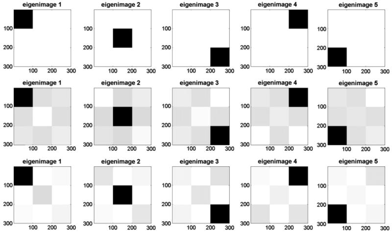
Grayscale images of the averages (top row), the 5th pointwise percentiles (middle row), and the 95th pointwise percentiles (bottom row) from the simulation study.

The total number of the normalized scores ξ_ik in this simulation study was 350,000 for each k. The left column of Fig. 3 shows the distribution of the true (generated) scores at the top and the distribution of the corresponding estimated scores at the bottom. We see that the EBLUPs recover the form of the underlying distributions. The accuracy of EBLUPs can be seen in the right column of Fig. 3 which shows the distribution of the differences between true and estimated scores. The top graph displays the boxplots of the differences. The bottom one shows the medians, 0.5%, 5%, 90% and 99.5% quantiles of the distribution of the difference. One very noticeable pattern here is the scores corresponding to the eigenimages with lower variances have larger spread due to a reduced signal to noise ratio. Results show that the EBLUPs estimate true scores very well.

Fig. 3.

Left panel shows the distribution of the true scores (top) and the estimated scores (bottom). Right panel shows the boxplots of the difference (ξ_ik−ξ̂_ik).Boxplots are given at the top. The bottom picture shows the medians (black marker), 5% and 95% quantiles (blue markers), and 0.5% and 99.5% quantiles (red markers). (For interpretation of the references to color in this figure legend, the reader is referred to the web version of this article.)

Fig. 4 shows the boxplots of the estimated eigenvalues. We display the centered and standardized eigenvalues, (σ̂_k−σ_k) / σ_k. The results indicate that eigenvalues are estimated with essentially no bias.

Fig. 4.

Boxplots of normalized estimated eigenvalues, (σ̂_k−σ_k)/σ_k. The zero is shown by the solid black line.

Application to RAVENS images

In this section we apply our method to the RAVENS images described in Motivating data section. The RAVENS images are 256 × 256 × 198 dimensional for 352 subjects, each with two visits roughly five years apart. We analyze visit 1 and visit 2 separately. In addition, to identify the principal directions of the longitudinal change we consider a difference between images taken at visit 1 and visit 2. Although the data contains both white and gray matter as well as CSF, for illustration, the analysis is restricted only to the processed gray matter data. A small technical concern was of a few artifactual negative values in the data from the preprocessing. These voxels were removed from the analysis. After processing, the intersection of non-background voxels across images was collected. Such an intersection greatly reduced the dimension of the data matrix from ten billion numbers to two billion numbers divided as three million relevant voxels per subject per visit with seven hundred and four subject-visits.

Following Motivating data section all calculations were performed in such a way that only one of the manageable submatrices X̃^m needs to be stored in memory at any given moment. The data matrix, of size 704 by 3 million, was divided into 100 submatrices of size 704 by 30 thousand (ten million numbers each). Note that on lower-resource computers the only change would be to reduce the size of submatrices. All calculations repeated for each of the three data sets were performed in Matlab 2010a and took around 15 min for each set on a PC with a quad core i7-2.67 Ghz processor and 6 Gb of RAM memory.

In the analysis, we first estimated the mean by the empirical voxel-specific arithmetic average. The visit specific mean images are uniform over the template and simply convey the message that localized changes in morphometry within subgroups get averaged over. The same is true for the mean of the longitudinal differences. In our eigenimage analysis we de-mean the data by subtracting out these vectors and work with de-meaned matrix X̃.

Fig. 5 shows the proportions of morphometric variation explained by the first thirty eigenimages for visit 1, visit 2, and the longitudinal difference. Cumulatively, the first thirty eigenimages explain 46.6%, 45.7%, and 52.5% of variation in data for visit 1, visit 2, and the longitudinal difference, respectively. The way eigenvalues decay on the most right graph of Fig. 5 is a clear indication that the longitudinal changes can be accurately described by the first thirty principal components explaining more than half of the longitudinal variation. Although the number of principal components, N, is usually chosen to explain enough variation (Di et al., 2008), our primary interest is the first few which identify the regions of brain exhibiting the most morphometric variation. The pattern of the percentage decrease on all three graphs of Fig. 5 flattens out after approximately the first ten principal components. Therefore, we concentrate our analysis on the first ten principal components.

Fig. 5.

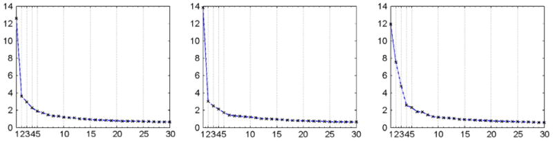
Proportions of morphometric variation explained by the first thirty eigenimages (from left to right: visit 1, visit 2, and the longitudinal difference).

Table 5 provides the cumulative percentages of variability explained by the first ten eigenimages. For visit 1 (top row) and visit 2 (middle row), they explain roughly the same amount of observed variation, 30%. For the longitudinal difference (bottom row), they explain 36.5% of the observed variability.

Table 5.

Labeled regions of the brain template. Abbreviations: PLICICPL = posterior limb of internal capsule including cerebral peduncle left, PLICICPR = posterior limb of internal capsule including cerebral peduncle right.

1	Medial front-orbital gyrus right
2	Middle frontal gyrus right
3	Lateral ventricle left
4	Insula right
5	Precentral gyrus right
6	Lateral front-orbital gyrus right
7	Cingulate region right
8	Lateral ventricle right
9	Medial frontal gyrus left
10	Superior frontal gyrus right
11	Globus pallidus right
12	Globus pallidus left
14	Putamen left
15	Inferior frontal gyrus left
16	Putamen right
17	Frontal lobe WM right
19	Angular gyrus right
23	Subthalamic nucleus right
25	Nucleus accumbens right
26	Uncus right
27	Cingulate region left
29	Fornix left
30	Frontal lobe WM left
32	Precuneus right
33	Subthalamic nucleus left
34	PLICICPL
35	PLICICPR
36	Hippocampal formation right
37	Inferior occipital gyrus left
38	Superior occipital gyrus right
39	Caudate nucleus left
41	Supramarginal gyrus left
43	Anterior limb of internal capsule left
45	Occipital lobe WM right
50	Middle frontal gyrus left
52	Superior parietal lobule left
53	Caudate nucleus right
54	Cuneus left
56	Precuneus left
57	Parietal lobe WM left
59	Temporal lobe WM right
60	Supramarginal gyrus right
61	Superior temporal gyrus left
62	Uncus left
63	Middle occipital gyrus right
64	Middle temporal gyrus left
69	Lingual gyrus left
70	Superior frontal gyrus left
72	Nucleus accumbens left
73	Occipital lobe WM left
74	Postcentral gyrus left
75	Inferior frontal gyrus right
80	Precentral gyrus left
83	Temporal lobe WM left
85	Medial front-orbital gyrus left
86	Perirhinal cortex right
88	Superior parietal lobule right
90	Lateral front-orbital gyrus left
92	Perirhinal cortex left
94	Inferior temporal gyrus left
95	Temporal pole left
96	Entorhinal cortex left
97	Inferior occipital gyrus right
98	Superior occipital gyrus left
99	Lateral occipitotemporal gyrus right
100	Entorhinal cortex right
101	Hippocampal formation left
102	Thalamus left
105	Parietal lobe WM right
108	Insula left
110	Postcentral gyrus right
112	Lingual gyrus right
114	Medial frontal gyrus right
118	Amygdala left
119	Medial occipitotemporal gyrus left
128	Anterior limb of internal capsule right
130	Middle temporal gyrus right
132	Occipital pole right
133	Corpus callosum
139	Amygdala right
140	Inferior temporal gyrus right
145	Superior temporal gyrus right
154	Middle occipital gyrus left
159	Angular gyrus left
165	Medial occipitotemporal gyrus right
175	Cuneus right
196	Lateral occipitotemporal gyrus left
203	Thalamus right
243	Background
251	Occipital pole left
254	Fornix right
255	Subarachnoid cerebro-spinal fluid

Top panel of Fig. 6 provides the estimated actual eigenvalues for the eigenimages. Notice, however, that we are more interested in the relative size of the eigenvalues representing quantitative measure of variability of the related eigenscores. Bottom panel of Fig. 6 plots the distributions of the eigenscores corresponding to the first ten eigenimages. In Single level FPCA section we showed that the estimates of the normalized eigenscores are given by the right singular vectors of matrix X̃. Therefore, the estimates of unnormalized eigenscores can be obtained once we multiply them by the square root of the corresponding eigenvalues provided in the top panel of Fig. 6. The estimated eigenscores serve as (signed) quantifiers relating eigenimages to subjects and their RAVENS maps.

Fig. 6.

Normalized distributions of the eigenscores corresponding to the first ten eigenimages (from left to right: visit 1, visit 2, and the longitudinal difference).

As we can see, the distribution of eigenscores in visit 1 and visit 2 are close to each other. Comparisons of the principal scores versus age are shown in Fig. 7. The results show how the major directions of volumetric variation are associated with cross-sectional baseline, age adjusted for height. The scores for the first component, being related to total gray matter volume simply display the well known decrease in overall volume with age. The final row displays that, adjusting for height, brain aging is progressive, with greater total volume declines with age. The other plots display non-significant relationship after having accounted for baseline height. Thus principal directions of gray matter volumetric variation appear unrelated to age and aging. The EBLUPs of the scores allow to perform more rigorous hypothesis testing of a specific scientific conjecture using relevant covariates.

Fig. 7.

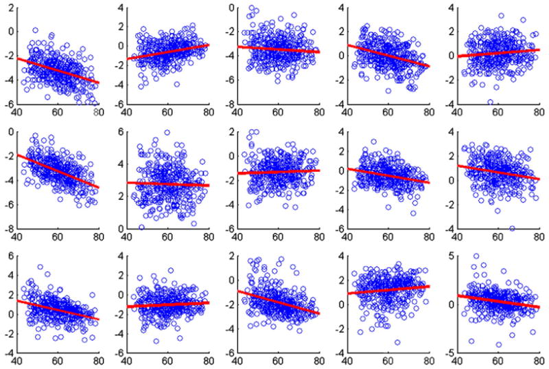
Plots of normalized eigenscores corresponding to the first 5 principal components against the age of the subjects adjusted for height. First row (visit 1), second row (visit 2), and third row (longitudinal difference). Red lines show fitted least squares lines adjusted for height. (For interpretation of the references to color in this figure legend, the reader is referred to the web version of this article.)

We now discuss overlap of the eigenimages with anatomical regions. Due to space limitations we discuss and depict only the first three eigenimages. We consider two independent separations of eigenimages. The first one quantifies the amount of variation of parcellated regions in template space. The kth eigenimage explains ${\sigma }_k={\sigma }_k{\varphi }_k^{\prime }{\varphi }_k$ amount of variation. Recall, each coordinate of ϕ_k corresponds to a voxel in template space. Therefore, if the template is parcellated into R regions, then we can calculate the proportion of the variance explained by this particular region within eigenimage ϕ_k–on a scale from 0 to 1. Formally, all unfolded voxels {1,…,p} of template space can be regrouped as a union of R nonoverlapping subsets of voxels {Reg₁,…,Reg_R}, where Reg_r consists of all region r voxels. Then eigenimage ϕ_k(v) can be represented as ${\varphi }_k(v)={\sum }_{r=1}^{R}I\{v\in {\mathit{\text{Reg}}}_r\}{\varphi }_k(v)$, where indicator I{v ε Reg_r} equals 1 if voxel v belongs to region r and equals 0 otherwise. Therefore, the variance explained by the kth eigenimage can be further decomposed as ${\sigma }_k={\sigma }_k{\mathit{\sum }}_{r=1}^R{W}_{\mathrm{kr}}$, where non-negative weights $W_{\mathrm{kr}}={\mathit{\sum }}_{v\in {\mathit{\text{Reg}}}_r}{\varphi }_k^2(v)$. Weights W_kr sum over the R regions to one and represent the proportions of variance σ_k explained by the regions. The second separation of eigenimages takes into account the sign of voxel values. Each eigenimage ϕ_k(v) can be split into two parts as ${\varphi }_k(v)={\varphi }_k^{\mathit{\text{pos}}}(v)+{\varphi }_k^{\mathit{\text{neg}}}(v)$, where ${\varphi }_k^{\mathit{\text{pos}}}(v)={\varphi }_k(v)I\{{\varphi }_k(v)\ge 0\}$ is the positive loading and ${\varphi }_k^{\mathit{\text{neg}}}(v)={\varphi }_k(v)I\{{\varphi }_k(v)<0\}$ is the negative loading. Note that because of sign invariance of SVD, the separation between positive and negative loadings is comparable only within an eigenimage. Subject i is loaded on the kth eigenimage through score ξ_ik. Therefore, subject i total loading can be split into the positive and negative parts as ${\mathrm{\xi }}_{\mathit{\text{ik}}}{\varphi }_k(v)={\mathrm{\xi }}_{\mathit{\text{ik}}}{\varphi }_k^{\mathit{\text{pos}}}(v)+{\mathrm{\xi }}_{\mathit{\text{ik}}}{\varphi }_k^{\mathit{\text{neg}}}(v)$. In other words, for principal score ξ_ik negative and positive voxel values correspond to the opposite directions (loadings) of variation. In our study, the template has been divided into R = 91 regions displayed in Table 5. However, the approach is general and applicable to any parcellation. In Table 2 we provide the variance explained by the labeled regions of the template for Visit 1. The twenty five regions with the highest loadings for each of the first three eigenimages are provided. Tables 1, 2, and 5 give now a way to determine a (signed) quantitative contribution of each particular region. For instance, the right middle temporal gyrus (130) explains 4.5% of the variance within eigenimage 1, which in turn explains 12.58% of the total variation. Hence, the right middle temporal gyrus explains 4.5% 12.58%= 0.57% of the total variation and has a mostly positive loading within eigenimage 1. Similarly, Tables 3 and 4 provide the regional quantifications of explained variation for Visit 2 and the longitudinal difference, respectively.

Table 2.

Visit 1: Proportion of the variance explained by the regions of the template (see Table 5 for the template parcellation). The twenty five regions with the highest loadings are provided. Third column quantifies the positive loading (blue), and fourth column quantifies the negative loading (red).

Eigenimage 1				Eigenimage 2				Eigenimage 3
Label	Variance explained	Positive loading	Negative loading	Label	Variance explained	Positive loading	Negative loading	Label	Variance explained	Positive loading	Negative loading
255	0.0508	0.0508	0.0000	27	0.0222	0.0222	0.0000	255	0.0719	0.0540	0.0179
130	0.0450	0.0450	0.0000	30	0.0179	0.0170	0.0009	83	0.0295	0.0009	0.0287
17	0.0410	0.0410	0.0000	255	0.0175	0.0124	0.0051	165	0.0285	0.0240	0.0045
30	0.0399	0.0399	0.0000	17	0.0143	0.0134	0.0008	64	0.0275	0.0011	0.0265
59	0.0381	0.0380	0.0001	7	0.0129	0.0129	0.0000	102	0.0255	0.0255	0.0000
145	0.0331	0.0331	0.0000	83	0.0124	0.0114	0.0010	95	0.0254	0.0000	0.0254
83	0.0298	0.0297	0.0000	59	0.0097	0.0085	0.0012	203	0.0235	0.0235	0.0000
61	0.0287	0.0287	0.0000	203	0.0073	0.0041	0.0032	30	0.0212	0.0180	0.0032
64	0.0268	0.0268	0.0000	6	0.0072	0.0072	0.0000	99	0.0202	0.0026	0.0177
27	0.0237	0.0237	0.0000	196	0.0066	0.0022	0.0044	108	0.0200	0.0199	0.0001
99	0.0221	0.0221	0.0000	105	0.0059	0.0055	0.0004	17	0.0185	0.0160	0.0025
2	0.0205	0.0205	0.0000	102	0.0059	0.0004	0.0054	94	0.0181	0.0025	0.0156
7	0.0201	0.0201	0.0000	3	0.0058	0.0058	0.0000	92	0.0176	0.0000	0.0176
75	0.0197	0.0197	0.0000	57	0.0057	0.0052	0.0005	21	0.0176	0.0000	0.0176
196	0.0187	0.0187	0.0000	90	0.0052	0.0052	0.0000	119	0.0172	0.0106	0.0066
119	0.0166	0.0166	0.0000	64	0.0051	0.0049	0.0001	196	0.0169	0.0071	0.0097
15	0.0158	0.0158	0.0000	119	0.0050	0.0017	0.0033	4	0.0158	0.0157	0.0001
105	0.0155	0.0154	0.0001	8	0.0050	0.0050	0.0000	59	0.0157	0.0048	0.0109
57	0.0150	0.0150	0.0000	75	0.0049	0.0047	0.0002	61	0.0118	0.0016	0.0101
165	0.0148	0.0148	0.0000	133	0.0047	0.0046	0.0001	88	0.0114	0.0103	0.0012
50	0.0147	0.0147	0.0000	61	0.0045	0.0031	0.0015	75	0.0114	0.0113	0.0001
4	0.0146	0.0146	0.0000	52	0.0045	0.0042	0.0003	114	0.0111	0.0107	0.0004
5	0.0144	0.0144	0.0000	99	0.0039	0.0025	0.0015	5	0.0108	0.0104	0.0004
108	0.0141	0.0141	0.0000	20	0.0039	0.0000	0.0039	145	0.0105	0.0100	0.0005
74	0.0116	0.0116	0.0000	32	0.0036	0.0036	0.0000	9	0.0100	0.0096	0.0004

Table 1.

Cumulative percentage of variation explained by first ten eigenimages for RAVENS data (visit 1 (top row), visit 2 (middle row), and the longitudinal difference (bottom row)).

Visit 1
Component	1	2	3	4	5	6	7	8	9	10
Cum % var	12.58	16.20	19.15	21.42	23.31	25.00	26.47	27.81	29.11	30.29
Visit 2
Component	1	2	3	4	5	6	7	8	9	10
Cum % var	13.81	16.82	19.30	21.43	23.15	24.57	25.92	27.22	28.48	29.68
Longitudinal difference
Component	1	2	3	4	5	6	7	8	9	10
Cum % var	11.91	19.44	24.21	26.80	29.09	30.91	32.70	34.16	35.42	36.60

Table 3.

Visit 2: Proportion of the variance explained by the regions of the template (see Table 5 for the template parcellation). The twenty five regions with the highest loadings are provided. Third column quantifies the positive loading (blue), and fourth column quantifies the negative loading (red).

Eigenimage 1				Eigenimage 2				Eigenimage 3
Label	Variance explained	Positive loading	Negative loading	Label	Variance explained	Positive loading	Negative loading	Label	Variance explained	Positive loading	Negative loading
255	0.0542	0.0542	0.0000	255	0.0425	0.0120	0.0306	255	0.0612	0.0500	0.0113
30	0.0438	0.0437	0.0001	99	0.0274	0.0258	0.0016	30	0.0342	0.0132	0.0211
17	0.0420	0.0419	0.0001	30	0.0165	0.0004	0.0161	17	0.0251	0.0061	0.0190
130	0.0390	0.0390	0.0000	165	0.0165	0.0066	0.0099	27	0.0222	0.0006	0.0215
59	0.0338	0.0336	0.0002	196	0.0153	0.0120	0.0033	83	0.0220	0.0015	0.0205
145	0.0307	0.0307	0.0000	17	0.0144	0.0005	0.0139	88	0.0218	0.0174	0.0043
61	0.0288	0.0288	0.0000	108	0.0137	0.0000	0.0137	105	0.0206	0.0059	0.0147
83	0.0275	0.0273	0.0002	119	0.0136	0.0107	0.0030	108	0.0189	0.0141	0.0047
64	0.0268	0.0268	0.0000	4	0.0129	0.0000	0.0129	64	0.0182	0.0005	0.0177
27	0.0214	0.0214	0.0000	203	0.0123	0.0000	0.0123	7	0.0178	0.0002	0.0176
2	0.0207	0.0207	0.0000	102	0.0115	0.0000	0.0115	61	0.0156	0.0061	0.0095
75	0.0187	0.0187	0.0000	15	0.0107	0.0000	0.0107	59	0.0141	0.0018	0.0123
7	0.0180	0.0180	0.0000	83	0.0099	0.0088	0.0011	165	0.0137	0.0126	0.0011
99	0.0174	0.0174	0.0000	75	0.0098	0.0000	0.0098	52	0.0125	0.0095	0.0030
50	0.0173	0.0173	0.0000	114	0.0084	0.0000	0.0084	57	0.0125	0.0025	0.0099
15	0.0170	0.0170	0.0000	59	0.0083	0.0049	0.0035	203	0.0119	0.0119	0.0000
105	0.0167	0.0165	0.0002	64	0.0082	0.0053	0.0029	102	0.0111	0.0111	0.0000
196	0.0166	0.0166	0.0000	95	0.0078	0.0078	0.0000	19	0.0110	0.0059	0.0050
57	0.0166	0.0165	0.0001	145	0.0076	0.0003	0.0073	130	0.0105	0.0023	0.0082
5	0.0148	0.0148	0.0000	9	0.0066	0.0000	0.0065	196	0.0091	0.0060	0.0031
165	0.0143	0.0143	0.0000	88	0.0065	0.0002	0.0063	4	0.0090	0.0051	0.0039
119	0.0133	0.0133	0.0000	94	0.0064	0.0050	0.0014	14	0.0089	0.0089	0.0000
74	0.0132	0.0132	0.0000	92	0.0062	0.0062	0.0000	9	0.0085	0.0067	0.0019
4	0.0130	0.0130	0.0000	130	0.0057	0.0020	0.0037	95	0.0082	0.0000	0.0082
108	0.0128	0.0128	0.0000	5	0.0054	0.0002	0.0052	92	0.0082	0.0000	0.0082

Table 4.

Longitudinal difference: Proportion of the variance explained by the regions of the template (see Table 5 for the template parcellation). The twenty five regions with the highest loadings are provided. Third column quantifies the positive loading (blue), and fourth column quantifies the negative loading (red).

Eigenimage 1				Eigenimage 2				Eigenimage 3
Label	Variance explained	Positive loading	Negative loading	Label	Variance explained	Positive loading	Negative loading	Label	Variance explained	Positive loading	Negative loading
255	0.0620	0.0029	0.0591	64	0.0188	0.0000	0.0188	255	0.0687	0.0087	0.0599
30	0.0439	0.0003	0.0436	255	0.0179	0.0014	0.0165	64	0.0636	0.0000	0.0636
17	0.0419	0.0003	0.0416	130	0.0142	0.0000	0.0142	94	0.0344	0.0000	0.0344
27	0.0341	0.0000	0.0341	94	0.0133	0.0000	0.0133	83	0.0288	0.0023	0.0265
59	0.0320	0.0000	0.0320	83	0.0077	0.0008	0.0069	17	0.0259	0.0192	0.0067
145	0.0291	0.0000	0.0291	196	0.0070	0.0000	0.0070	30	0.0239	0.0058	0.0180
61	0.0283	0.0000	0.0283	102	0.0066	0.0066	0.0000	21	0.0227	0.0000	0.0227
83	0.0257	0.0000	0.0257	21	0.0060	0.0000	0.0060	130	0.0218	0.0021	0.0196
130	0.0235	0.0000	0.0235	30	0.0048	0.0008	0.0040	90	0.0190	0.0002	0.0189
7	0.0231	0.0000	0.0231	140	0.0047	0.0000	0.0047	95	0.0178	0.0000	0.0178
75	0.0211	0.0000	0.0211	59	0.0046	0.0011	0.0035	61	0.0171	0.0002	0.0169
4	0.0196	0.0000	0.0196	61	0.0044	0.0001	0.0043	140	0.0151	0.0004	0.0148
108	0.0179	0.0000	0.0179	50	0.0040	0.0000	0.0040	59	0.0145	0.0083	0.0062
64	0.0174	0.0000	0.0174	37	0.0040	0.0000	0.0040	4	0.0144	0.0144	0.0000
6	0.0169	0.0000	0.0169	17	0.0035	0.0012	0.0023	5	0.0118	0.0066	0.0052
99	0.0167	0.0000	0.0167	95	0.0031	0.0000	0.0031	6	0.0115	0.0004	0.0111
105	0.0160	0.0001	0.0159	52	0.0027	0.0002	0.0025	16	0.0098	0.0098	0.0000
57	0.0153	0.0001	0.0152	251	0.0025	0.0000	0.0025	15	0.0097	0.0009	0.0088
88	0.0149	0.0001	0.0148	145	0.0023	0.0003	0.0020	102	0.0097	0.0097	0.0000
90	0.0149	0.0000	0.0149	203	0.0023	0.0023	0.0000	75	0.0090	0.0076	0.0014
2	0.0145	0.0000	0.0145	90	0.0022	0.0003	0.0019	50	0.0088	0.0001	0.0088
52	0.0143	0.0000	0.0143	99	0.0021	0.0000	0.0021	154	0.0083	0.0000	0.0083
114	0.0141	0.0004	0.0137	15	0.0020	0.0000	0.0019	99	0.0080	0.0053	0.0027
196	0.0141	0.0001	0.0139	70	0.0019	0.0000	0.0019	145	0.0080	0.0073	0.0006
15	0.0137	0.0000	0.0137	6	0.0019	0.0005	0.0013	196	0.0079	0.0011	0.0069

As we showed in the Introduction section the estimated principal components (eigenimages) are left singular vectors of matrix X̃. Each left singular vector is of size p≈3·10⁶ unfolded voxels. Therefore, each voxel is represented by a small value between negative and positive one and squares of the voxel values are summed to one. The distribution of the negative and positive voxel loadings are presented in Fig. 8 in red and blue, respectively. The voxel values of the estimated eigenimage ϕ̂ = (ϕ̂₁,…,ϕ̂_p) were transformed as ϕ̂→256·(ϕ̂−min_sϕ̂_s)/(max_sϕ̂_s−min_sϕ̂_s) separately for voxels with positive and negative loadings. The transformed negative and positive loadings overlaid with the template are presented in Figs. 9, 10, and 11. Note that our approach does not incorporate spatial structure or smoothness. In part, this has been taken into account at the preprocessing step when a 3D Gaussian kernel had been used to smooth original brain images. However, the found eigenimages obey some regional boundaries despite the above-mentioned ignorance of spatial relationships. We believe that it highlights considerable potential of the methods within these settings.

Fig. 8.

Distributions of the intensities of the first three eigenimages (visit 1 (top row), visit 2 (middle row), and the longitudinal difference (bottom row)). (For interpretation of the references to color in this figure legend, the reader is referred to the web version of this article.)

Fig. 9.

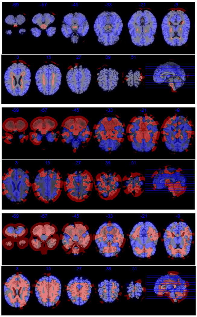
The first three estimated eigenimages for visit 1. Each eigenimage is represented by eleven equidistant axial slices. Negative loadings are depicted in red, and positive ones are in blue. (For interpretation of the references to color in this figure legend, the reader is referred to the web version of this article.)

Fig. 10.

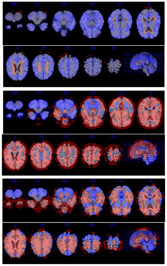
The first three estimated eigenimages for visit 2. Each eigenimage is represented by eleven equidistant axial slices. Negative loadings are depicted in red, and positive ones are in blue. (For interpretation of the references to color in this figure legend, the reader is referred to the web version of this article.)

Fig. 11.

The first three estimated eigenimages for the longitudinal difference. Each eigenimage is represented by eleven equidistant axial slices. Negative loadings are depicted in red, and positive ones are in blue. (For interpretation of the references to color in this figure legend, the reader is referred to the web version of this article.)

Discussion

In this paper we proved a connection between SVD and FPCA models. This coupling allowed us to develop efficient model-based computing techniques. The developed approach was applied to a novel morphometric data set with 704 RAVENS images. Principal components of morphometric variation were identified and studied. An alternative to our analysis would be a more formal separation of cross-sectional and longitudinal morphometric variation within multilevel functional principal component analysis framework suggested in Di et al. (2008).

There are a few important limitations in the presented methodology. First, we have not assumed noise in the model. RAVENS data represent preprocessed and smoothed images. However, there are a considerable number of studies collecting functional observations measured with non-ignorable noise. The ideas proposed in Huang et al. (2008) and Eilers et al. (2006) can be explored to develop a feasible smoothing procedure for spatial principal components. Another related development could be a rigorous incorporation of 3D spatial structure.

Our model assumes that the functional data are densely, rather than sparsely, observed. The issue of sparsity was addressed in Di et al. (2008) and Di and Crainiceanu (2010) for multilevel models. The proposed efficient solutions were based on smoothing of the covariance operator which is infeasible for high-dimensional data. Therefore, there is a great demand in computationally efficient procedures of covariance smoothing in the high dimensional context.

References

- Ashburner J, Friston K. Voxel-based morphometry–the methods. Neuroimage. 2000;11:805–821. doi: 10.1006/nimg.2000.0582. [DOI] [PubMed] [Google Scholar]
- Beckmann C, Smith S. Tensorial extensions of independent component analysis for multisubject fMRI analysis. Neuroimage. 2005;25:294–311. doi: 10.1016/j.neuroimage.2004.10.043. [DOI] [PubMed] [Google Scholar]
- Caffo B, Crainiceanu C, Verduzco G, Joel S, Mostofsky SH, Bassett SS, Pekar JJ. Two-stage decompositions for the analysis of functional connectivity for fMRI with application to Alzheimer's disease risk. Neuroimage. 2010;51:1140–1149. doi: 10.1016/j.neuroimage.2010.02.081. [DOI] [PMC free article] [PubMed] [Google Scholar]
- Crainiceanu CM, Caffo BS, Luo S, Zipunnikov VV, Punjabi NM. Population Value Decomposition, a framework for the analysis of image populations. Johns Hopkins University, Dept of Biostatistics Working Paper 220. 2010 doi: 10.1198/jasa.2011.ap10089. [DOI] [PMC free article] [PubMed] [Google Scholar]
- Crainiceanu CM, Staicu AM, Di CZ. Generalized multilevel functional regression. J Am Stat Assoc. 2009;104(488):1550–1561. doi: 10.1198/jasa.2009.tm08564. [DOI] [PMC free article] [PubMed] [Google Scholar]
- Davatzikos C, Fan Y, Wu X, Shen D, Resnick SM. Detection of prodromal Alzheimer's disease via pattern classification of magnetic resonance imaging. Neurobiol Aging. 2008;29:514–523. doi: 10.1016/j.neurobiolaging.2006.11.010. [DOI] [PMC free article] [PubMed] [Google Scholar]
- Demidenko . Mixed Models: Theory and Applications. John Wiley and Sons; 2004. [Google Scholar]
- Di CZ, Crainiceanu CM. Multilevel sparse functional principal component analysis. Technical Report. 2010 doi: 10.1002/sta4.50. [DOI] [PMC free article] [PubMed] [Google Scholar]
- Di CZ, Crainiceanu CM, Caffo BS, Punjabi NM. Multilevel functional principal component analysis. Ann Appl Stat. 2008;3(1):458–488. doi: 10.1214/08-AOAS206SUPP. [DOI] [PMC free article] [PubMed] [Google Scholar]
- Eilers PH, Currie ID, Durban M. Fast and compact smoothing on large multidimensional grids. Comput Stat Data Anal. 2006;50:61–76. [Google Scholar]
- Goldszal A, Davatzikos C, Pham D, Yan M, Bryan R, Resnick SM. An image processing protocol for the analysis of MR images from an elderly population. J Comput Assist Tomogr. 1998;22:827–837. doi: 10.1097/00004728-199809000-00030. [DOI] [PubMed] [Google Scholar]
- Golub GH, Loan CV. Matrix Computations. The Johns Hopkins University Press; 1996. [Google Scholar]
- Greven S, Crainiceanu CM, Caffo BS, Reich D. Longitudinal functional principal component analysis. Electron J Stat. 2010;4:1022–1054. doi: 10.1214/10-EJS575. [DOI] [PMC free article] [PubMed] [Google Scholar]
- Guo W. Functional mixed effects models. Biometrics. 2002;58:121–128. doi: 10.1111/j.0006-341x.2002.00121.x. [DOI] [PubMed] [Google Scholar]
- Harville D. Extension of the Gauss–Markov theorem to include the estimation of random effects. Ann Stat. 1976;4(2):384–395. [Google Scholar]
- Huang JZ, Shen H, Buja A. Functional principal components analysis via penalized rank one approximation. Electron J Stat. 2008;2:678–695. [Google Scholar]
- Joliffe I. Principal Component Analysis. 2nd. Springer-Verlag; New-York: 2002. [Google Scholar]
- Karhunen K. Uber Lineare Methoden in der Wahrscheinlichkeitsrechnung. Ann Acad Sci Fenn. 1947;37:1–79. [Google Scholar]
- McCulloch C, Searle S. Generalized, Linear, and Mixed Models. Wiley Interscience; 2001. [Google Scholar]
- Mohamed A, Davatzikos C. Shape representation via best orthogonal basis selection. Med Image Comput Comput Assist Interv. 2004;3216:225–233. [Google Scholar]
- Morris JS, Carroll RJ. Wavelet-based functional mixed models. J R Stat Soc B. 2006;68:179–199. doi: 10.1111/j.1467-9868.2006.00539.x. [DOI] [PMC free article] [PubMed] [Google Scholar]
- Ramsay J, Silverman B. Functional Data Analysis. 2nd. Springer; 2005. [Google Scholar]
- Reiss P, Ogden RT. Functional generalized linear models with applications to neuroimaging. Poster Presentation Workshop on Contemporary Frontiers in High-Dimensional Statistical Data Analysis 2008 [Google Scholar]
- Reiss P, Ogden RT. Functional generalized linear models with images as predictors. Biometrics. 2010;1:61–69. doi: 10.1111/j.1541-0420.2009.01233.x. [DOI] [PubMed] [Google Scholar]
- Reiss PT, Ogden RT, Mann J, Parsey RV. Functional logistic regression with PET imaging data: a voxel-level clinical diagnostic tool. J Cereb Blood Flow Metab. 2005;25:s635. [Google Scholar]
- Resnick S, Espeland MA, Jaramillo SA, Hirsch C, Stefanick ML, Murray AM, Ockene J, Davatzikos C. Postmenopausal hormone therapy and regional brain volumes: the WHIMS-MRI Study. Neurology. 2009;72:135–142. doi: 10.1212/01.wnl.0000339037.76336.cf. [DOI] [PMC free article] [PubMed] [Google Scholar]
- Schwartz B, Stewart W, Bolla K, Simon D, Bandeen-Roche K, Gordon B, Links J, Todd A. Past adult lead exposure is associated with longitudinal decline in cognitive function. Neurology. 2000a;55:1144. doi: 10.1212/wnl.55.8.1144. [DOI] [PubMed] [Google Scholar]
- Schwartz B, Stewart W, Kelsey K, Simon D, Park S, Links J, Todd A. Associations of tibial lead levels with BsmI polymorphisms in the vitamin D receptor in former organolead manufacturing workers. Environ Health Perspect. 2000b;108:199. doi: 10.1289/ehp.00108199. [DOI] [PMC free article] [PubMed] [Google Scholar]
- Shen DG, Davatzikos C. Very high resolution morphometry using mass-preserving deformations and HAMMER elastic registration. Neuroimage. 2003;18:28–41. doi: 10.1006/nimg.2002.1301. [DOI] [PubMed] [Google Scholar]
- Staicu AM, Crainiceanu CM, Carroll RJ. Fast analysis of spatially correlated multilevel functional data. Biostatistics. 2010;11(2):177–194. doi: 10.1093/biostatistics/kxp058. [DOI] [PMC free article] [PubMed] [Google Scholar]
- Stewart W, Schwartz B, Simon D, Bolla K, Todd A, Links J. Neurobehavioral function and tibial and chelatable lead levels in 543 former organolead workers. Neurology. 1999;52:1610. doi: 10.1212/wnl.52.8.1610. [DOI] [PubMed] [Google Scholar]
- Xue Z, Shen D, Davatzikos C. CLASSIC: consistent longitudinal alignment and segmentation for serial image computing. Neuroimage. 2006;30:388–399. doi: 10.1016/j.neuroimage.2005.09.054. [DOI] [PubMed] [Google Scholar]
- Yao F, Muller HG, Wang JL. Functional data analysis for sparse longitudinal data. J Am Stat Assoc. 2005;100:577–590. [Google Scholar]
- Zhang L, Marron J, Shen H, Zhu Z. Singular value decomposition and its visualization. J Comput Graphical Stat. 2007;16:833–854. [Google Scholar]