

Abstract
Atherosclerosis is a complex disease whose spatial distribution is hypothesized to be influenced by the local hemodynamic environment. The use of transgenic mice provides a mechanism to study the relationship between hemodynamic forces, most notably wall shear stress (WSS), and the molecular factors that influence the disease process. Phase contrast MRI using rectilinear trajectories has been used to measure boundary conditions for use in computational fluid dynamic models. However, the unique flow environment of the mouse precludes use of standard imaging techniques in complex, curved flow regions such as the aortic arch. In this paper two-dimensional and three-dimensional spiral cine phase contrast sequences are presented that enable measurement of velocity profiles in curved regions of the mouse vasculature. WSS is calculated directly from the spatial velocity gradient, enabling WSS calculation with a minimal set of assumptions. In contrast to the outer radius of the aortic arch, the inner radius has a lower time-averaged longitudinal WSS (7.06±0.76 dyne/cm2 v. 18.86±1.27 dyne/cm2; p<0.01) and higher oscillatory shear index (0.14±0.01 v. 0.08±0.01; p<0.01). This finding is in agreement with humans, where WSS is lower and more oscillatory along the inner radius, an atheroprone region, than the outer radius, an atheroprotective region.
Keywords: spiral, phase contrast, mouse, wall shear stress, MRI
Atherosclerosis is an inflammatory disease of the wall of large arteries resulting in the development of lesions and the narrowing of blood vessels (1,2). The focal development of atherosclerosis correlates to the complex hemodynamic environment at branch points and regions of high curvature. Wall shear stress (WSS), the shear force experienced by the vessel wall due to blood flow within the lumen, is believed to be a primary factor in the development of atherosclerotic plaques. Atherosclerotic plaques predominantly occur in regions with low, oscillatory WSS (3,4).
Manipulation of the mouse genome has enabled the detailed investigation of the role of specific genes in complex disease processes. Transgenic mice, specifically apolipoprotein E knockout (ApoE−/−) mice, have proven invaluable in the study of atherosclerosis (5–9). Using transgenic mice and imaging, the potential exists for probing the relationship between WSS and the molecular factors involved in atherosclerosis in vivo.
Multiple imaging modalities have been proposed to measure WSS in small animals including ultrasound (10) and magnetic resonance imaging (MRI) (11,12). Flow measurements made with ultrasound and/or MRI can be used as boundary conditions for computational fluid dynamic (CFD) models of blood flow in the mouse vasculature. CFD approaches are advantageous due to their ability to estimate WSS at a high resolution with only a few measurements. However, the models are limited by their assumptions and their ability to model higher order effects such as vessel wall compliance. The use of direct calculation of WSS in regions of curved vasculature has been reported in humans (13); however it has yet to be reported in small animal studies.
In theory, phase contrast (PC) MRI can measure every vector component of velocity in any oblique spatial orientation and at any depth in the mouse, potentially making it an ideal method for measuring WSS. However, in practice, the specific flows encountered in the mouse create severe artifacts when traditional rectilinear trajectories are used. Blood velocities in the mouse aortic arch are comparable to blood velocities found in human aortic arch (~100 cm/sec), yet the anatomy is an order of magnitude smaller. These fast flows through small and complex anatomy result in displacement artifacts and signal loss comparable to stenotic jets in humans (14). Movement of blood between excitation and data acquisition causes displacement artifacts, and their severity is proportional to the echo time (TE) and the amount of in-plane motion. Signal loss is a result of phase dispersion across a voxel and its severity is proportional to the gradient moments, the velocity gradient, and pixel size.
Spiral k-space trajectories have desirable properties with respect to signal-to-noise ratio (SNR), efficiency, and flow properties (15,16). Since a readout prephaser is not needed, spiral trajectories have a short TE and therefore have reduced displacement artifacts. Spiral MRI has successfully been applied to humans (14,17,18); however special considerations are necessary when applying spiral trajectories at high field strength. Off-resonance effects increase with field strength and lead to increased blurring. Gradient fidelity errors, and therefore k-space trajectory errors, occur when fast slew rates (>500 mT/m/ms) are used and result in image artifacts. In this work, short duration spiral readouts along with k-space trajectory measurements will be investigated to overcome blurring and gradient fidelity errors, respectively.
A two-dimensional spiral cine PC sequence and a three-dimensional stack-of-spirals cine PC sequence are presented for measuring the hemodynamic environment of the mouse aorta. The dataset is then automatically segmented and WSS calculated via direct evaluation of the velocity gradient near the vessel wall. The methods are then used to measure and describe the hemodynamic environment in ApoE−/− mice.
Methods
Imaging was performed on a 7.0T MR system (Clinscan, Bruker Biospin, Ettlingen, Germany) using a 30 mm diameter cylindrical birdcage radiofrequency coil and an MR-compatible physiological monitoring and gating system for mice (SA Instruments, Inc., Stony Brook, NY). Maximum gradient strength of the system was 500 mT/m and the peak slew rate achievable was 6667 mT/m/ms. Mice were anesthetized using 1.25% isoflurane in oxygen and body temperature was maintained at 37° using thermostated circulating water. All animals were used in accordance with a protocol approved by the animal care and use committee at our institution.
Comparison of rectilinear and spiral trajectories for PC MRA of the mouse aorta
To investigate the effects of k-space trajectory on flow artifacts in the mouse aorta, a two-dimensional rectilinear and two-dimensional spiral trajectory were compared. Wild-type mice (C57BL6, Jackson Laboratory) were imaged at two locations within the mouse; in a straight region (thoracic aorta) and in a region with complex, curved flows (aortic root). The sequences were designed to minimize TE subject to imaging constraints and hardware limitations. The spiral sequence achieved a minimum TE of 0.86 ms. However, the need for a readout prephaser gradient in the rectilinear scan increased the TE to 3.49 ms.
Imaging constraints were chosen by empirical experimentation based on image quality, spatial resolution, temporal resolution, and total image acquisition time. Balanced velocity encodings with positive velocity encoding and negative velocity encoding in the through-plane direction were alternated between heart beats using a 120 cm/s velocity encoding (VENC). The VENC was chosen above the maximum expected velocity to avoid phase wrap. Images were acquired with 100 μm in-plane resolution to achieve sufficient resolution across the lumen of the aorta. Twelve cardiac phases were acquired with an 8 ms TR. Additional imaging parameters were a 25.6 × 25.6 mm2 FOV and 1 mm slice thickness.
Image blurring due to off-resonance effects increases linearly with field strength, so the use of spirals at 7T requires a combination of short readouts and deblurring techniques. Readouts were limited to 2 ms, requiring 100 imaging interleaves to Nyquist sample k-space. An additional 28 interleaves were used to acquire a low-resolution field map for use in linear field map off-resonance correction to further decrease blurring effects (19).
To keep the total scan time constant for the sequences, the spiral sequence used eight averages and the rectilinear sequence used four averages. The spiral sequence used more averages due to the increased scan efficiency of the spiral trajectories. To keep within duty cycle limits, data was collected on alternating heartbeats to allow for gradient cooling. Total scan time for both sequences was approximately 8 minutes, depending on heart rate.
3D Stack of Spirals Cine Phase Contrast
Two-dimensional acquisitions provide localized information regarding hemodynamic forces and flow rates. Multiple 2D acquisitions to cover a 3D volume would be time prohibitive. Additionally, the difficulty in localizing a slice perpendicular to the flow direction in curved vessels such as the aortic arch can lead to experimental error. In order to characterize the complete hemodynamic environment throughout the aortic arch a three-dimensional acquisition is needed.
A stack-of-spirals trajectory was used to acquire a three-dimensional volume in five 24-week old ApoE−/− mice (Jackson Laboratory). A schematic of the sequence is shown Figure 1. Velocity in the x, y, and z direction (vx, vy, and vz respectively) were measured with a VENC of 120 cm/s using balanced four-point encoding. The four encoding sets used were (−vx, −vy, −vz), (+vx,+vy, −vz), (+vx, −vy, +vz), and (−vx, +vy, +vz) where the sign indicates whether the positive or negative velocity encoding was performed (20). A single encoding set was acquired each heartbeat, thereby requiring four separate heartbeats to measure one set of velocity encodings for each spiral interleaf. Isotropic 170 μm resolution was achieved over a 32.64 × 32.64 × 5.44 mm3 FOV and 192 × 192 × 32 acquisition matrix. A slice oversampling of 25% was empirically found to prevent wrap around artifacts in the second phase-encoding direction. Fourteen frames were acquired across the cardiac cycle at a 6.5 ms TR and 850 μs TE. A 15° sinc excitation pulse was used to excite a volume superior to the left ventricle. The close proximity of the venous and arterial systems can result in poor vessel contrast and complicates the segmentation of the aortic arch. For this reason, a saturation band was placed above the excitation volume to saturate incoming venous blood from the superior vena cava.
Figure 1.

Timing diagram for the spiral 3D cine PC sequence. N images are acquired across the cardiac cycle (indicated by Phs. 1 to Phs. N in the diagram) following detection of the QRS complex in the EKG. Dotted lines indicate alternating velocity encodings and arrows are used to indicate partition-encoding and rewinding gradients. Gradients are not drawn to scale for ease of visualization. Spoiler gradients are played off-axis to the slab direction to minimize the gradient duty cycle.
Although spiral trajectories have many desirable flow properties, when velocities are sufficiently large and the total movement of a spin on the same axes as a spiral readout is on the order of a pixel size a misregistration of the spatial encoding frequencies can occur (21). This misregistration leads to an asymmetric point spread function that can create image artifacts. In a three-dimensional acquisition of the aortic arch, the primary flow direction is no longer necessarily orthogonal to the spiral readouts and this effect cannot be avoided. To reduce the misregistration artifact, ultra-short 900 μs readouts were used. This had the added benefit of eliminating the need for off-resonance correction but led to long scan times. To reduce scan time, variable density sampling (22) was used to reduce the number of necessary interleaves from 192 to 160 leading to a decrease in scan time of 20%. A linear reduction in k-space sampling with radial k-space distance was used to fully sample the center of k-space and undersample by 16% the edge of k-space. The total scan duration is dependent on HR and ranges from 42 minutes for a HR of 600 bpm to 53 minutes for a HR of 480 bpm.
Gradient duty cycle limitations placed constraints on the image orientation, partition encoding order, and gradient spoiling. A true axial imaging orientation was used to minimize the maximum gradients played on any axis. To limit time spent at the edges of k-space, where the gradient demands are greatest, partition encoding was acquired using a low duty cycle interleaved reordering. Finally, gradient spoilers were played on axes other than the partition axis where the majority of large gradient events occur.
Gridding during spiral image reconstruction requires accurate knowledge of the k-space trajectory. Errors in the true k-space trajectory versus the prescribed k-space trajectory can be caused by gradient hardware imperfections, eddy currents, and gradient discretization. k-space trajectory errors manifest themselves as signal inhomogeneities and streak artifacts in the reconstructed image and are exacerbated by the increased spiral gradient slew rates (>500 mT/m/ms) necessary for the three-dimensional sequence. To account for trajectory errors, every spiral interleaf for every velocity encoding was first measured in a phantom (23,24). The measured trajectories were then used in image reconstruction for all subsequent acquisitions. Since all acquisitions were performed in the axial direction, it was not necessary to measure different spatial orientations of the spiral trajectories.
If the blood velocity is greater than the VENC, phase wrap occurs in the measured phase images. In the presence of noise, phase wrap can additionally occur in regions where blood velocity is below but near the VENC. Therefore every PC dataset was phase unwrapped using a path-following technique (25) prior to analysis. Following phase unwrapping, eddy current correction was performed by subtracting a linear fit to the phase image at diastole (26).
Calculation of WSS
WSS was directly calculated from the spatial velocity gradients at the vessel wall. Let vl, vr, and vc be the local longitudinal, radial, and circumferential components of velocity relative to the vessel wall. If blood is assumed to be a Newtonian fluid with viscosity μ, then instantaneous longitudinal WSS, τl, and circumferential WSS, τc, can be calculated according to
| [1] |
and
| [2] |
respectively. Prior to calculation of WSS however, the vessel wall must be segmented and the unit vectors in radial, r̂, longitudinal, l̂, and circumferential, ĉ, direction at each surface point must be defined.
The vessel wall was automatically segmented at each cardiac phase using an automatic segmentation method that incorporated the velocity data into the segmentation problem (27). To limit calculation of WSS to the aortic arch, branches were removed using a generalized cylinder fit (28). The segmentation algorithm produced a triangular mesh with nodes defined in the physical (x, y, z) coordinate system.
The local radial, longitudinal and circumferential directions were then calculated for each surface patch defined by the triangular mesh. The radial direction was defined as the inward normal to the surface patch. To calculate the circumferential direction, the aortic surface was skeletonized to find the centerline of the vessel (29). The closest point on the centerline to the midpoint of the surface patch was found and the cross product between the centerline point’s tangential vector, t̂, with the radial unit normal provided the circumferential direction, ĉ = t̂ × r̂. This resulted in a circumferential unit vector pointing clockwise with respect to the primary direction of flow as defined by the centerline. Finally, the longitudinal direction was calculated according to l̂ = r̂ × ĉ. A schematic of the described unit vectors is shown in Figure 2.
Figure 2.
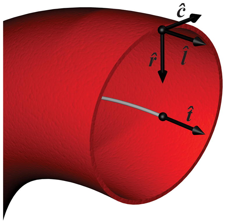
Schematic of the unit normal vectors in the radial, r̂, longitudinal, l̂, and circumferential, ĉ, direction at a representative surface point along with the tangential vector, t̂, at the vessel centerline. The blood vessel is shown in red and the vessel centerline by a grey line. The vessel is viewed looking upstream of the direction of blood flow.
Prior to calculation of the spatial velocity gradient, the velocity was zeroed outside the vessel lumen and spatially median filtered inside the lumen within a six-connectivity neighborhood. The spatial median filter acts to remove velocity outliers potentially created by segmentation errors, but leaves the data unchanged if it lies in a locally monotonic region. Similar to Stalder et al., PC data were fit with a cubic spline to allow direct evaluation of the spatial velocity gradients (30). However, instead of a separate Gaussian smoothing step, filtering was incorporated via a cubic smoothing spline. Using the cubic spline, Eqs. [1] and [2] were directly evaluated to compute both components of WSS for each surface point.
In addition to instantaneous WSS values, the time-averaged circumferential WSS, ; time-averaged longitudinal WSS; ; and time-averaged WSS magnitude, , were also calculated where T is the time period of one cardiac cycle.
The degree of variation in a WSS waveform is hypothesized to play a significant role in the spatial distribution of atherosclerotic plaques. The oscillatory shear index, OSI, was used to measure the degree of variability of the WSS waveform given in (31) as
| [3] |
where . A higher OSI corresponds to a more oscillatory flow.
The aorta was subdivided into twelve sectors for regional analysis. Each surface patch was defined according to longitudinal position (ascending aorta, top of the arch, descending aorta) and circumferential position (inner radius, anterior, posterior, and outer radius). WSS values and OSI values were averaged across each sector.
Statistical Analysis
Two-way ANOVA was used for determining statistical significance in instantaneous WSS values between different regions during the cardiac cycle. A paired t-test was used for comparison of time-averaged WSS values and the OSI. All values are reported as mean ± standard error.
Results
2D Spiral Cine PC
Figure 3 shows example magnitude and phase images for the rectilinear and spiral sequence in the thoracic aorta and aortic root. Both the rectilinear and spiral sequences succeed in measuring the velocity data in the thoracic aorta where velocities are slower and the vessel geometry is straight. However, at the aortic root, where velocities are higher and the vessel geometry is curved, the rectilinear sequence suffers from signal loss within the vessel lumen due to displacement artifacts and phase cancellation. In Figure 4 the measured flow rates are shown from a representative wild-type mouse at the aortic root and thoracic aorta measured with both pulse sequences. Similar flow waveforms are found using both techniques within the thoracic aorta. However, at the aortic root the rectilinear sequence fails to measure the flow during systole while the spiral sequence captures the entire waveform.
Figure 3.
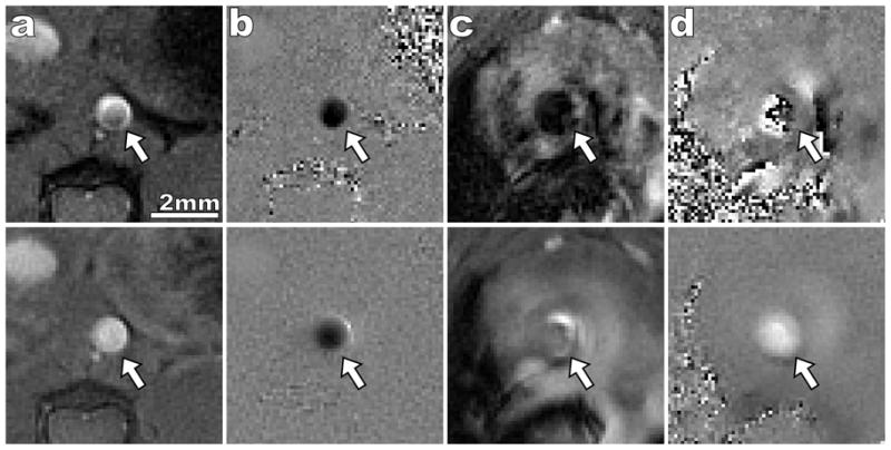
Comparison of rectilinear (top row) and spiral (bottom row) 2D cine PC sequence. The imaged portion of the aorta is indicated by a white arrow in all images. Systolic magnitude (a) and phase (b) images are shown for the thoracic aorta. Both sequences successfully capture flow within a straight region of the aorta. However, systolic magnitude (c) and phase (d) images of the ascending aorta illustrate the improved SNR and reduction in flow artifacts of the spiral sequence. When the rectilinear trajectory is used there is near complete signal loss within the aortic lumen which leads to speckle noise in the phase. Only minor signal loss occurs in the spiral image and a laminar velocity profile is seen within the lumen. Positive velocity corresponds to bright intensities in the phase image and negative velocity corresponds to dark intensities.
Figure 4.
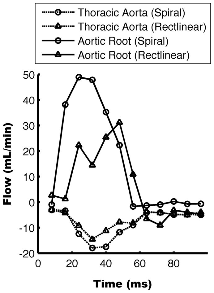
Flow rates measured with the two techniques from a representative mouse. Positive flow is in the caudal direction. Comparable flow profiles are measured with the rectilinear and spiral sequences within the thoracic aorta. However, peak flow is lost in the rectilinear sequence at the aortic root.
3D Spiral Cine PC
In Figure 5 the k-space trajectory errors are plotted as mean and standard deviation over all spiral interleafs. Maximal trajectory error was approximately 1/FOV, or one bin during gridding reconstruction. When reconstruction was performed ignoring trajectory errors and using the prescribed trajectory, edge streaking artifacts and signal inhomogeneities are visible (Figure 5b). When the measured trajectories are used during reconstruction, edge contrast and signal homogeneity are improved (Figure 5c).
Figure 5.
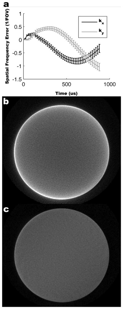
Measured k-space trajectories and reconstruction results in a cylindrical phantom. k-space trajectory errors as a function of time are shown for all spiral interleafs as mean ± standard deviation (a). In the lower panels the spiral reconstruction results are shown using the prescribed k-space trajectory (b) and measured k-space trajectory (c) (windowed identically). Using the measured trajectory yields improved edge definition and signal homogeneity.
Figure 6 shows a representative phase contrast dataset from a 24-week old ApoE−/− mouse. The aortic surface at systole is shown along with four reformats perpendicular to the aorta. Velocities are color coded according to through-plane velocity. As expected by geometry, higher velocities occur near the outer radius than the inner radius.
Figure 6.

Reformats through the mouse aortic arch. Sample aorta surface (top) shown with maximum intensity projections in the sagittal, axial, and coronal directions. Four slices are indicated by the blue rectangles and through plane velocities are shown in the bottom panels. The outer radius of the aorta is at the top of the lumen in all panels. An asymmetric distribution can be seen with higher velocities tending towards the outer radius as expected by fluid dynamics.
WSS Measurements
The asymmetrical distribution of velocities leads to significantly increased levels of WSS along the outer radius than the inner radius as illustrated in Figure 7. The instantaneous longitudinal and circumferential WSS waveforms are shown in Figure 8. During systole, the instantaneous longitudinal WSS is significantly larger along the outer radius than the inner radius (p<0.05). In contrast, the instantaneous circumferential WSS is significantly smaller along the outer radius than the inner radius (p<0.05). However, circumferential WSS was significantly smaller than longitudinal WSS magnitudes, and therefore had a smaller contribution to overall WSS magnitude. The inner radius had a higher OSI than the outer radius (0.14±0.01 v. 0.08±0.01; p<0.01) indicating increased WSS variability along the inner radius (Figure 8c).
Figure 7.
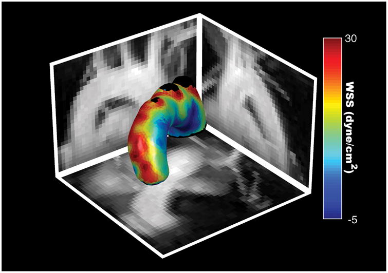
Time-averaged WSS magnitude map of a representative mouse shown with maximum intensity projections in the sagittal, axial, and coronal directions.
Figure 8.

Analysis of WSS cardiac cycle waveforms. (a) Longitudinal WSS was significantly higher along the outer radius of the aorta while (b) circumferential WSS was significantly higher along the inner radius of the aorta. Statistical significance was determined using two-way ANOVA (p<0.05) and is indicated by * at statistically significant cardiac phases. The increased variability of the WSS waveform is shown by a higher OSI along the inner radius than the outer radius (p<0.01).
In Figure 9 bulls eye plots are shown for the time averaged WSS and regional OSIs. Similar to the instantaneous WSS, the time-averaged longitudinal WSS was higher along the outer radius than the inner radius higher (18.86±1.27 dyne/cm2 v. 7.06±0.76 dyne/cm2; p<0.01) and the time-averaged circumferential WSS was higher along the inner radius than the outer radius (5.15±0.21 dyne/cm2 v. 2.04±0.68 dyne/cm2; p<0.01). Table 1 lists all the regional longitudinal WSS, circumferential WSS, and OSI values.
Figure 9.
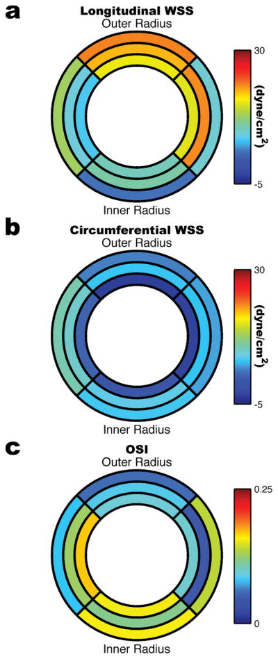
Bulls eye plots showing time-averaged (a) longitudinal WSS, (b) circumferential WSS, and (c) OSI in the 24-week old ApoE−/− mouse (n=5). The inner ring corresponds to the ascending region of the aortic arch, the middle ring to the top of the aortic arch, and the outer ring to the descending region of the aortic arch. The left and right quadrants correspond to the posterior and anterior sides of the arch respectively.
Table 1.
Regional values of WSS in ApoE−/− mice measured in dyne/cm2.
| Sector | τ̄l | τ̄c | OSI | |
|---|---|---|---|---|
| Ascending | Inner | 3.45±1.13 | 6.57±0.25 | 0.16±0.01 |
| Outer | 21.11±1.37 | 4.15±0.85 | 0.06±0.01 | |
| Anterior | 13.05±1.46 | 9.93±1.00 | 0.08±0.01 | |
| Posterior | 8.65±1.07 | 5.15±0.46 | 0.14±0.01 | |
| Top | Inner | 10.32±0.70 | 7.17±0.97 | 0.12±0.01 |
| Outer | 19.23±1.58 | 6.39±1.35 | 0.09±0.01 | |
| Anterior | 8.19±0.90 | 8.92±0.50 | 0.13±0.00 | |
| Posterior | 20.71±1.37 | 6.11±0.96 | 0.05±0.01 | |
| Descending | Inner | 9.62±0.97 | 0.75±0.75 | 0.16±0.01 |
| Outer | 16.33±1.32 | −2.90±0.69 | 0.10±0.01 | |
| Anterior | 6.64±0.69 | 2.38±0.84 | 0.17±0.01 | |
| Posterior | 16.02±1.28 | −2.65±0.54 | 0.10±0.01 | |
Discussion
The accurate measurement of velocity profiles in the mouse aorta necessitates the use of non-Cartesian trajectories to cope with the complex flow dynamics caused by fast moving spins moving through regions of high curvature. The favorable flow properties of spiral trajectories along with the short TE enabled velocity measurements throughout the mouse aortic arch. Comparison of a two-dimensional rectilinear and spiral PC sequence showed less flow artifact and higher signal intensity in regions of curved geometry and high flow for the spiral method. The spiral sequence was extended to three-dimensions to increase spatial coverage. As flow was no longer guaranteed to be orthogonal to the spiral trajectory axes, the three-dimensional scan used short spiral readouts to minimize misregistration artifacts. Even with the short spiral readouts, faster flows could cause misregistration artifacts. However, the centric read-outs minimize these artifacts and prevent interference with the velocity measurements near the vessel wall. This decrease in readout duration required the use of variable density scanning to perform the measurements within reasonable scan times.
WSS was directly calculated from the measured velocity gradients to investigate the relationship between hemodynamic forces and atheroprone regions. Longitudinal WSS was significantly smaller along the inner radius than the outer radius. Additionally, the WSS waveform was more oscillatory along the inner radius. This low, oscillatory WSS corresponds with regions traditionally predisposed to the development of atherosclerosis. Interestingly, the circumferential WSS was larger along the inner radius, likely due to the increased contribution of non-longitudinal flows.
The finite resolution of MRI leads to underestimation of the velocity gradient, and therefore leads to underestimation of WSS when direct measurement approaches are used (30). Although CFD models allow for resolution only limited by computation time, confounding factors such as compliance are difficult to measure and model within CFD leading to errors. The WSS magnitudes reported in this paper are smaller than reported previously in the aortic arch using CFD models, but are in agreement with published values using a direct measurement technique in the mouse thoracic aorta (32). The fact that WSS levels in atheroprone regions in the ApoE−/− mouse are above atheroprotective regions in humans suggests that it is not the absolute magnitude but the distribution and temporal pattern that are the determining factors in progression of atherosclerosis. Improving spatial resolution could decrease the underestimation of WSS in direct measurement techniques, however improvements in resolution would lead to increased scan times above the already hour long scan time. Methods such as parallel imaging (33) and compressed sensing (34) could be investigated to improve the spatial resolution without making scan times prohibitive. The low-pass nature of the median filter could also lead to a decrease in the calculated WSS value. However, as the median filter leaves velocity values unaltered in spatially monotonically increasing or decreasing regions the calculated WSS is expected to be affected less by a median filter than with other smoothing filters such as a spatial Gaussian filter.
The present study did not investigate the effect of the acceleration of the blood on the velocity measurements. Future work is necessary to determine what effect acceleration has on the velocity measurements and subsequent WSS calculations.
The echo times achieved with our spiral sequence led to large decreases in displacement artifacts compared to conventional rectilinear sequences; however, small displacement artifacts may remain using the present sequence and affect the WSS magnitude. As blood travels around the arch, a displacement artifact may result in faster moving blood being pulled towards the center of the arch. This displacement could lead to an underestimation of WSS along the outer radius and an overestimation of WSS along the inner radius. A future study using a pulse sequence with a further reduced echo time could be used to explore these effects.
Although the WSS calculation was limited to direct evaluation of the velocity gradient, future work should be aimed at incorporating the three-dimensional velocity measurements within CFD modeling. By not limiting CFD to only using flows at the inlets and outlets and instead extending the CFD models to include velocities throughout the modeled artery, effects of compliance can be more readily modeled. The union of more extensive velocity measurements along with CFD modeling may lead to improved estimates over either direct measurement or CFD approaches alone.
The described technique enables a tool for directly probing the relationship between WSS and atherosclerosis in mouse models. The direct measurement of WSS in combination with the assessment of protein expression may lead to increased understanding of the molecular factors involved in atherosclerosis and the effect WSS has on the disease process.
Acknowledgments
This research was funded by an AHA Pre-Doctoral Fellowship 0715233U and through NIH NHLBI HL082836-01, NIH NIBIB R01 EB 001763 and NIH NHLBI RO1 HL079110.
References
- 1.Ross R. Atherosclerosis -- An Inflammatory Disease. N Engl J Med. 1999;340(2):115–126. doi: 10.1056/NEJM199901143400207. [DOI] [PubMed] [Google Scholar]
- 2.Hansson GK. Inflammation, Atherosclerosis, and Coronary Artery Disease. N Engl J Med. 2005;352(16):1685–1695. doi: 10.1056/NEJMra043430. [DOI] [PubMed] [Google Scholar]
- 3.Cunningham KS, Gotlieb AI. The role of shear stress in the pathogenesis of atherosclerosis. Lab Invest. 2004;85(1):9–23. doi: 10.1038/labinvest.3700215. [DOI] [PubMed] [Google Scholar]
- 4.Reneman RS, Arts T, Hoeks APG. Wall Shear Stress -- an Important Determinant of Endothelial Cell Function and Structure -- in the Arterial System in vivo. J Vasc Res. 2006;43(3):251–269. doi: 10.1159/000091648. [DOI] [PubMed] [Google Scholar]
- 5.Nakashima Y, Plump AS, Raines EW, Breslow JL, Ross R. ApoE-deficient mice develop lesions of all phases of atherosclerosis throughout the arterial tree. Arterioscler Thromb Vasc Biol. 1994;14:133–140. doi: 10.1161/01.atv.14.1.133. [DOI] [PubMed] [Google Scholar]
- 6.Cheng C, Tempel D, van Haperen R, van der Baan A, Grosveld F, Daemen MJAP, Krams R, de Crom R. Atherosclerotic Lesion Size and Vulnerability Are Determined by Patterns of Fluid Shear Stress. Circulation. 2006;113(23):2744–2753. doi: 10.1161/CIRCULATIONAHA.105.590018. [DOI] [PubMed] [Google Scholar]
- 7.Zadelaar S, Kleemann R, Verschuren L, de Vries-Van der Weij J, van der Hoorn J, Princen HM, Kooistra T. Mouse Models for Atherosclerosis and Pharmaceutical Modifiers. Arterioscler Thromb Vasc Biol. 2007;27(8):1706–1721. doi: 10.1161/ATVBAHA.107.142570. [DOI] [PubMed] [Google Scholar]
- 8.Cheng C, van Haperen R, de Waard M, van Damme LCA, Tempel D, Hanemaaijer L, van Cappellen GWA, Bos J, Slager CJ, Duncker DJ, van der Steen AFW, de Crom R, Krams R. Shear stress affects the intracellular distribution of eNOS: direct demonstration by a novel in vivo technique. Blood. 2005;106(12):3691–3698. doi: 10.1182/blood-2005-06-2326. [DOI] [PubMed] [Google Scholar]
- 9.Fabrizio Rodella L, Bonomini F, Rezzani R, Tengattini S, Hayek T, Aviram M, Keidar S, Coleman R, Bianchi R. Atherosclerosis and the protective role played by different proteins in apolipoprotein E-deficient mice. Acta Histochem. 2007;109(1):45–51. doi: 10.1016/j.acthis.2006.08.002. [DOI] [PubMed] [Google Scholar]
- 10.Suo J, Ferrara DE, Sorescu D, Guldberg RE, Taylor WR, Giddens DP. Hemodynamic Shear Stresses in Mouse Aortas: Implications for Atherogenesis. Arterioscler Thromb Vasc Biol. 2007;27(2):346–351. doi: 10.1161/01.ATV.0000253492.45717.46. [DOI] [PubMed] [Google Scholar]
- 11.Feintuch A, Ruengsakulrach P, Lin A, Zhang J, Zhou Y-Q, Bishop J, Davidson L, Courtman D, Foster FS, Steinman DA, Henkelman RM, Ethier CR. Hemodynamics in the mouse aortic arch as assessed by MRI, ultrasound, and numerical modeling. Am J Physiol-Heart C. 2007;292(2):H884–892. doi: 10.1152/ajpheart.00796.2006. [DOI] [PubMed] [Google Scholar]
- 12.Greve JM, Les AS, Tang BT, Draney Blomme MT, Wilson NM, Dalman RL, Pelc NJ, Taylor CA. Allometric scaling of wall shear stress from mice to humans: quantification using cine phase-contrast MRI and computational fluid dynamics. Am J Physiol-Heart C. 2006;291(4):H1700–1708. doi: 10.1152/ajpheart.00274.2006. [DOI] [PubMed] [Google Scholar]
- 13.Gelfand BD, Epstein FH, Blackman BR. Spatial and spectral heterogeneity of time-varying shear stress profiles in the carotid bifurcation by phase-contrast MRI. J Magn Reson Imaging. 2006;24(6):1386–1392. doi: 10.1002/jmri.20765. [DOI] [PubMed] [Google Scholar]
- 14.Nayak KS, Hu BS, Nishimura DG. Rapid quantitation of high-speed flow jets. Magn Reson Med. 2003;50(2):366–372. doi: 10.1002/mrm.10538. [DOI] [PubMed] [Google Scholar]
- 15.Nishimura DG, Irarrazabal P, Meyer CH. A Velocity k-Space Analysis of Flow Effects in Echo-Planar and Spiral Imaging. Magn Reson Med. 1995;33(4):549–556. doi: 10.1002/mrm.1910330414. [DOI] [PubMed] [Google Scholar]
- 16.Meyer CH, Hu BS, Nishimura DG, Macovski A. Fast Spiral Coronary Artery Imaging. Magn Reson Med. 1992;28(2):202–213. doi: 10.1002/mrm.1910280204. [DOI] [PubMed] [Google Scholar]
- 17.Takahashi A, Li T-Q, Stodkilde-Jorgensen H. A Pulse Sequence for Flow Evaluation Based on Self-Refocused RF and Interleaved Spiral Readout. J Magn Reson. 1997;126(1):127–132. doi: 10.1006/jmre.1997.1128. [DOI] [PubMed] [Google Scholar]
- 18.Pike GB, Meyer CH, Brosnan TJ, Pelc NJ. Magnetic resonance velocity imaging using a fast spiral phase contrast sequence. Magn Reson Med. 1994;32(4):476–483. doi: 10.1002/mrm.1910320409. [DOI] [PubMed] [Google Scholar]
- 19.Irarrazabal P, Meyer CH, Nishimura DG, Macovski A. Inhomogeneity correction using an estimated linear field map. Magn Reson Med. 1996;35(2):278–282. doi: 10.1002/mrm.1910350221. [DOI] [PubMed] [Google Scholar]
- 20.Pelc NJ, Bernstein MA, Shimakawa A, Glover GH. Encoding strategies for three-direction phase-contrast MR imaging of flow. J Magn Reson Imaging. 1991;1(4):405–413. doi: 10.1002/jmri.1880010404. [DOI] [PubMed] [Google Scholar]
- 21.Gatehouse PD, Firmin DN. Flow distortion and signal loss in spiral imaging. Magn Reson Med. 1999;41(5):1023–1031. doi: 10.1002/(sici)1522-2594(199905)41:5<1023::aid-mrm22>3.0.co;2-1. [DOI] [PubMed] [Google Scholar]
- 22.Spielman DM, Pauly JM, Meyer CH. Magnetic resonance fluoroscopy using spirals with variable sampling densities. Magn Reson Med. 1995;34(3):388–394. doi: 10.1002/mrm.1910340316. [DOI] [PubMed] [Google Scholar]
- 23.Zhang Y, Hetherington HP, Stokely EM, Mason GF, Twieg DB. A novel k-space trajectory measurement technique. Magn Reson Med. 1998;39(6):999–1004. doi: 10.1002/mrm.1910390618. [DOI] [PubMed] [Google Scholar]
- 24.Duyn JH, Yang Y, Frank JA, van der Veen JW. Simple Correction Method for k-Space Trajectory Deviations in MRI. J Magn Reson. 1998;132(1):150–153. doi: 10.1006/jmre.1998.1396. [DOI] [PubMed] [Google Scholar]
- 25.Ghiglia DC, Pritt MD. Two-Dimensional Phase Unwrapping: Theory, Algorithms, and Software. New York, NY: John Wiley & Sons, Inc; 1998. [Google Scholar]
- 26.Lingamneni A, Hardy PA, Powell KA, Pelc NJ, White RD. Validation of cine phase-contrast MR imaging for motion analysis. J Magn Reson Imaging. 1995;5(3):331–338. doi: 10.1002/jmri.1880050318. [DOI] [PubMed] [Google Scholar]
- 27.Janiczek RL, Epstein FH, Acton ST. Automatic Segmentation of 3D Phase Contrast MRI using Velocity Guided Gradient Vector Flow. Proceedings of the 17th Annual Meeting of ISMRM; Honolulu, Hawaii, USA. 2009. p. 3824. [Google Scholar]
- 28.Bühler K, Felkel P, Cruz AL. Geometric Methods for Vessel Visualization and Quantification - A Survey. In: Brunnett G, Hamann B, Müller H, Linsen L, editors. Geometric Modeling for Scientific Visualization. Berlin: Springer; 2004. pp. 399–420. [Google Scholar]
- 29.Bouix S, Siddiqi K, Tannenbaum A. Flux driven automatic centerline extraction. Med Image Anal. 2005;9(3):209–221. doi: 10.1016/j.media.2004.06.026. [DOI] [PubMed] [Google Scholar]
- 30.Stalder AF, Russe MF, Frydrychowicz A, Bock J, Hennig J, Markl M. Quantitative 2D and 3D phase contrast MRI: Optimized analysis of blood flow and vessel wall parameters. Magn Reson Med. 2008;60(5):1218–1231. doi: 10.1002/mrm.21778. [DOI] [PubMed] [Google Scholar]
- 31.He X, Ku DN. Pulsatile Flow in the Human Left Coronary Artery Bifurcation: Average Conditions. J Biomech Eng. 1996;118(1):74–82. doi: 10.1115/1.2795948. [DOI] [PubMed] [Google Scholar]
- 32.Zhao X, Pratt R, Wansapura J. Quantification of aortic compliance in mice using radial phase contrast MRI. J Magn Reson Imaging. 2009;30(2):286–291. doi: 10.1002/jmri.21846. [DOI] [PubMed] [Google Scholar]
- 33.Meyer CH, Hu P. Spiral Parallel Magnetic Resonance Imaging. Engineering in Medicine and Biology Society; New York, New York, USA: 2006. pp. 369–371. [DOI] [PubMed] [Google Scholar]
- 34.Lustig M, Donoho D, Pauly JM. Sparse MRI: The application of compressed sensing for rapid MR imaging. Magn Reson Med. 2007;58(6):1182–1195. doi: 10.1002/mrm.21391. [DOI] [PubMed] [Google Scholar]