Maps of interaural time difference in the chicken’s brainstem nucleus laminaris

Abstract

Animals, including humans, use interaural time differences (ITDs) that arise from different sound path lengths to the two ears as a cue of horizontal sound source location. The nature of the neural code for ITD is still controversial. Current models differentiate between two population codes: either a map-like rate-place code of ITD along an array of neurons, consistent with a large body of data in the barn owl, or a population rate code, consistent with data from small mammals. Recently, it was proposed that these different codes reflect optimal coding strategies that depend on head size and sound frequency. The chicken makes an excellent test case of this proposal because its physical pre-requisites are similar to small mammals, yet it shares a more recent common ancestry with the owl. We show here that, like in the barn owl, the brainstem nucleus laminaris in mature chickens displayed the major features of a place code of ITD. ITD was topographically represented in the maximal responses of neurons along each isofrequency band, covering approximately the contralateral acoustic hemisphere. Furthermore, the represented ITD range appeared to change with frequency, consistent with a pressure gradient receiver mechanism in the avian middle ear. At very low frequencies, below400 Hz, maximal neural responses were symmetrically distributed around zero ITD and it remained unclear whether there was a topographic representation. These findings do not agree with the above predictions for optimal coding and thus revive the discussion as to what determines the neural coding strategies for ITDs.

1 Introduction

Accurate coding of temporal information has direct behavioral relevance for the computation of sound source location. Birds and mammals show exquisite sensitivity to interaural time differences (ITDs): when sound comes from one side of the body, it reaches one ear before the other. The brain uses these ITDs to compute sound location in the horizontal (azimuthal) plane (Konishi 2003; Yin 2002).

There is general agreement that the basic sensitivity for ITD and binaural correlation arises through a cross-correlation like comparison of inputs to the two ears (Batra and Yin 2004; Joris and Yin 2007; Yin et al. 1987). The cross correlator neurons act as coincidence detectors (reviews in Grothe 2003; Konishi 2003; Yin 2002). The coincidence detection is performed separately and in parallel in many narrowly tuned frequency channels. The sound waveform is encoded by phase-locked neural discharges in the auditory nerve, i.e. by a precise correlation between the phase of the stimulus and the firing of spikes. Coincidence detection between such inputs from each ear gives rise to a discharge pattern that varies cyclically as a function of interaural phase difference, showing a maximum when both inputs are in phase and a minimum when they are 180° out of phase. Thus, sensitivity to interaural phase differences (IPDs) is created. IPD is a relative measure of time and, knowing the stimulus period, can be translated into absolute ITD. In fact, within each narrowly tuned frequency channel, IPD and ITD are interchangeable. ITD is the physical cue to the azimuthal position of a sound source. A current controversy centers on the question of how the coding of a range of ITDs enables the nervous system to precisely localize sound sources along the azimuthal plane.

In principle, an array of coincidence detectors could be set up, situated along interdigitating or counter-current delay line inputs from each ear. In such a circuit, the delay lines introduce successively greater input delays to the coincidence detectors they contact serially. In consequence, each individual coincidence detector fires maximally at the phase difference between its inputs that exactly compensates for the conduction delay introduced at its place. Such a circuit, generating a place map of interaural phase difference at each frequency is well known as the place-code model or Jeffress model, after Jeffress (1948). However, the task of ITD coding is affected by both head size and the ability to phase lock. The sharpness of ITD selectivity of the individual coincidence detectors increases for neurons with higher characteristic frequency because their temporal precision is greater. For example, the spikes of an auditory neuron phase-locking to a 5kHz stimulus (with a period of 200 μs) show a temporal dispersion of about ±40 μs around the preferred phase; for a neuron phase-locking to 1 kHz (with a period of 1 ms) the temporal dispersion is typically ±100 μs (Köppl 1997). In coincidence detector neurons using such inputs, this results in correspondingly steeper slopes for the 5 kHz and shallower slopes for the 1 kHz ITD selectivity curves (Batra and Yin 2004). Animals with smaller heads that naturally experience a smaller ITD range therefore have less precise information available at equivalent frequencies than animals with larger heads.

Animals with smaller heads also do not have the option of simply using higher frequencies. As the above example illustrates, phase-locking is a process that demands increasing temporal precision in spike generation with increasing frequency. Due to the biophysical limitations of the cell membranes involved, phase-locking faces a clear upper frequency limit. For the auditory neurons providing the input to the coincidence detector circuits discussed here, this upper limit varies between 3 and 10kHz in different species (review in Köppl 1997).

The basic problem of the interaction between head size and the frequency range available for creating the neural code of ITD was formalized in a model of IPD representation (Harper and McAlpine 2004). Assuming that the ITDs an animal naturally encounters should be coded with maximal accuracy, Harper and McAlpine (2004) argued that the neural representation of IPD within the population of the first binaural coincidence detectors should conform to either one of two distinct strategies, depending on head size and frequency range. One is a homogeneous distribution of the maxima of their selectivity curves (hereafter called best IPD), collectively covering the physiological ITD range of the animal within each frequency band. Although the model does not address the question as to how the distribution is achieved, such a distribution is consistent with the Jeffress model and an orderly representation of best IPDs along input delay lines. The second strategy of ITD coding is characterized by a non-homogeneous distribution of best IPD, with distinct subpopulations of neurons within each frequency band. The best IPDs of each population fall within a narrow range and often outside the physiological range of the animal. Instead of the maxima, the slopes of the IPD-selectivity curves cover the physiological range, and each slope covers most of this range. Various terms and variations have been suggested for this broad category of models in the past, summarized as Left–Right Count-Comparison models by Colburn and Kulkarni (2005). Here, the term two-channel model will be used, emphasizing the fact that all the coincidence detectors of each brainstem hemisphere together are believed to comprise one channel (or population). The relative excitation in the two channels from the two hemispheres is assumed to be read out as a correlate of ITD and thus as azimuthal sound source location (review in Palmer 2004).

Experimental evidence for both types of models of ITD coding exists. As has been reviewed by many authors (e.g. Konishi 2003), all of the characteristics of the Jeffress model appear fulfilled in the relevant brainstem nucleus (Nucleus laminaris, NL) of the barn owl, at least within the frequency range that has been extensively studied (above 3 kHz; Carr and Konishi 1990; Pena et al. 1996). Experimental data from the equivalent brainstem nucleus (medial superior olive, MSO) in the gerbil provide the clearest support for the two-channel model (Brand et al. 2002). In addition, a likely neural mechanism has been revealed in the gerbil for creating the unique distribution of best IPDs. It relies on additional phase-locked inhibitory inputs to the coincidence detector (MSO) neurons and does not require input delay lines (reviewed in Grothe 2003). However, data from different mammalian species are often ambiguous and their interpretation in support for the Jeffress model on the one hand or the two-channel model on the other is intensely controversial (recent summaries in Joris and Yin 2007; McAlpine 2005; Palmer 2004).

A virtue of the optimal coding scheme suggested by Harper and McAlpine (2004) is that it makes clear predictions for specific examples of head sizes and frequencies about which coding strategy should be optimal and thus allows for experimental testing. As a general rule, a Jeffress-like code and homogeneous representation of best IPDs is optimal at frequencies high enough so that the head’s ITD range exceeds ±0.5 cycles, while one or two channels with discrete populations of best IPD are optimal at frequencies below that. The barn owl and the gerbil were put forward as examples where experimental data clearly fit those predictions, however, this has recently been challenged for the low-frequency range of the owl (Wagner et al. 2007).

The key prediction of Jeffress’ model, a topographic map of best ITD in the MSO or NL, has not been experimentally addressed recently. In 1990, Carr and Konishi used physiological and anatomical techniques to show that axonal delay lines form maps of ITD in the NL of the barn owl. In the cat, two studies provided anatomical evidence for axonal delay lines in the contralateral afferents (Beckius et al. 1999; Smith et al. 1993), while Yin and Chan (1990) showed a correlation between best delay and rostrocaudal position in the MSO. However, the owl has been challenged as a highly specialized and potentially untypical case (e.g. McAlpine 2005) and the evidence in the cat is not conclusive (Joris and Yin 2007).

We have therefore examined this key prediction in the chicken, an unspecialized bird with a small range of physiological ITDs (Hyson et al. 1994) and a relatively low range of frequencies of phase-locking (Salvi et al. 1992), both similar to the values in the gerbil. Harper and McAlpine’s (2004) optimal coding scheme predicts ITD coding in discrete channels for frequencies up to 3 kHz, i.e., up to the limit of phase-locking. However, anatomical studies show that the chicken Nucleus magnocellularis (NM) projects in a delay-line pattern to NL (Parks and Rubel 1975; Young and Rubel 1983) and appropriate conduction delays have been measured in brain-slice preparations of this circuit (Overholt et al. 1992). This suggests a map-like representation of a range of IPDs, inconsistent with the prediction of a uniform population of neurons on each side of the brainstem. However, it is unknown whether those delay lines determine the responses of NL neurons in the mature chicken in vivo and if so, what range of IPDs they cover. We have carried out in vivo recordings of NL activity, combined with histological verification of recording sites. We show that the NL contains a systematic, gradual representation of the animal’s ITD range. This and a host of monaural and binaural response properties investigated are entirely consistent with the Jeffress model.

2 Materials and methods

Experiments were carried out on 22 chickens aged between 17 and 41 days after hatching. Animal husbandry and experimental protocols were approved by the Regierung von Oberbayern, Germany (AZ 209.1/211-2531-56/04) for a first series of experiments and by the University of Sydney, NSW, Australia (Animal Ethics Committee Approval No. K03/1-2007/3/4526) for a subsequent series.

2.1 Anesthesia and surgery

Anesthesia was induced by intramuscular injections of 20 mg/kg ketamine hydrochloride (Ketavet by Pharmacia GmbH, Erlangen, Germany or Ketamine by Parnell Laboratories, Alexandria, NSW, Australia) and 3mg/kg xylazine (Rompun by Bayer Vital GmbH, Leverkusen, Germany or Ilium Xylazil-20 by Troy Laboratories, Smithfield, NSW, Australia) and maintained with supplementary doses as necessary until switching to isoflurane (see below). In addition, a subset of animals received approximately 20 mg/kg metamizol-sodium (Vetalgin by Intervet GmbH, Unterschleissheim, Germany) every 3–4 h, as required by German authorities. Body temperature was maintained at 41°C by a heating blanket wrapped around the animal and feedback-controlled by a cloacal temperature probe. An EKG recording via needle electrodes placed in the muscles of the right wing and left leg was constantly monitored. The trachea was cut and intubated. After opening the abdominal air sac just below the ribs, a constant, humidified gas flow of 150–400 ml/min (approximately 1ml/g body weight)was connected to the tracheal tube. Spontaneous breathing ceased under these conditions. The gas was either carbogen or pure oxygen, mixed with 0.8–1.5% isoflurane. The head was held in a constant position and the skull was opened to expose the cerebellum. The medial sinus was ligated, and most of the cerebellum aspirated to expose the dorsal surface of the brainstem.

2.2 Recordings and iontophoresis

Thin-walled glass microelectrodes were filled with 5% neurobiotin in 2MK-acetate, positioned above the relevant brainstem area under visual control and then advanced remotely with a piezo device (Inchworm 700, Burleigh, Fishers, NY). Responses to acoustic stimuli were monitored continuously until we were confident that the electrode was within the cellular layer of NL. Responses were amplified (Intra 767, World Precision Instruments, Sarasota); the amplified signal was usually high-pass filtered at 300 Hz, except for the extreme low-frequency recordings, (module PC1, Tucker-Davis Technologies (TDT), Alachua) and fed in parallel to an A/D converter (TDT DD1) and a threshold discriminator (TDT SD1) with subsequent event counter (TDT ET1). As single-unit spike recordings could only rarely be achieved, most of the recordings were of the neurophonic potential, a sinusoidal evoked potential reflecting the frequency of a pure-tone stimulus. For neurophonic recordings, the TTL trigger threshold was subjectively adjusted for optimal signal-to-noise ratio. Both the analog and the TTL signal could be stored by custom-written software (xdphys, California Institute of Technology).

At selected recording sites, neurobiotin was deposited iontophoretically, usually by passing 250nA of positive direct current for 10mins.

2.3 Stimulus generation and presentation

Chickens were placed in a sound-attenuating chamber for all measurements. Closed, custom-made sound systems, containing small earphones (Sony MDR-E818LP) and miniature microphones (Knowles EM 3068), were placed at the entrance of both ear canals, but not tightly sealed. The sound systems were calibrated individually for both amplitude and phase before the recordings.

Stimuli were generated separately for the two ears by custom-written software (xdphys, Caltech), using a TDT AP2 signal processing board. Both channels were then fed to the earphones via D/A converters (TDT DD1), anti-aliasing filters (TDT FT6-2) and attenuators (TDT PA4). Stimuli were tone bursts of 50ms duration (including 5ms linear ramps), presented at a rate of 5s⁻¹, or clicks, presented at a rate of 10s⁻¹.

2.4 Data collection and analysis

2.4.1 Monaural tuning curves, characteristic frequency (CF) and threshold

Monaural frequency-versus-level responses for both ipsi- and contralateral stimulation were recorded first, by presenting tones from a matrix of frequencies and sound pressure levels in random sequence, repeated three times. Monaural tuning curves were derived from these as described in Köppl and Carr (2003), using the recorded TTL signal in all cases. The mean of their CFs and thresholds were taken as the CF and threshold of the recording site.

2.4.2 Monaural click responses

Responses to 500 repetitions of monaurally presented clicks were recorded. For single-unit recordings, a peristimulus-time histogram (PSTH) with a bin width of 0.02ms was calculated, using the TTL signal. Latency was defined as the earlier of the first two consecutive bins exceeding the tallest bin in a 10ms interval preceeding the stimulus. For neurophonic recordings, the averaged analog response waveform was analyzed as described in Wagner et al. (2005) for NL neurophonic data from the barn owl. Briefly, the waveform was high-pass filtered to exclude components below the CF and subsequently fitted with a gammatone function. This type of analysis was well applicable to chicken neurophonic click responses, too, if the cut-off frequencies of the filter functions were adjusted to the lower frequency range of the chicken. Fitted waveforms of ipsi- and contralateral responses were then superimposed. The median difference between 2 and 4 consecutive maxima and minima was taken as the difference in response latency, with positive values indicating contralateral leading.

2.4.3 Monaural phase responses

Responses to 100 repetitions of monaurally presented tones at a frequency close to the CF, and a level of 40–60 dB SPL, corresponding to an average of 16 dB above threshold, were recorded. Using the TTL signal in all cases, mean phase and vector strength (VS) were derived from these according to Goldberg and Brown (1969). Only VS values with a significance level of 0.01 or below were accepted. The difference between the mean phases for ipsi- and contralateral stimulation were then calculated as a predictor of best IPD, using the click responses as a guideline as to which side was leading.

2.4.4 Best IPD, characteristic delay (CD) and characteristic phase (CP)

Sensitivity for ITD was tested with tones presented binaurally with various time disparities. ITD was usually varied within ±1 stimulus period, in steps no larger than one-tenth of the period. Stimulus level was the same as for monaural phase responses (40–60 dB SPL or, on average, 16 dB above monaural thresholds); Usually 10 stimulus repetitions were presented at each ITD. As a rule, for single units, the TTL signal, i.e., spike rate, was used for further analysis, for neurophonic recordings the amplitude of the analog waveform was used. The only exceptions to this were data from the earliest experiments (9 of 44 neurophonic sites), where the analog signal was not saved. For these neurophonic data, TTL counts exceeding a subjectively set threshold were also used. We found later, comparing both types of analysis for neurophonic recordings, that the results did not differ systematically, but that the neurophonic amplitude provided a better signal-to-noise ratio. The frequencies at which ITD sensitivity was tested always included the CF previously determined from monaural tuning curves. Because of the well-known sharpness of tuning in the lower auditory centres of birds, the range of frequencies over which responses could be obtained was limited. We developed empirical criteria for the acceptance or rejection of data at particular frequencies for further analysis. For single units, the mean spike rate and standard deviation was determined for each ITD and an index of modulation derived by calculating the difference between minimal and maximal mean rate and dividing it by the maximal standard deviation observed. Data were discarded if this index was below 1.5. For neurophonic recordings, the averaged analog response waveform at each ITD was fitted with a cosine function at the stimulus frequency. The amplitude of this fit was then divided by: standard deviation of the averaged waveform *√2. The value of this index is 1 if the waveform is identical to the fitted cosine and becomes zero if the waveform contains no stimulus frequency component. Data were discarded if this index remained below 0.7 at all ITDs tested. Acceptable data according to these criteria usually fell within a range of 0.2–0.5 octaves around CF (median 0.33 octaves). The neurophonic amplitudes or, for single units, the spike rate, as a function of lTD were then fitted with a cosine function at the respective stimulus frequency (Viete et al. 1997) to determine best IPD, defined as the peak closest to zero IPD. In cases where the minimum fell close to zero IPD and it was thus ambiguous which peak defined the best IPD, click responses and the CD (see next) were used to resolve the laterality. Finally, a linear regression of best IPD as a function of frequency was calculated, the slope of which corresponds to the CD and the y-intercept to the CP (Yin and Kuwada 1983).

2.4.5 Histology

Chickens were fixed by cardiovascular perfusion with 4% buffered paraformaldehyde, the brains were extracted, cryo-protected by infiltration with 30% sucrose and cross-sectioned on a cryostat. Neurobiotin was visualized using standard ABC (Vector Laboratories, Burlingame, CA) and diaminobenzidine protocols on floating sections. Finally, the sections were serially mounted and counterstained with cresyl violet.

All sections containing NL were identified and the position of NL’s medial edge relative to the midline was measured in each. The linear extent of the nucleus was then measured along the neuron chain, regardless of its orientation within the section, as well as the position of any neurobiotin label along that dimension. These data were then used to construct a flat surface view of NL and determine the position of label in normalized coordinates, with reference to the total mediolateral and rostrocaudal extent of NL. Note that the mediolateral dimension in this scheme represents an artificially flattened view of NL and is not identical to the brain’s mediolateral axis. This is different to the surface projection of NL used by Rubel and Parks (1975). All measurements were carried out with the use of image analysis software (AnalySIS by Soft Imaging Software, Münster, Germany).

3 Results

We report a total of 43 neurophonic recordings, 3 extracellular multi-unit recordings, 14 extracellular single-unit spike recordings and 4 intracellular recordings from the NL of the chicken in vivo. Thirty-four of these recording sites were histologically located within the cellular layer of NL by neurobiotin labeling. The neurophonic is a sinusoidal evoked potential reflecting the frequency of the pure-tone stimulus (Schwarz 1992; Sullivan and Konishi 1986). It is more easily and stably recorded than single units, but its precise origin has not been explored. We suggest that it predominantly originates from the NL neurons, for the following reasons. In the chicken, the maximal amplitude of the neurophonic potential is very localized and falls sharply with distance from the cellular monolayer of NL (Schwarz 1992). We were able to confirm this well-localized nature. Using high-impedance electrodes (typically between 10 and 25 MΩ), the location of maximal neurophonic amplitude could usually be judged to within 50 μm by audiovisual criteria, and care was taken to position the electrode at this maximum before recording and subsequent iontophoresis of neurobiotin. In addition, we observed that the neurophonic thresholds to ipsi- and contralateral stimulation were most similar at that point and provided another useful criterion. In many cases, 1–3 labeled cell bodies were later seen in the histological sections, confirming that the electrode was in the neuron layer. In the rare cases of intracellular recordings (indicated by a sudden jump of the recorded DC potential to between −20 and −50 mV) the response appeared like a magnified neurophonic with either small or no spikes superimposed on the sinusoidal waveform. For direct comparison, we have a brief intracellular recording from an NL neuron, obtained within 25 μm of a neurophonic recording with the same electrode. In addition, there is one case of an extracellular spike recording and, after the loss of spikes, the corresponding neurophonic recording at the same site. In both cases, the ITD selectivities of the neurophonic potential and the corresponding single unit were very similar (Fig. 1).

Fig. 1.

ITD selectivities of the neurophonic potential and of single cells at the same site were identical. a Extracellular single-unit recording (black line) and neurophonic recording (gray line), obtained after the loss of spikes at the same site, without moving the electrode. Because in this early experiment no analog version was recorded for the neurophonic, its TTL signal count is shown as the response parameter (many later comparisons of analog vs. TTL analysis of the same data set showed no systematic difference, but the signal-to-noise ratio was generally better in the analog version). b Intracellular recording from an NL neuron (black line), obtained within 25 μm of a neurophonic recording (gray line) with the same electrode. Here, for both cases the amplitude of the analog signal is shown as the response parameter, because no spikes were evident in the intracellular record. In both panels, values above the graphs give the best ITDs derived from cosine fits to the data shown (positive numbers indicate contralateral leading)

3.1 Range of characteristic frequencies, thresholds and their binaural match

Characteristic frequencies (CF) ranged from 80 to 3,500 Hz. Figure 2 shows the distributions of mean CFs and thresholds, as well the differences between the monaurally determined measures for each recording site. Most of our data were obtained between 1 and 2.5 kHz CF, as this region of NL was most easily accessible. There was no systematic mismatch between the monaural CFs or the monaural thresholds of a particular recording site. Median differences were 0 Hz for the paired CFs (interquartile range −75 to +100 Hz) and 1 dB for the thresholds (interquartile range −3.5 to +5 dB). Wilcoxon tests showed that there were no significant differences between the paired samples (p = 0.84 for CFs, p = 0.65 for thresholds).

Fig. 2.

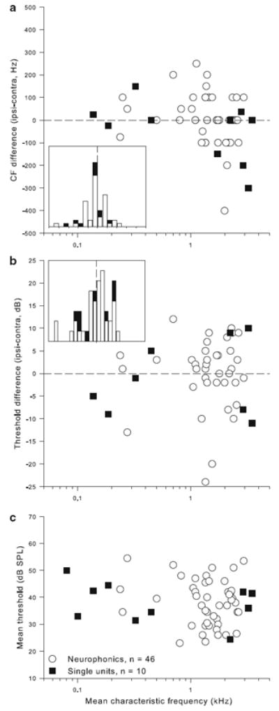
Monaural characteristic frequencies and thresholds matched on average. a Difference between monaurally determined CFs as a function of mean CF, for all neurophonic recording sites (open circles) and single units (filled squares). The inset shows a bar histogram of the same data, in 50 Hz bins, with 0 Hz difference emphasized by the dashed line. b Difference between monaurally determined thresholds, shown in the same format as a. The bin width in the insert is 2 dB. c Mean threshold as a function of mean CF

3.2 Monaural click and phase responses

Monaural click responses of neurophonic recordings usually showed a clear oscillatory component of a frequency close to CF. Comparing the responses to ispi- and contralateral clicks provided an unambiguous measure of laterality and a prediction for best ITD (Fig. 3a). In a minority of cases (7 neurophonic recordings), the response waveforms could not be unambiguously matched because of significant differences in shape; these were excluded from further analysis. Formulti- or single-unit recordings, PSTH histograms of spike responses to monaural click stimuli were used (Fig. 3b, c). With one exception, all recording sites analysed (n = 41) showed either an ipsilaterally leading click response or equal response latencies to both sides. Ipsilateral lead times ranged up to 1,020 μs, but mostly fell below 400 μs (see also later Fig. 12). The one exception was a low-frequency single unit (CF 138 Hz), responding 160 μs earlier to the contralateral click.

Fig. 3.

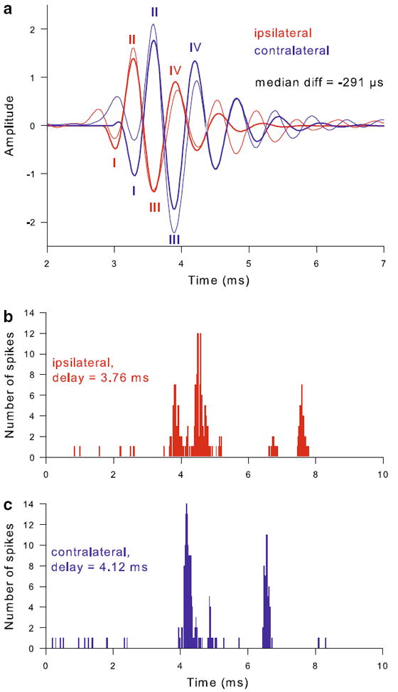
Monaural click responses unambiguously indicated response laterality. a Response waveforms to monaural click stimulation of a neurophonic recording with CF = 1.75 kHz. Thin lines show the averaged waveform in response to 500 condensation clicks; thick lines represent the gammatone fit to the high-pass filtered response, which was used to determine the latency of the initial four minima and maxima (labeled I to IV, see Methods for details). The ipsilateral response is shown in red, the contralateral one in blue. The median latency difference between ipsi- and contralateral response minima and maxima was −291 μs. b, c PSTH histograms for responses to ipsi- (b) and contralateral (c) clicks of a single unit of CF = 450 Hz. The bin width is 0.02 ms. The latency difference was −360 μs in this case

Fig. 12.

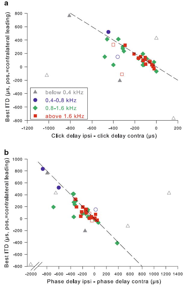
Monaural responses predicted best ITD at most frequencies. Best ITD as a function of the difference between monaural click response delays (panel a) or the difference between monaural phase response delays (panel b). Note that all values are given according to a uniform sign convention (positive = contralateral leading); therefore best ITD is ideally expected to be of opposite sign to the monaural difference, as indicated by the dashed reference lines. Data at CFs above 0.4 kHz showed a tight correlation between their binaural best ITD and the difference predicted by the monaural responses. At lower CFs, the predicted and actual ITD did not match as well

All recording sites tested (n = 53) displayed significant phase locking to monaural pure-tone stimuli near CF. Vector strengths for ipsi- and contralateral stimulation were generally similar (no median difference) and decreased with increasing frequency (Fig. 4). The difference between the preferred response phases to ipsi- and contralateral stimulation was used to predict the preferred ITD (see below), using the click responses and/or CD to resolve phase ambiguity.

Fig. 4.

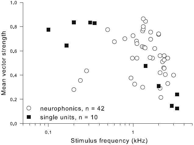
Vector strength of phase locking declined with increasing frequency. Mean monaural vector strength is plotted as a function of stimulus frequency

3.3 Range of best IPDs and ITDs

All NL recordings showed sensitivity for ITD, in the form of cyclic changes of neurophonic amplitude or of spike rate with variations in ITD. The cycle period corresponded to the period of the stimulus, which was chosen to be close to the CF. Best IPDs ranged from −0.57 to +0.58 cycles (Fig. 5b; median +0.131; positive values indicating contralateral leading, negative values indicating ipsilateral leading). Note that best IPDs beyond ±0.5 cycles could and did occur because monaural click responses and/or the CD were used as the ultimate indicators of laterality. For example, if the peak of the IPD function closest to zero fell at −0.445 cycles, but the click responses indicated a shorter delay for the ipsilateral response, the best IPD occurred at a contralateral-leading stimulus, i.e. +0.555 cycles in this example. Best IPDs corresponded to best ITDs from −770 to +834 μs (Fig. 5a; median +90 μs). There was no systematic change of best IPD or best ITD with CF (Fig. 6a, b). Best ITD (but not best IPD) values showed an increasing range of scatter with decreasing CF.

Fig. 5.

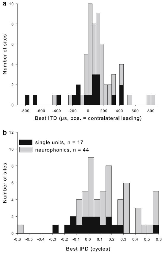
Best ITD and best IPD clustered near zero. Distribution of best ITD (a) and best IPD (b), shown stacked for single units (black bars) and neurophonics (gray bars). The bin width is 50 μs for ITD and 0.05 cycles for IPD

Fig. 6.

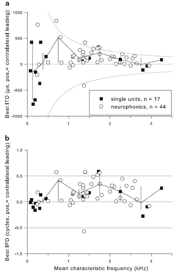
Best ITD showed less scatter with increasing CF. a Best ITD as a function of CF, for all single units (filled squares) and neurophonic recordings (open circles). The black line joins median values in 250 Hz bins below 500 Hz and 500 Hz bins above that, the vertical lines indicate the interquartile range in each bin. Gray lines emphasize zero ITD and ITD-values corresponding to ±0.5 cycles, the so-called π-limit. b Best IPD as a function of CF, shown in the same format as a

3.4 Characteristic phase (CP) and characteristic delay (CD)

CP and CD were determined according to themethods of Yin and Kuwada (1983). All recording sites analyzed conformed to their linearity criteria. Figures 7, 8 and 9 illustrate three examples, a single unit with CF 450 Hz and two neurophonic recordings with CFs at 1.75 and 2.25 kHz, respectively. CPs were expressed on a scale from −0.5 to +0.5 cycles and covered nearly that whole range (−0.49 to +0.45, n = 48). Their distribution was clearly not uniform, with most values (31 of 48 or 68%) falling within ±0.2 (Fig. 10a). The median CP was 0.053. This means that in the majority of cases, the CD fell near a peak in the ITD responses, as for the examples shown in Figs. 7 and 8. Only in a minority of cases did the CD fall closer to a minimum in the ITD responses, as for the example shown in Fig. 9.

Fig. 7.

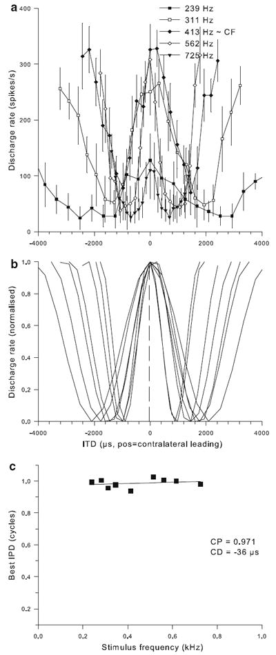
Example of characteristic-delay dataset for a single unit of CF = 450 Hz. a Mean discharge rate (symbols) and standard deviation (vertical thin lines) as a function of ITD for stimulation at five different frequencies around CF, as indicated in the legend. b Cosine fits to the responses at all frequencies tested. Discharge rates are normalized according to the range observed at each frequency. The vertical dashed line indicates the CD value determined as illustrated in c. c Best IPD determined for each of the curves shown in b, as a function of stimulation frequency. The solid line shows the linear regression. Values for characteristic phase and characteristic delay derived from this regression are given in the legend

Fig. 8.

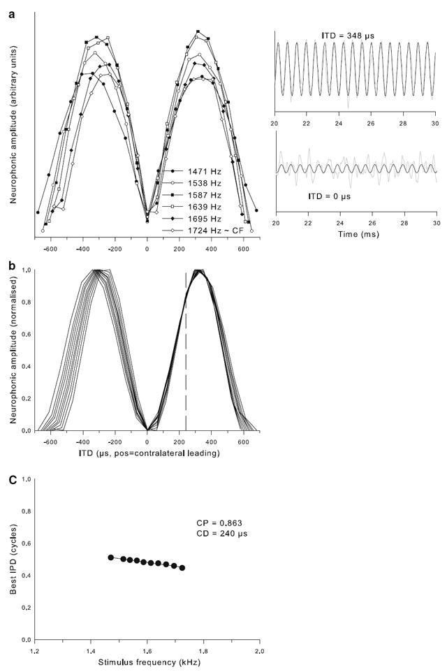
Example of characteristic-delay data set for a neurophonic recording of CF = 1,750 Hz. a Neurophonic response amplitudes as a function of ITD for stimulation at six different frequencies, as indicated in the legend. The two inserts on the right illustrate short segments of the neurophonic waveforms (gray line) averaged over 10 presentations of 1,724 Hz, at the ITDs indicated. Superimposed (black lines) are the cosine fits to the response waveforms. Both panels are scaled identically; note the much-reduced neurophonic amplitude at the unfavourable ITD of 0 μs. b Cosine fits to the response amplitudes over ITD at all frequencies tested. Response amplitudes are normalised according to the range observed at each frequency. The vertical dashed line indicates the CD value determined from the data, as illustrated in c. c Best IPD determined for each of the curves shown in b, as a function of stimulation frequency. The solid line shows the linear regression. Values for characteristic phase and characteristic delay derived from this regression are given in the legend

Fig. 9.

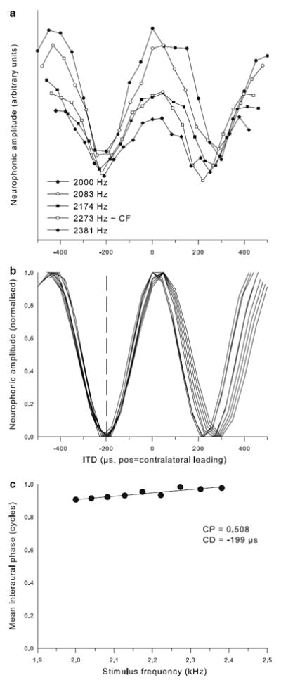
Example of characteristic-delay dataset for a neurophonic recording of CF = 2,250 Hz. The format is the same as for Fig. 8

Fig. 10.

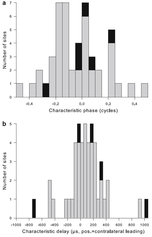
Most recording sites classified as “peakers” and CDs clustered near zero. a Distribution of characteristic phase (CP) values, determined as illustrated in Figs. 7, 8 and 9. Gray bars indicate neurophonic recordings, black bars represent single units. Note that the majority of cases cluster near 0, indicating that ITD selectivities recorded at different frequencies coincided at or near a common peak. b Distribution of CD, shown stacked for single units (black bars) and neurophonics (gray bars). The bin width is 50 μs

CDs ranged from −708 to +1,020 μs with a median of +86 μs (Fig. 10b). Best ITD and CD were significantly correlated (Fig. 11).

Fig. 11.

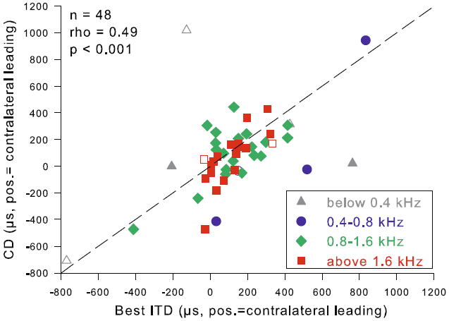
Best ITD and CD were correlated. Best ITD in μs is plotted vs CD. Different frequency ranges are distinguished by different colors, as indicated; open symbols represent single-unit data, closed symbols neurophonic recordings. Statistics for a Spearman rank correlation are given on the top left. The dashed line is a visual reference indicating identical values for both parameters

3.5 Monaural responses predicted best ITD, except at the lowest frequencies

If coincidence detection between inputs from both sides were the main determinant of the binaural sensitivity for ITD, then the monaural responses should predict the best ITD. The difference in delay between ispi- and contralateral click responses was indeed inversely correlated with best ITD for CFs above 0.4 kHz (Fig. 12a, Spearman rank correlation, ρ = −0.68, p < 0.001, n = 35). Similarly, monaural phase responses predicted best ITD very well at CFs above 0.4 kHz (Fig. 12b, Spearman rank correlation, ρ = −0.84, p < 0.001, n = 40). However, these correlations did not hold for CFs below 0.4 kHz where the data scattered a lot more. Here, the difference between monaural click responses did not necessarily agree with the difference between monaural phase responses and neither systematically predicted the best ITD (Fig. 12a, b).

3.6 Best IPD, best ITD and CD were correlated with anatomical position

We successfully labeled 34 recording sites, comprising 4 single units, 28 neurophonic and 2 multi-unit extracellular spike recordings. Two examples are shown in Fig. 13. The chicken NL is tonotopically organized, with the lowest frequencies represented caudolaterally and the highest rostromedially (Rubel and Parks 1975). Accordingly, isofrequency bands run from caudomedial to rostrolateral. Our recording sites covered the full extent of this axis, i.e. labeled sites were found from the medial to the lateral extremes of NL. Best ITD was systematically related to position along the isofrequency axis. This is perhaps most strikingly illustrated by one case where three sites were recorded and labeled along the 1.3 kHz band in an individual NL (Fig. 14). A further seven pairs of recording sites with similar CF from an individual NL where one or both were successfully labeled, and two pairs without label, showed the same trend. Without exception, the best ITD changed towards increasingly contralateral values when moving rostrolaterally within NL. A Wilcoxon test confirmed that this change was highly significant over all pairs (p = 0.001, one-tailed).

Fig. 13.

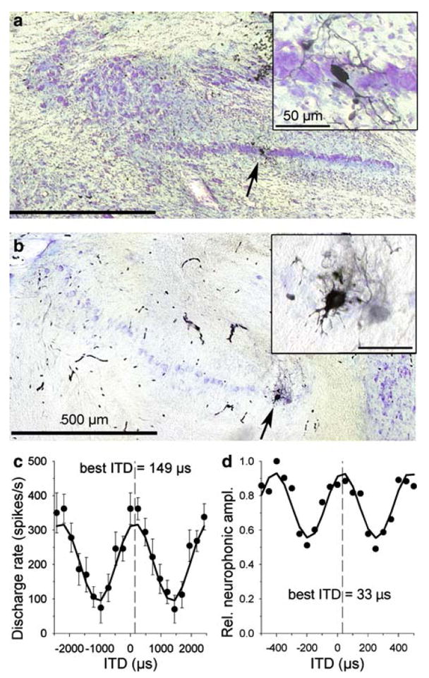
Examples of two labeled recording sites. a, b illustrate the histology. Nissl-stained cross-sections of the brainstem revealed the cellular band of NL (lateral is to the left, dorsal to the top); arrows point to sites with labeled neurons, shown at higher magnification in the inset. c shows the single-unit data corresponding to the label in a; mean discharge rate (± standard deviation) is plotted as a function of interaural time difference, tested at 413 Hz; the solid line is a cosine fit to the data at that same frequency. Best ITD, as determined from the fit, was +149 μs. d shows the neurophonic data corresponding to the label in b; neurophonic amplitude is plotted as a function of interaural time difference, tested at 2,250 Hz; here, the best ITD determined from the cosine fit was +33 μs

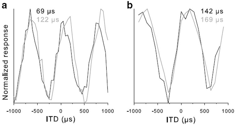
Fig. 14.

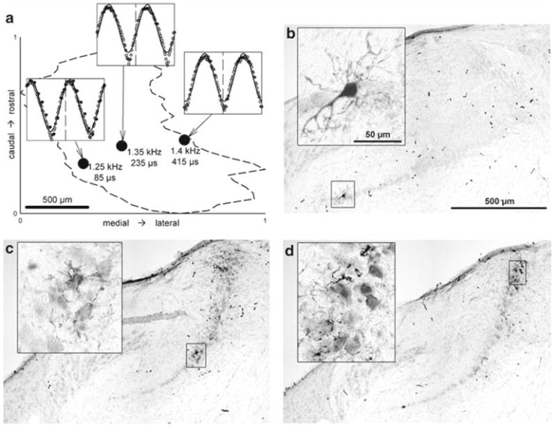
Example of three labeled recording sites from an individual NL illustrating a systematic change of ITD along the isofrequency axis. a Surface view of the NL (dashed outline) as reconstructed from serial cross-sections. The positions of three labeled recording sites are marked and the corresponding CFs and best ITDs indicated next to them. Note the regular change in best ITD with location. The three inserts show the neurophonic amplitudes as a function of ITD recorded at each site and the cosine fits to them; the vertical dashed reference line marks zero ITD in each case. Filled symbols in the left-most panel show the neurophonic measurement repeated after iontophoresis of neurobiotin. b–d illustrate the corresponding histology for those 3 recording sites. The main panel in each case shows an overview of NL (medial is to the left, dorsal to the top). The region of neurobiotin label is box-marked and shown at higher magnification in the insert. At the most medial site (b), a single neuron was filled, while the other two sites (c, d) showed several weakly and less completely labeled neurons as well as some axonal label. Scale bars in b also apply to c and d

In order to normalize and pool the positions of labeled sites across animals we exploited the fact that labeled arbors of NM axons were often seen emanating from the injection site, outlining parts or all of the corresponding isofrequency band. This additional information was used to define the angle of the respective isofrequency band in a reconstructed surface view of the individual nucleus and derive the position of recording sites along these bands (Fig. 15a). In cases without axonal label, the median angle of isofrequency bands (30°), determined from all experiments, was assumed.

Fig. 15.

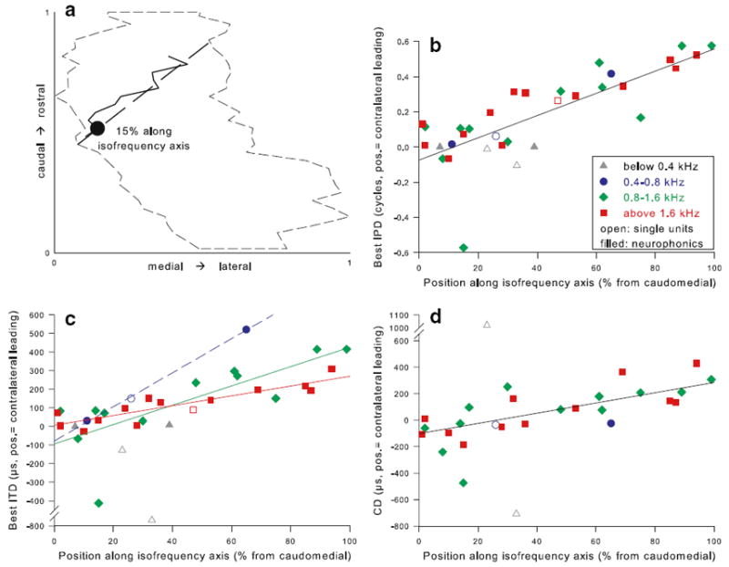
Best ITD, best IPD and CD were represented topographically along the isofrequency axis in NL. a Example of the derivation of normalized position of histologically verified recording sites along the isofrequency axis, for the same case as shown in Fig. 13b, d. The dashed outline is a dorsal view of the individual NL. The filled circle marks the recording site, identified via neurobiotin labeling. The solid line traces the centres of axonal label radiating from the recording site through all sections where label could be found. The dashed line approximates the isofrequency band as a straight line, along which the position of the recording site was determined, in this case at 15% from the caudomedial edge. b Best IPD of all histologically verified recording sites as a function of their position along the respective isofrequency axes. Single-unit recordings are shown as open symbols, neurophonic recordings as closed symbols. Different CF ranges are represented by different symbols and colors as indicated. Best IPD and position along the isofrequency axis correlated significantly (Spearman’s rank correlation test, ρ = 0.77, p < 0.001, n = 33). In addition, a linear regression line is shown (r = 0.78, p < 0.001, n = 33). c The same plot as in b, however the absolute ITD is shown instead of the relative IPD. Best ITD and position along the isofrequency axis also correlated significantly (Spearman’s rank correlation test, ρ = 0.77, p < 0.001, n = 33). Regression lines are shown for the different frequency ranges, in matching colours: blue, 0.4–0.8 kHz (r = 0.99, p = 0.025, n = 3; shown dashed because of marginal significance); green, 0.8–1.6 kHz (r = 0.76, p = 0.004, n = 12); red, above 1.6 kHz (r = 0.89, p < 0.001, n = 14). d CD as a function of position along the isofrequency axis (Spearman’s rank correlation test, ρ = 0.66, p < 0.001, n = 28). A linear regression line for all data is shown (r = 0.72, p < 0.001, n = 26)

There was a highly significant correlation of anatomical position along the isofrequency axis and all three parameters of preferred interaural timing, the best IPD, the best ITD and the CD (Fig. 15b–d). Values close to zero were represented near the caudomedial edge and values corresponding to sounds in the contralateral hemisphere occurred increasingly rostrolaterally. Linear regressions indicated a mapped range for best IPD of 0.63 cycles (−0.07 to +0.56, Fig. 15b) and for CD of 386 μs (−100 to +285, Fig. 15d). Expressed as best ITD (Fig. 15c), the maps furthermore appeared to differ with frequency. Regressions carried out separately for different frequency ranges suggested a mapped range of 518 μs (−94 to +425) for 0.8 to 1.6 kHz, but only 274 μs (+5 to +269) above 1.6 kHz; there were only three data points for the CF-range 0.4–0.8 kHz, which fell along a line covering 915 μs (shown dashed in Fig. 15c). However, these differences in the mapped ITD range remain tentative, as an analysis of covariance for differences in the regression slopes between the frequency ranges did not support them as significant (p = 0.15). A regression over all data of best ITD showed a range of 436 μs (−82 to +354). It remained unclear whether there is a systematic map at all at very low frequencies, below 400 Hz. We have only three labeled sites for this frequency range, all of which were located at similar relative positions along the isofrequency band and scattered widely in their best ITDs.

4 Discussion

The data shown here for the NL of the chicken are among the most comprehensive sets of in vivo recordings from the NL and its mammalian analog, the MSO. Although our sample of single-unit recordings appears small, it is well known that such recordings from the NL and the MSO are difficult to achieve in vivo (e.g. Guinan et al. 1972; Konishi 2003). This is probably due to an unusually small and variable amplitude of spikes in the mature somata of these neurons (Ashida et al. 2007b; Kuba et al. 2006; Scott et al. 2005, 2007). There is thus a crucial difference between recording well-isolated spikes and recording from the cell bodies. In order to achieve simultaneous electrophysiological characterization and histological verification of recording sites within NL, we consistently aimed for the cell body layer, which would have reduced our chances to obtain good single-unit recordings. The majority of recordings reported here are of the neurophonic potential. Intracellular records suggested that the neurophonic potential originates within the NL cells, similar to what has recently been reported for the NL of the barn owl (Ashida et al. 2007a). Furthermore, the neurophonic potential in the chicken is very well localized to the unique cellular monolayer of NL, suggesting its origin in the cells (Schwarz 1992). Finally, neurophonic responses and closely neighboring intracellular or spike responses were very similar. We thus suggest that the neurophonic is a valid reflection of the responses of NL neurons.

Since this is the first extensive characterization of binaural responses from the chicken NL in vivo, we will briefly discuss how the data relate to the well-established concept of coincidence detection. We will then focus on the discussion as to which of the current models of ITD coding is most consistent with the chicken data. This can be broken down into several questions which will be addressed separately: (a) whether there is a systematic representation of ITD, (b) how the neural best ITDs are distributed across the total range found and (c) how the range of neural best ITDs compares to the natural ITD range of the animal. Finally, we will briefly address the implications of our findings for the evolution of ITD coding.

4.1 Coincidence detection and matching of the binaural inputs

NL neurons are excited by monaural stimulation of either ear and, when binaurally stimulated, are sensitive to changes in IPD (e.g., Carr and Konishi 1990). The present data confirmed this for the chicken in vivo. Coincidence detection between the ipsi- and contralateral inputs is thought to underly the sensitivity to IPD in both the avian NL and mammalian MSO (e.g. Grothe et al. 2004). Aprerequisite for coincidence detection is phase-locking to monaural stimulation, which was also confirmed for the chicken NL throughout its CF range.

A crucial test that is commonly employed for in vivo data is that the timing of the monaural responses should predict the ITD of maximal binaural response (Batra and Yin 2004; Carr and Konishi 1990; Goldberg and Brown 1969; Yin and Chan 1990). In the chicken, monaural click and phase responses both predicted best ITD very well, in agreement with coincidence detection. The large scatter observed at the lowest frequencies, below 400 Hz, could be partly due to pronounced interaural canal effects (discussed below) which would have led to deviations of the effective stimuli from what was acoustically presented.

CP should theoretically be zero if coincidence detection between excitatory inputs underlies ITD sensitivity (Yin and Kuwada 1983). Neural values for CP in the MSO indeed always cluster near zero (Batra et al. 1997; Spitzer and Semple 1995; Yin and Chan 1990), as they did in the present study. However, a substantial and as yet unexplained spread is also typical (review in Batra et al. 1997). The variation seen in the chicken was no exception and is thus considered in agreement with coincidence detection.

A final interesting point is that the monaural CFs were, on average, perfectly matched in the chicken, as they are in the NL of the barn owl (Pena et al. 2001). This does not support the stereausis model for NL, which postulates a systematic mismatch in the cochlear locations of origin, and thus CF, between the inputs from both sides as a source of delay (Shamma et al. 1989).

4.2 Maps of ITD and axonal delay lines

The data reported here for the chicken verify a key prediction of the Jeffress model, a topographic representation of a range of best ITD. We found a systematic change of best ITD along the isofrequency axis. This was shown both for individual NL, by multiple recordings within the same isofrequency band, and for recording sites pooled across animals. The representation was restricted to contralateral auditory space, from near zero ITD caudomedially to increasingly contralateral-leading ITDs rostrolaterally. This direction of representation agrees with the anatomical orientation of axonal delay lines in the contralateral inputs (Young and Rubel 1983) and physiological delay lines in vitro (Overholt et al. 1992). Axonal delay lines are the second key element of the Jeffress model.

Very few attempts have been made to date to experimentally test for such maps of ITD at the level of the NL or MSO. The best documented case is the barn owl where a representation of contralateral space was also found (Carr and Konishi 1990; Sullivan and Konishi 1986). There are several interesting differences between the chicken and the owl NL, not least the different anatomical orientation of the ITD maps. However, this is convincingly explained by the hyperplasia of the owl’s NL and its specialisations for high-frequency processing (reviews in Grothe et al. 2004; Kubke et al. 2004). A recent in vitro study on the emu’s NL showed physiological delay lines along the same anatomical axis and in the same direction as in the chicken (MacLeod et al. 2006), supporting the hypothesis that this is the plesiomorphic pattern in birds. We may thus assume that axonal delay lines and maps of ITD, the two key elements of the Jeffress model, are a typical feature of the avian NL. The only mammal where the MSO has been probed for a topographical representation of ITD is the cat. A representation of contralateral space along the rostrocaudal dimension of the nucleus was suggested and is in agreement with the direction of reported axonal delay lines in the inputs. However, the evidence is still tentative and controversial (recent review in Joris and Yin 2007).

Maps of ITD and axonal delay lines are clear evidence in support of the Jeffress model. We believe they also argue against the alternative two-channel model of ITD coding. A central tenet of the latter is a concentration of best IPDs in each frequency band around a uniform value (McAlpine et al. 2001). A certain range of random scatter around the average IPD value might be expected in a biological system; however, a topographic representation of that range is not required, indeed should not exist, if natural selection favored a convergence of best IPD values toward a uniform value. By definition, selection toward a uniform value would select against tuning to different values of IPD and, in consequence, against the formation of a systematic representation of IPD. Parsimony suggests that such maps would not exist without selective pressure to maintain them.

4.3 Distributions of best IPD and best ITD

A distribution in the strictest sense of the Jeffress model should cover the (contralateral) range of natural ITDs, although not necessarily homogeneously (Jeffress et al. 1956). Best IPDs should then show a widening range with increasing CF. In contrast, a distribution in the strictest sense of the two-channel model should be focussed on one particular IPD value across frequencies, typically 45 degrees (McAlpine 2005; McAlpine et al. 2001) and, consequently, will show a regular decrease in best ITD with increasing CF. Real neural distributions usually do not obviously conform to either and their interpretation varies widely, even for comparable sets of data from the same species (Hancock and Delgutte 2004; Yin and Chan 1990). In addition, often the relevant MSO or NL data are not available and inferences have to be made from recordings in their target areas, usually in the midbrain IC. We tend to agree with the recent summary by Joris and Yin (2007) who concluded that, with the exception of the gerbil MSO, all published mammalian MSO and IC data display rather broad distributions which appear incompatible with the narrow predictions of the two-channel model. A constant value of best IPD across frequencies has been suggested (Brand et al. 2002; Hancock and Delgutte 2004; McAlpine et al. 2001), but its significance in the face of substantial scatter remains controversial. For best ITD, what is typically observed is a larger spread of values at lower frequencies (Hancock and Delgutte 2004; Joris et al. 2006; McAlpine et al. 2001) which, of course, corresponds to an increase of average best ITD but is scant evidence for a real relationship between best ITD and frequency.

The chicken NL data reported here were also broadly distributed, but differed in some important aspects. There was no indication for a common best IPD value across frequencies or any discernable trend. Instead, the median best IPD appeared to fluctuate widely (Fig. 6b), consistent with random fluctuations due to minor sampling biases in the different frequency bands. Most interestingly, the scatter was distinctly symmetrical around zero at low frequencies of a few hundred Hz, a fact even more obvious in the distribution of best ITD (Fig. 6a). This is highly unusual and indicates that there is no bias towards a representation of the contralateral auditory hemisphere, as there clearly is at higher frequencies. Although one has to be aware of interaural–canal effects in birds, especially at low frequencies (discussed below), it is difficult to see how that could lead to a sign reversal and thus the erroneous assignment of an ipsilateral-leading best ITD. More likely, the symmetrical scatter around zero reflects an increasing ambiguity in determining the peak of a very broad ITD selectivity curve (Goldberg and Brown 1969) and random CF mismatches, i.e., random differences in the cochlear delays of the inputs from both sides (Joris et al. 2006). In either case, it implies an average value near zero best ITD. This runs contrary to the two-channel model which predicts the best ITDs at such low frequencies to cluster around a large value outside the physiological range (see discussion below). It might be consistent with the Jeffress model, but only if the observed range of best ITDs in this low-frequency range is topographically mapped in NL, which remains open at present. Whether mapped or not, the symmetrical distribution of best ITD around zero indicates a remarkable shift from a predominantly contralateral representation to one of the entire azimuthal space.

The suggestion of a change in ITD representation at low frequencies is intriguing in the light of earlier observations in the barn owl that the low-frequency regions of the NL and its inputs are anatomically different to the higher frequency regions, in a way that suggested a breakdown of the delay-line structure (Köppl and Carr 1997). Unfortunately, physiological data from those low-frequency regions of NL are extremely scarce (Carr and Konishi 1990; Carr and Köppl 2004) and allow no conclusions at present. Wagner et al. (2007). recently published distributions of best ITD for a large sample of owl midbrain neurons. They found an increasing range of best ITD values with decreasing frequency. However, the format that the data were shown in—recordings pooled for both sides of the brain without normalization to ipsi- or contralateral leading—allows no distinction between a symmetrical distribution around zero ITD and a contralaterally biased representation.

In the chicken, the response peak nearest to zero ITD was not always the best ITD, resulting in some best IPDs beyond ±0.5 cycles, outside the so-called π-limit (Fig. 6a). In mammals, neural responses outside the π-limit are rarely observed in the midbrain (Marquardt and McAlpine 2007), in contrast to the barn owl where such responses are a typical feature and well explained by the Jeffress model (Wagner et al. 2007). Interestingly, Marquardt and McAlpine (2007) have suggested that the π -limit may be due to a phase shift underlying interaural delays, as opposed to morphological delay lines. Also, the absence of detectors beyond the π-limit has been attributed to redundancy since the periodicity and relative magnitudes of the peaks in the cross-correlation function beyond the π -limit are not separable (Thompson et al. 2006). The chicken data may be interpreted as both conforming to the π-limit or not, depending on how much significance is attached to the few data points falling outside. Ambiguity in selecting the correct response peak from two similarly sized ones has been blamed for such outliers in mammalian data sets (Marquardt and McAlpine 2007). It is worth pointing out that this can be excluded for the chicken, since the CD and/or monaural responses were used to determine laterality.

In summary, the distribution of best IPD and best ITD in the chicken, as in most other species, are not consistently supportive of either the Jeffress model or the two-channel model. We interpret the substantial scatter of values at any one frequency as more likely compatible with a Jeffress-like code. Intriguingly, the chicken data suggest a shift from the usual contralaterally-biased representation to one centred around zero ITD in the low-frequency regions of NL. This is clearly in conflict with the two-channel model.

4.4 Does the ITD range represented match the chicken’s physiological range?

In order to answer this question, it is important to clarify what the physiological range of ITD in the chicken is. Avian middle ears are not enclosed in bullae as they are in mammals, but are acoustically connected through skull spaces collectively termed the interaural canal. Ears connected like this may function as pressure difference receivers (Calford and Piddington 1988). Depending on the physical dimensions of the head and on the wavelength and the attenuation across the interaural canal, significant interactions between the sounds reaching the eardrum from both sides may result in increased directional cues. Although agreed upon in principle, the precise extent of those effects in different species of birds is still controversial (recent reviews in Klump 2000; Christensen-Dalsgaard 2005). For the chicken, the best measurements of the actual ITD, using cochlear microphonics (Hyson et al. 1994), support a pressure difference receiver mechanism with increasing effect towards lower frequencies. Extrapolating Hyson et al’s. (1994) data to more mature chickens with a head size of up to 25 mm, as used in our experiments, we derive maximal ITDs of about ± 160 μs at high frequencies, rising to ±300 μs at 800 Hz. Below 800 Hz, ITDs for the chicken are unknown, but data from other bird species suggest that they will continue to increase with decreasing frequency (Calford and Piddington 1988; Larsen et al. 1997, 2006). It is important to note that interaural–canal transmission, especially at low frequencies, is severely affected by cumulative changes in skull air pressure under anesthesia (Larsen et al. 1997) and possibly also by tightly sealing sound systems into the ear canals (Rosowski and Saunders 1980), because both the conditions affect eardrum impedance. We assume that middle-ear function was near normal under our experimental conditions, since those conditions were avoided.

An interesting feature of the topographical representation of ITD in the chicken NL was that the mapped range appeared to increase with decreasing frequency—a striking correlation with the physical properties of the middle ear. For the two frequency bands with the most data, 0.8 – 1.6 kHz and >1.6 kHz, the mapped ranges were −94 to +425 μs and −5 to +269 μs. This is a reasonable match with the above estimates of ±300 and ± 160 μs, respectively. Conclusive comparisons must await more extensive measurements of older chickens’ ITD range over a broader frequency range than currently available. Also, the median best ITD of all our recordings in NL fell at +90 μs, clearly within the physiological range of the chicken.

In summary, the ranges of neural best ITD topographically represented in the chicken NL match the estimated physiological ranges well. In addition, the majority of best ITD values clearly fell within physiological range. This is entirely consistent with the Jeffress model of ITD coding. Is it also consistent with the two-channel model? A crucial observation that led to the revival of the two-channel model was that in the guinea pig, many neurons in the IC appear to have their best ITDs outside the animal’s physiological range (McAlpine et al. 2001). According to the predictions in Harper and McAlpine (2004) and using the above estimates for physiological ITDs in the chicken, best ITDs should clearly fall outside the physiological range at low frequencies of a few hundred hertz. The data instead showed a clustering of best ITDs around zero and thus contradict this prediction.

4.5 Implications for the evolution of ITD coding

Taken together, ITD coding in the chicken NL is more broadly consistent with the Jeffress model than with the two-channel model. Thus, contrary to expectations from the optimal coding scheme of Harper and McAlpine (2004), a Jeffress-like place code of ITD could be an evolutionarily stable strategy for an animal with a relatively small head and a limited ability of its neurons to phase-lock to high frequencies. Similarly, Wagner et al. (2007) concluded that ITD coding in the low-frequency range of the barn owl did not conform to the predictions of optimal coding (Harper and McAlpine 2004). This suggests that either ITD coding is not always optimal or that factors not included in the model are of overriding importance. We discuss two such potential factors: no selective pressure for optimal coding and other useful aspects of the neurons’ code.

The relative importance of sound localization in the ecological context of the animal species will impose different selective pressures on the ITD coding circuits (Wagner et al. 2007). Sound localization abilities of the chicken may be optimal for its environment, but not optimal in theoretical terms. This argument, however, simply pushes the problem further back in evolutionary time, as the Jeffress-like layout of the chicken’s ITD coding circuit must have been selected for at some time. Indeed, all available evidence suggests that it is the plesiomorphic condition for birds (Grothe et al. 2004). Paleontological studies show that early birds and their dinosaurian ancestors were predominantly small creatures, similar in head size to pigeons or chickens (review in Chiappe and Dyke 2002), providing no retrospective support for optimal coding.

The usefulness of any neural code for ITD at the level of NL or MSO must depend on how it is read at higher levels of the auditory system. As Takahashi et al. (2003) have pointed out, different aspects of the same neurons’ discharges may be used for different behavioral tasks, e.g. spatial discrimination vs. sound localization, thus rendering the strict distinction between a place code and a population code obsolete. Along similar lines, Joris and Yin (2007) have argued that ITD coding circuits also convey useful information about binaural correlation. Psychophysical studies have shown that humans and owls can localize phantom sound sources well until the correlation declines to a very low value, below which their performance deteriorates (Blauert and Lindemann 1986; Grantham and Wightman 1979; Jeffress et al. 1962; Saberi et al. 1998). Binaural neurons are sensitive to changes in binaural correlation mostly at the peak of the ITD curve and not at the slope (reviewed in Joris and Yin 2007). Thus neurons with best ITDs within the physiological range are most useful for decorrelation detection. These additional constraints suggest that the assumptions of the two-channel model are insufficient. Sensory systems have evolved to extract behaviorally relevant information and organize it into a format that allows subsequent neural stages to process the information rapidly and efficiently (Konishi 1986). The formation of maps of ITD in owls and chickens suggests that such maps engender a profound computational advantage (van Hemmen 2005).

References

- Ashida G, Abe K, Funabiki K. Biophysical mechanism for forming sound-analogue membrane potentials by phase-locked synaptic inputs in owl’s auditory neuron. 30th Midwinter research meeting of the Association for Research in Otolaryngology, Denver. 2007a:148. [Google Scholar]
- Ashida G, Abe K, Funabiki K, Konishi M. Passive soma facilitates submillisecond coincidence detection in the owl’s auditory system. J Neurophysiol. 2007b;97:2267–2282. doi: 10.1152/jn.00399.2006. [DOI] [PubMed] [Google Scholar]
- Batra R, Kuwada S, Fizpatrick DC. Sensitivity to interaural temporal disparities of low- and high-frequency neurons in the superior olivary complex. I Heterogeneity of responses. J Neurophysiol. 1997;78:1222–1236. doi: 10.1152/jn.1997.78.3.1222. [DOI] [PubMed] [Google Scholar]
- Batra R, Yin TCT. Cross correlation by neurons of the medial superior olive: a reexamination. JARO. 2004;5:238–252. doi: 10.1007/s10162-004-4027-4. [DOI] [PMC free article] [PubMed] [Google Scholar]
- Beckius GE, Batra R, Oliver DL. Axons from anteroventral cochlear nucleus that terminate in medial superior olive of cat: observations related to delay lines. J Neurosci. 1999;19:3146–3161. doi: 10.1523/JNEUROSCI.19-08-03146.1999. [DOI] [PMC free article] [PubMed] [Google Scholar]
- Blauert J, Lindemann W. Spatial mapping of intracranial auditory events for various degrees of interaural coherence. J Acoust Soc Am. 1986;79:806–813. doi: 10.1121/1.393471. [DOI] [PubMed] [Google Scholar]
- Brand A, Behrend O, Marquardt T, McAlpine D, Grothe B. Precise inhibition is essential for microsecond interaural time difference coding. Nature. 2002;417:543–547. doi: 10.1038/417543a. [DOI] [PubMed] [Google Scholar]
- Calford MB, Piddington RW. Avian interaural canal enhances interaural delay. J Comp Physiol A. 1988;162:503–510. [Google Scholar]
- Carr CE, Konishi M. A circuit for detection of interaural time differences in the brain stem of the barn owl. J Neurosci. 1990;10:3227–3246. doi: 10.1523/JNEUROSCI.10-10-03227.1990. [DOI] [PMC free article] [PubMed] [Google Scholar]
- Carr CE, Köppl C. Coding interaural time differences at low best frequencies in the barn owl. J Physiol (Paris) 2004;98:99–112. doi: 10.1016/j.jphysparis.2004.03.003. [DOI] [PubMed] [Google Scholar]
- Chiappe LM, Dyke GJ. The mesozoic radiation of birds. Annu Rev Ecol Sys. 2002;33:91–124. [Google Scholar]
- Christensen-Dalsgaard J. Directional hearing in nonmammalian tetrapods. In: Popper AN, Fay RR, editors. Sound source localization. Springer; New York: 2005. pp. 67–123. [Google Scholar]
- Colburn HS, Kulkarni A. Models of sound localization. In: Popper AN, Fay RR, editors. Sound source localization. Springer; New York: 2005. pp. 272–316. [Google Scholar]
- Goldberg JM, Brown PB. Response of binaural neurons of dog superior olivary complex to dichotic tonal stimuli: some physiological mechanisms of sound localization. J Neurophysiol. 1969;32:613–636. doi: 10.1152/jn.1969.32.4.613. [DOI] [PubMed] [Google Scholar]
- Grantham DW, Wightman FL. Detectability of a pulsed tone in the presence of a masker with time varying inter aural correlation. J Acoust Soc Am. 1979;65:1509–1517. doi: 10.1121/1.382915. [DOI] [PubMed] [Google Scholar]
- Grothe B. New roles for synaptic inhibition in sound localization. Nat Rev Neurosci. 2003;4:540–550. doi: 10.1038/nrn1136. [DOI] [PubMed] [Google Scholar]
- Grothe B, Carr CE, Cassedy JH, Fritzsch B, Köppl C. The evolution of central pathways and their neural processing patterns. In: Manley GA, Popper A, Fay RR, editors. Evolution of the vertebrate auditory system. Springer; New York: 2004. pp. 289–359. [Google Scholar]
- Guinan JJ, Norris BE, Guinan SS. Single auditory units in the superior olivary complex. II: locations of unit categories and tonotopic organization. Int J Neurosci. 1972;4:147–166. [Google Scholar]
- Hancock KE, Delgutte B. A physiologically based model of interaural time difference discrimination. J Neurosci. 2004;24:7110–7117. doi: 10.1523/JNEUROSCI.0762-04.2004. [DOI] [PMC free article] [PubMed] [Google Scholar]
- Harper NS, McAlpine D. Optimal neural population coding of an auditory spatial cue. Nature. 2004;430:682–686. doi: 10.1038/nature02768. [DOI] [PubMed] [Google Scholar]
- Hyson RL, Overholt EM, Lippe WR. Cochlear microphonic measurements of interaural time differences in the chick. Hear Res. 1994;81:109–118. doi: 10.1016/0378-5955(94)90158-9. [DOI] [PubMed] [Google Scholar]
- Jeffress LA. A place theory of sound localization. J Comp Physiol Psychol. 1948;41:35–39. doi: 10.1037/h0061495. [DOI] [PubMed] [Google Scholar]
- Jeffress LA, Blodgett HC, Sandel TT, Wood CL. Masking of tonal signals. J Acoust Soc Am. 1956;28:416–426. [Google Scholar]
- Jeffress LA, Blodgett HC, Deatherage BH. Effect of interaural correlation on the precision of centering a noise. J Acoust Soc Am. 1962;34:1122–1123. [Google Scholar]
- Joris PX, Yin TCT. A matter of time: internal delays in binaural processing. Trends Neurosci. 2007;30 doi: 10.1016/j.tins.2006.12.004. [DOI] [PubMed] [Google Scholar]
- Joris PX, Van de Sande B, Louage DH, Van der Heijden M. Binaural and cochlear disparities. Proc Natl Acad Sci USA. 2006;103:12917–12922. doi: 10.1073/pnas.0601396103. [DOI] [PMC free article] [PubMed] [Google Scholar]
- Klump GM. Sound localization in birds. In: Dooling RJ, Fay RR, Popper AN, editors. Comparative hearing: birds and reptiles. Springer; New York: 2000. pp. 249–307. [Google Scholar]
- Konishi M. Centrally synthesized maps of sensory space. Trends Neurosci. 1986;9:163–168. [Google Scholar]
- Konishi M. Coding of auditory space. Ann Rev Neurosci. 2003;26:31–55. doi: 10.1146/annurev.neuro.26.041002.131123. [DOI] [PubMed] [Google Scholar]
- Köppl C. Phase locking to high frequencies in the auditory nerve and cochlear nucleus magnocellularis of the barn owl, Tyto alba. J Neurosci. 1997;17:3312–3321. doi: 10.1523/JNEUROSCI.17-09-03312.1997. [DOI] [PMC free article] [PubMed] [Google Scholar]
- Köppl C, Carr CE. Low-frequency pathway in the barn owl’s auditory brainstem. J Comp Neurol. 1997;378:265–282. [PubMed] [Google Scholar]
- Köppl C, Carr CE. Computational diversity in the cochlear nucleus angularis of the barn owl. J Neurophysiol. 2003;89:2313–2329. doi: 10.1152/jn.00635.2002. [DOI] [PMC free article] [PubMed] [Google Scholar]
- Kuba H, Ishii TM, Ohmori H. Axonal site of spike initiation enhances auditory coincidence detection. Nature. 2006;444:1069–1072. doi: 10.1038/nature05347. [DOI] [PubMed] [Google Scholar]
- Kubke MF, Massoglia DP, Carr CE. Bigger brains or bigger nuclei? Regulating the size of auditory structures in birds. Brain Behav Evol. 2004;63:169–180. doi: 10.1159/000076242. [DOI] [PMC free article] [PubMed] [Google Scholar]
- Larsen ON, Dooling RJ, Ryals BM. Roles of intracranial air pressure in bird audition. In: Lewis ER, Long GR, Lyon RF, Narins PM, Steele CR, Hecht-Poinar E, editors. Diversity in auditory mechanics. World Scientific; Singapore: 1997. pp. 11–17. [Google Scholar]
- Larsen ON, Dooling RJ, Michelsen A. The role of pressure difference reception in the directional hearing of budgerigars (Melopsittacus undulatus) J Comp Physiol A. 2006;192:1063–1072. doi: 10.1007/s00359-006-0138-1. [DOI] [PubMed] [Google Scholar]
- MacLeod KM, Soares D, Carr CE. Interaural timing difference circuits in the auditory brainstem of the emu (Dromaius novaehollandiae) J Comp Neurol. 2006;495:185–201. doi: 10.1002/cne.20862. [DOI] [PMC free article] [PubMed] [Google Scholar]
- Marquardt T, McAlpine D. A pi-limit for coding ITDs: implications for binaural models. In: Kollmeier B, Klump G, Hohmann V, Langemann U, Mauermann M, Uppenkamp S, Verhey J, editors. Hearing—from sensory processing to perception. Springer; Heidelberg: 2007. pp. 407–416. [Google Scholar]
- McAlpine D. Creating a sense of auditory space. J Physiol London. 2005;566:21–28. doi: 10.1113/jphysiol.2005.083113. [DOI] [PMC free article] [PubMed] [Google Scholar]
- McAlpine D, Jiang D, Palmer AR. A neural code for low-frequency sound localization in mammals. NatureNeurosci. 2001;4:396–401. doi: 10.1038/86049. [DOI] [PubMed] [Google Scholar]
- Overholt EM, Rubel EW, Hyson RL. A circuit for coding interaural time differences in the chick brainstem. J Neurosci. 1992;12:1698–1708. doi: 10.1523/JNEUROSCI.12-05-01698.1992. [DOI] [PMC free article] [PubMed] [Google Scholar]
- Palmer AR. Reassessing mechanisms of low-frequency sound localisation. Curr Opin Neurobiol. 2004;14:457–460. doi: 10.1016/j.conb.2004.06.001. [DOI] [PubMed] [Google Scholar]
- Parks TN, Rubel EW. Organization and development of brain stem auditory nuclei of the chicken: Organization of projections from N. magnocellularis to N. laminaris. J Comp Neurol. 1975;164:435–448. doi: 10.1002/cne.901640404. [DOI] [PubMed] [Google Scholar]
- Pena JL, Viete S, Albeck Y, Konishi M. Tolerance to sound intensity of binaural coincidence detection in the nucleus laminaris of the owl. J Neurosci. 1996;16:7046–7054. doi: 10.1523/JNEUROSCI.16-21-07046.1996. [DOI] [PMC free article] [PubMed] [Google Scholar]
- Pena JL, Viete S, Funabiki K, Saberi K, Konishi M. Cochlear and neural delays for coincidence detection in owls. J Neurosci. 2001;21:9455–9459. doi: 10.1523/JNEUROSCI.21-23-09455.2001. [DOI] [PMC free article] [PubMed] [Google Scholar]
- Rosowski JJ, Saunders JC. Sound transmission through the avian interaural pathways. J Comp Physiol. 1980;136:183–190. [Google Scholar]
- Rubel EW, Parks TN. Organization and development of brain stem auditory nuclei of the chicken: Tonotopic organization of N. magnocellularis and N. laminaris. J Comp Neurol. 1975;164:411–433. doi: 10.1002/cne.901640403. [DOI] [PubMed] [Google Scholar]
- Saberi K, Takahashi Y, Konishi M, Albeck Y, Arthur BJ, Farahbok H. Effects of interaural decorrelation on neural and behavioral detection of spatial cues. Neuron. 1998;21:789–798. doi: 10.1016/s0896-6273(00)80595-4. [DOI] [PubMed] [Google Scholar]
- Salvi RJ, Saunders SS, Powers NL, Boettcher FA. Discharge patterns of cochlear ganglion neurons in the chicken. J Comp Physiol A. 1992;170:227–241. doi: 10.1007/BF00196905. [DOI] [PubMed] [Google Scholar]
- Schwarz DWF. Can central neurons reproduce sound waveforms? An analysis of the neurophonic potential in the laminar nucleus of the chicken. J Otolaryngol. 1992;21:30–38. [PubMed] [Google Scholar]
- Scott LL, Mathews PJ, Golding NL. Posthearing developmental refinement of temporal processing in principal neurons of the medial superior olive. J Neurosci. 2005;25:7887–7895. doi: 10.1523/JNEUROSCI.1016-05.2005. [DOI] [PMC free article] [PubMed] [Google Scholar]
- Scott LL, Hage TA, Golding NL. Weak action potential back-propagation is associated with high-frequency axonal firing capability in principal neurons of the gerbil medial superior olive. J Physiol London. 2007;583:647–661. doi: 10.1113/jphysiol.2007.136366. [DOI] [PMC free article] [PubMed] [Google Scholar]
- Shamma SA, Shen N, Gopalaswamy P. Stereausis: binaural processing without neural delays. J Acoust Soc Am. 1989;86:989–1006. doi: 10.1121/1.398734. [DOI] [PubMed] [Google Scholar]
- Smith PH, Joris PX, Yin TCT. Projections of physiologically characterized spherical bushy cell axons from the cochlear nucleus of the cat: evidence for delay lines to the medial superior olive. J Comp Neurol. 1993;331:245–260. doi: 10.1002/cne.903310208. [DOI] [PubMed] [Google Scholar]
- Spitzer MW, Semple MN. Neurons sensitive to interaural phase disparity in gerbil superior olive: Diverse monaural and temporal response properties. J Neurophysiol. 1995;73:1668–1690. doi: 10.1152/jn.1995.73.4.1668. [DOI] [PubMed] [Google Scholar]
- Sullivan WE, Konishi M. Neural map of interaural phase difference in the owl’s brainstem. Proc Natl Acad Sci USA. 1986;83:8400–8404. doi: 10.1073/pnas.83.21.8400. [DOI] [PMC free article] [PubMed] [Google Scholar]
- Takahashi TT, Bala ADS, Spitzer MW, Euston DR, Spezio ML, Keller CH. The synthesis and use of the owl’s auditory space map. Biol Cybern. 2003;89:378–387. doi: 10.1007/s00422-003-0443-5. [DOI] [PubMed] [Google Scholar]
- Thompson SK, von Kriegstein K, Deane-Pratt A, Marquardt T, Deichmann R, Griffiths TD, McAlpine D. Representation of interaural time delay in the human auditory midbrain. Nature Neurosci. 2006;9:1096–1098. doi: 10.1038/nn1755. [DOI] [PubMed] [Google Scholar]
- van Hemmen JL. What is a neuronal map, how does it arise, and what is it good for? In: Van Hemmen JL, Sejnowski TJ, editors. 23 problems in systems neuroscience. Oxford University Press; Oxford: 2005. pp. 83–102. [Google Scholar]
- Viete S, Pena JL, Konishi M. Effects of interaural intensity difference on the processing of interaural time difference in the owl’s nucleus laminaris. J Neurosci. 1997;17:1815–1824. doi: 10.1523/JNEUROSCI.17-05-01815.1997. [DOI] [PMC free article] [PubMed] [Google Scholar]
- Wagner H, Brill S, Kempter R, Carr CE. Microsecond precision of phase delay in the auditory system of the barn owl. J Neurophysiol. 2005;94:1655–1658. doi: 10.1152/jn.01226.2004. [DOI] [PMC free article] [PubMed] [Google Scholar]
- Wagner H, Asadollahi a, Bremen P, Endler F, Vonderschen K, Von Campenhausen M. Distribution of interaural time difference in the barn owl’s inferior colliculus in the low- and high-frequency ranges. J Neurosci. 2007;27:4191–4200. doi: 10.1523/JNEUROSCI.5250-06.2007. [DOI] [PMC free article] [PubMed] [Google Scholar]
- Yin TCT. Neural mechanisms of encoding binaural localization cues in the auditory brainstem. In: Oertel D, Fay RR, Popper AN, editors. Integrative functions in the mammalian auditory pathway. Springer; New York: 2002. pp. 99–159. [Google Scholar]
- Yin TCT, Chan JCK. Interaural time sensitivity in the medial superior olive of the cat. J Neurophysiol. 1990;64:465–488. doi: 10.1152/jn.1990.64.2.465. [DOI] [PubMed] [Google Scholar]
- Yin TCT, Kuwada S. Binaural interaction in low-frequency neurons in inferior colliculus of the cat. III. Effects of changing frequency. J Neurophysiol. 1983;50:1020–1042. doi: 10.1152/jn.1983.50.4.1020. [DOI] [PubMed] [Google Scholar]
- Young SR, Rubel EW. Frequency-specific projections of individual neurons in chick brainstem auditory nuclei. J Neurosci. 1983;3:1373–1378. doi: 10.1523/JNEUROSCI.03-07-01373.1983. [DOI] [PMC free article] [PubMed] [Google Scholar]
- Yin TCT, Chan JCK, Carney LH. Effects of interaural time delays of noise stimuli on low-frequency cells in the cat’s inferior colliculus III. Evidence for cross-correlation. J Neurophysiol. 1987;58:562–583. doi: 10.1152/jn.1987.58.3.562. [DOI] [PubMed] [Google Scholar]