Swimming direction reversal of flagella through ciliary motion of mastigonemes

Abstract

Bio-inspired designs can provide an answer to engineering problems such as swimming strategies at the micron or nano-scale. Scientists are now designing artificial micro-swimmers that can mimic flagella-powered swimming of micro-organisms. In an application such as lab-on-a-chip in which micro-object manipulation in small flow geometries could be achieved by micro-swimmers, control of the swimming direction becomes an important aspect for retrieval and control of the micro-swimmer. A bio-inspired approach for swimming direction reversal (a flagellum bearing mastigonemes) can be used to design such a system and is being explored in the present work. We analyze the system using a computational framework in which the equations of solid mechanics and fluid dynamics are solved simultaneously. The fluid dynamics of Stokes flow is represented by a 2D Stokeslets approach while the solid mechanics behavior is realized using Euler-Bernoulli beam elements. The working principle of a flagellum bearing mastigonemes can be broken up into two parts: (1) the contribution of the base flagellum and (2) the contribution of mastigonemes, which act like cilia. These contributions are counteractive, and the net motion (velocity and direction) is a superposition of the two. In the present work, we also perform a dimensional analysis to understand the underlying physics associated with the system parameters such as the height of the mastigonemes, the number of mastigonemes, the flagellar wave length and amplitude, the flagellum length, and mastigonemes rigidity. Our results provide fundamental physical insight on the swimming of a flagellum with mastigonemes, and it provides guidelines for the design of artificial flagellar systems.

INTRODUCTION

The concept of micro-fluidic devices such as lab-on-a-chip is finding many applications in bio-medical science, especially in bio-chemical diagnosis. The main advantage of such micron-scale devices is that they require a very small volume of liquid to perform a complicated and complete diagnosis of biological samples. A typical lab-on-a-chip device has many micro-labs connected through micro-channels, and the biological samples are transported for detailed bio-chemical analysis via externally generated fluid flow in the channels. However, the flexibility to create diverse flow patterns in these devices is limited, which makes micro-object transport at these length scales difficult to control.

Artificial micro-swimmers could be used for micro-object manipulation in lab-on-a-chip devices and in targeted drug delivery applications. The primary challenge in the design of such a micro-swimmer is that the swimming strategies at these length scales are difficult to achieve using external triggers.^{1, 2, 3, 4, 5, 6} Bio-inspired design can provide an answer to such engineering problems. Many micro-organisms swim by the use of hair-like projections known as flagella. Spermatozoa use an undulating flagellum for propulsion (see Fig. 1a) while Paramecia rely on the asymmetric motion of cilia. Cilia and flagella are biological systems with a similar micro-structure and working principle. The undulations in the cilium or flagellum are driven by motor proteins which causes propulsion of the micro-organism in the fluid. Cilia and flagella play an important role in micro-organism swimming and are widely explored in the literature.^{1, 2, 7} Where the working principle of flagella is exploited to design artificial micro-swimmers,^{5, 8, 9, 10} the cilium principle is used to design fluid flow and mixing devices at the micron and nano-scale.^{11, 12, 13}

Figure 1.

(a) Flagellar oscillation of a ram spermatozoon. The cell is moving forward by altering the bend curvature and thus propagating the wave. The scale bar is 10 μm.²⁰ (b) Ochrophyte with a flagellum bearing mastigonemes.²¹ (Figures are reproduced with permission of the copyright owner(s).)

Micro-organisms exist that have flagella with vertical appendages over their length,^{7, 14, 15} see Fig. 1b. These appendages are known as mastigonemes and can cause a swimming direction reversal relative to the wave propagation along the length of the flagellum.^{7, 14, 15, 16} Where a smooth flagellum swims in a direction opposite to the traveling wave, a flagellum bearing mastigonemes would swim in the direction of the traveling wave.^{7, 14, 15, 16, 17, 18, 19} Although the working principle of micro-organisms swimming by flagellar or ciliary motion is widely explored, the class of flagellar micro-organisms bearing mastigonemes has not been intensively studied. In a micro-fluidic application such as lab-on-a-chip in which micro-object manipulation in small flow geometries is required, control of the swimming direction becomes an important aspect. Understanding how nature controls the swimming direction at typical micro-fluidic length and timescales can provide guidelines for bio-inspired design of artificial micro-swimmers. This is explored in the current paper for flagellated systems that are covered with mastigonemes. We analyze the relation between the swimming direction and the mastigoneme structure and aim at understanding the physical origin of thrust reversal.

In the past, efforts have been made to analyze thrust reversal associated to the presence of the mastigonemes on a smooth flagellum.^{14, 15, 16, 17, 18, 19} To explain the thrust reversal, it has been qualitatively proposed (based on laboratory observations and curve fitting) that the presence of the mastigonemes decreases the ratio of normal to tangential drag coefficients (C_n/C_t) from a value of 2 (affirmed for a smooth flagellum) to 0.5.¹⁴ Later a more detailed hydrodynamic analysis of a flagellum bearing mastigonemes was presented by Brennen,¹⁶ using an analytical approach (resistive force theory) based on the assumption of hydrodynamically non-interacting mastigonemes and assuming small-amplitude deflections. This limits the applicability of such analytical solution in situations where the mastigonemes are taller and/or tightly packed and in case of large-amplitude flagellar waves. Evidence (experimental and computational) exists that the mastigonemes can reverse the direction of swimming,^{14, 15, 17, 18} but the conditions at which this is possible are not explicitly quoted in the literature. To overcome these limitations, we propose a solid-fluid interaction model that fully accounts for hydrodynamic interactions and large amplitude undulations as well as non-linear mastigoneme deformations. We investigate the swimming problem of a flagellum bearing mastigonemes with an aim to explore the fundamental mechanism responsible for swimming direction reversal and study the swimming velocity as a function of the system parameters.

COMPUTATIONAL MODEL AND APPROACH

Swimming of a micro-organism is a fluid-solid interaction (FSI) problem, where the continuum equations for the micro-organism motion/deformation have to be simultaneously solved with the fluid dynamics equations. The Stokeslet approach can be used in the present context since the swimming dynamics of the micro-organisms is governed by the Stokes flow equations in which inertial forces are negligible.^{22, 23, 24} In the present work, an integral formulation for 2D-Stokes flow is implemented using the boundary element method to represent the fluid environment while the micro-organism itself is represented by a collection of 2D beam elements. Coupling of the solid mechanics and the fluid dynamics equations are done in an implicit manner as suggested by Khaderi and Onck,²⁵ and details of the computational approach are given in the . Our analysis is similar to the analysis performed by Taylor,¹ in which the swimming of an infinite sheet has been analyzed. The obtained swimming velocity was shown to have a similar (qualitative) dependence on the amplitude, wavelength and frequency of the wave; compared to the flagellar swimming velocity obtained by using resistive force theory and slender-body-theory that are 3D in nature.^{2, 22, 26, 27}

To understand and explore the key principle behind the thrust force/direction reversal with the presence of mastigonemes over the flagellum length, we prescribe flagellar beating with the wave propagating in the positive x-direction (i.e., to the right in Fig. 2), according to

$$y(x,t)=A\sin (\omega t-\mathit{kx}),$$ (1)

where x and t are the position and time, respectively, ω = 2π/t_cycle and k = 2π/λ. The micro-swimmer (flagellum and mastigonemes) and the characteristic length scales are depicted in Fig. 2. The elastic properties of the micro-swimmer are defined by Young’s modulus (E) and Poisson’s ratio (ν). The viscous drag forces of the fluid are considered via a 2D Stokeslet approach and are proportional to the viscosity (μ) of the fluid. During the simulations, we prescribe the transverse velocity (V_kp) for the base flagellum only. The equations of motion are then solved using the finite element method where the drag forces (T_d) are evaluated on-the-fly using the Stokeslets approach (T_d =G⁻¹V_kp), where the Green’s function (G) relates the micro-swimmer velocity to the traction forces of the fluid. As an outcome of the traction forces acting on the micro-swimmer’s surface/boundary, the micro-swimmer swims in the forward or backward direction with a net propulsive velocity, U. Finally, we determine the velocity distribution in the fluid domain, U_fluid due to the swimming motion of the micro-swimmer using U_fluid = G₁T_d, where G₁ relates the velocities in the fluid to the drag forces on the micro-swimmer.

Figure 2.

Illustration of a flagellum bearing mastigonemes. L is the length of the flagellum, A and λ are the amplitude and wave length of wave deformation, H and ΔS are the height and spacing between the mastigonemes, respectively, and h is the thickness of the mastigonemes.

DIMENSIONAL ANALYSIS AND SIMULATION RESULTS

A dimensional analysis has been performed to explore the influence of the parameters involved in the system and specifically under which conditions the mastigonemes reverse the swimming direction. A flagellum bearing mastigonemes consists of five important length parameters as illustrated in Fig. 2, which are (1) the amplitude of the wave deformation (A), (2) the wave length (λ), (3) the length of the base flagellum (L), (4) the height of the mastigonemes (H), and (5) the spacing between the mastigonemes (ΔS). The rigidity of the mastigonemes is defined by the bending modulus (EI), where E is Young’s modulus and I is the moment of inertia. By performing a dimensional study to explore the influence of each variable on the system dynamics, we obtain four dimensionless length parameters, A* = A/λ, H* = H/λ, L* = L/λ, 1/N_m =ΔS/λ, and one force parameter F_m = 12μkAωH³/Eh³, which defines the ratio of viscous forces over the elastic forces.¹¹ Note that the parameter F_m can be seen as the ratio of two time scales: an imposed time scale by the periodic oscillations of the flagella (dθ∕dt∝kAω) and a response time scale of the mastigonemes related to the frictional properties (μH³/Eh³). The strong dependence of F_m on h (power 3) stems from the moment of inertia (I∝h³) and leads to a profound increase of F_m for floppy mastigonemes. For the present study, we keep ω and λ constant and change other parameters to alter the dimensionless variables.

Assuming that the mastigonemes are rigid (by selecting the values for the parameters such that F_m = 0.001 with λ = 100 μm and t_cycle = 10 ms) and L* = 1, the influence of all other dimensionless parameters is shown in Fig. 3. For a given value of A* and H* the net propulsive velocity (U) is being plotted for various values of N_m, with N_m = λ/ΔS the number of mastigonemes per wavelength of the base flagellum. For a smooth flagellum (N_m = 0) the swimming velocity is negative, i.e., the flagellum swims to the left. For all the heights of the mastigonemes (H*), a saturation in the swimming velocity (U) is observed with an increase in the number of mastigonemes per wave length (N_m). The presence of mastigonemes reduces the swimming velocity, and a further increase in the height of the mastigonemes can even cause a reversal in the swimming velocity (i.e., positive U in Fig. 3).

Figure 3.

Influence of the dimensionless variables A*, H* and N_m on the net propulsive velocity for L* = 1 and F_m = 0.001. The presence of the mastigonemes reduces the swimming velocity, and a further increase in height H can even cause reversal of the swimming direction.

To analyze the system further, we choose N_m to be 16 (where a saturation in the swimming velocity is observed, see Fig. 3). Trends in the swimming velocity (U) with respect to A* are shown in Fig. 4a for various values of H* and for L* = 1. As can be seen from Fig. 4a, the swimming velocity (U) appears to have a quadratic dependence on A* for all values of H*. One can normalize the swimming velocity (U) with the swimming velocity of the smooth flagellum (U^f) for a given A*. This normalized swimming velocity (U* = U/U^f) is linear in H* and independent of A* as shown in the inset of Fig. 4a. The role of L* on the swimming velocity is shown in Fig. 4b for various H* and for A* = 0.05, N_m = 16. The swimming velocity saturates at higher L* values, and the role of L* can be seen as a finite size effect (or end effect) that disappears for higher values of L*. It can be noted that for the smooth flagellum the swimming velocity converges to the swimming velocity of an infinite sheet as suggested by Taylor.¹ The effect of L* on the normalized velocity U* is small however, see the inset of Fig. 4a. This suggests that for the rigid mastigonemes the swimming direction reversal is only dictated by H* and is independent of A* and L* (for L* > 2), see inset of Fig. 4a. To verify this, a simple first-order calculation can be performed based on the resistive force theory suggested by Gray and Hancock.² Given the motion of the base flagellum Y_f = A sin(ωt – kX_f), the motion of the mastigoneme can be written as X_m = X_f – ssin(θ) and Y_m = Y_f + scos(θ), where, ω = 2π/t_cycle, k = 2π/λ, θ = arctan(dY_f/dX), and s varies from –H to H. By assuming that $C_t^f$ and $C_n^f$ are the flagellum’s drag coefficients in the tangential and normal direction, respectively, we can write the x-component of total force on the smooth flagellum as

$$F_x^f=\frac{2A^2{\pi }^2(C_n^f-C_t^f)+C_t^f\lambda t_{\mathit{cycle}}U}{t_{\mathit{cycle}}}.$$ (2)

Similarly, by assuming that $C_t^m$ and $C_n^m$ are the mastigoneme’s drag coefficients, we can write the total force on one mastigoneme as

$$F_x^m=2H\left\{\frac{2A^2{\pi }^2(C_t^m-C_n^m)+C_n^m\lambda t_{\mathit{cycle}}U}{\lambda t_{\mathit{cycle}}}\right\}.$$ (3)

For both flagellum and mastigonemes the total force consists of a propulsive part due to actuation forces (the first part in Eqs. 2, 3) and a retarding part due to the drag forces opposing the horizontal swimming velocity (the second part in Eqs. 2, 3). When the flagellum with N_m mastigonemes reaches a steady state swimming velocity U, the propulsive and retarding forces are in (dynamic) equilibrium, so that the total force must be zero.

$$F_x^f+N_m{F}_x^m=0,$$ (4)

which leads to

$$U=\frac{-2{\pi }^2{A}^2}{\lambda t_{\mathit{cycle}}}\left\{\frac{\lambda (C_n^f-C_t^f)-2{\mathit{HN}}_m(C_n^m-C_t^m)}{\lambda C_t^f+2{\mathit{HN}}_m{C}_n^m}\right\},$$ (5)

and can be written in the form

$$U^{*}=U∕U^f=\frac{(C_n^f∕C_t^f-1)-2({\mathit{HN}}_m∕\lambda )\{(C_n^m-C_t^m)∕C_t^f\}}{1+2({\mathit{HN}}_m∕\lambda )(C_n^m∕C_t^f)}.$$ (6)

The form of this expression is very similar to what is suggested by Brennen.¹⁶ Our simulation results show a similar quadratic dependence on A (see Fig. 4a) and a linear dependence on frequency (results not shown). Also, the above equation indicates that the normalized velocity (U*) is independent of A* as shown in the inset of Fig. 4a. It can be clearly seen from the above expression that for $C_n^f∕C_t^f>1$ and $C_n^m∕C_t^m>1$, the very presence of the mastigonemes will reduce the resultant velocity and can possibly reverse the direction of swimming. In Eq. 6 direction reversal can be achieved by either increasing H/λ or N_m, in accordance with our simulations (see Fig. 3). However, the collapse of these effects into one single parameter, HN_m/λ, is not in accordance with our simulations and is a consequence of the assumptions made in Eq. 6. Apart from the assumption of small deformations, the critical assumption for deriving this expression was to ignore any hydrodynamic interaction (either between the mastigonemes or with the base flagellum) present in the system. This implies that the above expression should be interpreted with care. Most importantly, it emphasizes the need for a fully coupled hydrodynamic analysis to understand the associated physics.

Figure 4.

(a) Swimming velocity as a function of A* for various values of H* and for L* = 1, N_m = 16. Inset: normalized swimming velocity (U* = U/U^f) as a function of H*, where U^f is the swimming velocity of the smooth flagellum for a given A*. The normalized swimming velocity is independent of A* and L* (for L* > 2). (b) The role of L* (finite size effect) on the swimming velocity for various values of H* and for A* = 0.05, N_m = 16.

Next, we further explore the hydrodynamic origin of swimming direction reversal by looking at the system from a fluid propulsion point-of-view. Here, we analyze a horizontally-static flagellum with (and without) mastigonemes by fixing the x-position of the left end of the flagellum but still allowing the transverse displacements and rotations caused by the traveling wave. The pressure field with the streamlines are shown in Fig. 5 for the smooth flagellum and for the flagellum bearing mastigonemes. As the base flagellum is propagating a wave (in the positive x-direction), the surrounding fluid acquires vortices of alternating sign along the length of the micro-swimmer. The vorticity is positive (i.e., counter clockwise) near the flagellum crests and is negative (clockwise) near the flagellum valleys. The effective flow velocity (shown by the curved red arrows) indicates the direction of the fluid propulsion which changes sign in the presence of the mastigonemes, compare Fig. 5a to Fig. 5c. In the case of a smooth flagellum the effective flow velocity is to the right (in the direction of the traveling wave), which causes the smooth flagellum to swim (if released) in the negative x-direction (opposite to the direction of the traveling wave),⁶ see Fig. 4b. However, for the flagellum bearing mastigonemes the effective flow velocity is to the left (see Fig. 5c) and will cause swimming in the positive x-direction (in the direction of the traveling wave). Note that in the case of mastigonemes of height H* = 1/8, the regimes of high pressure and low pressure are opposite to the smooth flagellum, confirming the reversal of swimming direction. Interestingly, for the flagellum bearing mastigonemes of height H* = 1/16 there is no apparent direction of the fluid flow (only vortices), which indicates that the swimming velocity is approximately zero as can be seen from Fig. 4.

Figure 5.

Pressure field with streamlines for the smooth flagellum (a) and for the flagellum bearing mastigonemes (b) and (c), for A* = 0.1 and L* = 3. The contours represent the pressure value (blue and red colors represent a pressure of −0.5 N/m² and +0.5 N/m², respectively). The micro-swimmer is represented by the thick white line, and the base flagellum is constrained not to swim, however still propagating a wave in the positive x-direction (by fixing the x-position of the left end of the flagellum but allowing the transverse displacement and rotation). The effective flow velocity (shown by the curved red arrows) indicates the direction of the fluid flow, which changes sign in the presence of the mastigonemes. Note that in the presence of mastigonemes of height H* = 1/8 (c), the regimes of high pressure and low pressure are opposite to the smooth flagellum case (a).

Next we will explore the effect of deformable mastigonemes on the swimming direction reversal. As the dimensionless variable F_m defines the ratio of viscous forces over the elastic forces, it can be used to quantify the flexibility of the mastigonemes. In Fig. 6a the normalized swimming velocity (U*) is plotted against H* for various values of F_m. The influence of the mastigoneme flexibility (F_m) on the swimming velocity is shown in the inset for H* = 0.125. As shown in Fig. 6, the rigid mastigonemes (F_m < 0.1) are more effective in reducing the swimming velocity or swimming direction reversal,¹⁶ and floppy mastigonemes F_m > 2 can not reverse the swimming direction due to the mastigonemes deformation, see Fig. 6b. At higher F_m values the flexible mastigonemes deform due to the fluid forces and are not able to effectively respond to the imposed basal angular oscillations, so that the mastigonemes attain a deformed configuration (see Fig. 6b). As a result, the floppy mastigonemes do not displace the surrounding fluid as effective as the rigid ones (this will be discussed later with reference to Ref. 28), so that the floppy mastigonemes cannot counteract the flow caused by the base flagellum as effectively as their rigid counter-parts. An animation of the resulting motion by flexible and rigid mastigonemes subjected to the same basal oscillation is included as supporting information (see Ref. 28).

Figure 6.

(a) The normalized swimming velocity as a function of H* for various values of F_m and N_m = 8, A* = 0.1, and L* = 1. Mastigonemes can be treated as rigid when F_m ≤ 0.1. The influence of the mastigoneme flexibility (F_m) on the swimming velocity is shown in the inset for H* = 0.125. (b) Swimming of the flagellum bearing mastigonemes where the arrow represents the swimming direction. Flexible mastigonemes deform due to the viscous forces and are ineffective (compared to the rigid mastigonemes) in causing direction reversal.

Interestingly, flattening of the curves can be observed for taller mastigonemes (and larger F_m values) and is due to the fact that the deformed mastigonemes start interacting with each other (or with the base flagellum). As a result, with increasing F_m and H the deformed shape of the mastigonemes converges to a specific shape since hydrodynamic (lubrication) interactions prevent them from coming any closer to each other and to the base flagellum. It should also be noted that the deformed shape of the flexible mastigonemes in Fig. 6b is a direct consequence of the external flow created by the base flagellum. Subjecting an isolated mastigoneme (i.e., in the absence of the base flagellum) to similar periodic oscillations of the base displacement and basal angle results in negligible deformation of the mastigoneme. Clearly, the flow generated by the base flagellum plays a key role in deforming the flexible mastigonemes, and it is because of this flow that the floppy mastigonemes generate an opposing flow.

MASTIGONEMES WORK AS METACHRONIC CILIA

It has been suggested that the mastigonemes project rigidly from the flagellar surface and interact with the surrounding fluid while acting like paddles that are swept laterally as the wave propagates along the flagellum.¹⁵ In the following we will explore the relation between the paddling motion of the mastigonemes and the direction reversal mechanism and try to quantify the observed trends. We will address these issues by linking the mastigoneme motion to the working principle of cilia. Later, we will use the envelope theory⁷ to obtain the net propulsive velocity generated by the envelope formed with the mastigonemes tips on an undulating flagellum.

We consider a non-propelling flagellum in a fluid by fixing the position of the left end of the flagellum (but allowing it to rotate and move in the transverse direction). As a result, the wave propagation during the flagellar beat cycle will push the fluid rather than causing swimming of the flagellum. Fluid propulsion at various time instances of the flagellar beat is shown in Fig. 7, where the base flagellum is propagating a wave in the positive x-direction. The thick white line represents the micro-swimmer, and the broken white line indicates the initial position of the fluid particles. The simulations show that for a smooth flagellum, the fluid particles are being displaced in the direction of wave propagation while the particles are being displaced in the opposite direction in the presence of mastigonemes (see Fig. 7). The contours represent the horizontal velocity of the fluid (blue and red colors represent a velocity of −1.5 mm/s and +1.5 mm/s, respectively). Note that for the smooth flagellum the average fluid velocity is positive (red color) at all time instances, which causes the fluid propulsion to the right (in the direction of the traveling wave). However, in the presence of mastigonemes of height H* = 1/8, the average fluid velocity is negative (blue color) at all time instances causing the fluid propulsion to the left (in the direction opposite to the traveling wave).

Figure 7.

Fluid propulsion at various time instances (indicated in the middle column) of the flagellum beat. The thick white line represents the micro-swimmer. The broken white line indicates the initial position of the fluid particles. The contours represent the horizontal velocity of the fluid (blue and red colors represent a velocity of −1.5 mm/s and +1.5 mm/s, respectively). The arrow represents the velocity vector of the tracked particle. Left: smooth flagellum. Right: flagellum bearing mastigonemes of height H* = 1/8. The area swept by the mastigonemes is shown with the solid back line, where the curved arrows represent the direction of motion. The base flagellum is propagating a wave in the positive x-direction.

These results are in correspondence with the results reported in the literature.^{14, 15, 16, 17, 18} When a wave propagates along a smooth flagellum the region of the flagellum between the wave crests and valleys exerts substantial forces on the fluid in the wave propagation direction. The wave crests and valleys, however, do not contribute to propulsion but predominantly experience tangential drag forces due to the steady state swimming velocity of the flagellum (or due to the external fluid flow in case of a non-propelling flagellum).¹⁹ We have seen that for the smooth flagellum the resultant flow will be in the direction of wave propagation, and this scenario changes with the presence of external appendages (mastigonemes) over the flagellum length. These mastigonemes project rigidly from the flagellar surface and interact with the surrounding fluid while acting like paddles that are swept laterally as the wave propagates along the flagellum. The base flagellum pushes the fluid in the direction of wave propagation while the mastigonemes push the fluid in the opposite direction (see Figs. 57). In fact, each individual mastigoneme acts as a cilium (effective stroke in the opposite direction of wave travel) and sweeps an area causing propulsion in the direction opposite to the wave propagation as shown in Fig. 7 (see the right image). The area swept by the tip of the mastigoneme is shown with the solid back line where the curved arrow represents the direction of motion. Interestingly, due to the beating of the base flagellum, the upper and lower mastigonemes are synchronized in such a fashion that when the upper mastigoneme is in effective stroke, the lower mastigoneme executes the recovery stroke. Thus, the mastigonemes work like co-operating cilia whose motion is driven by the motion of the base flagellum. Due to the wavelike motion of the base flagellum the collective motion of the mastigonemes resembles the metachronic motion of cilia. Since the effective stroke of the mastigonemes is in a direction opposite to the traveling wave of the base flagellum, the mastigonemes feature an antiplectic metachrony.²⁹

Fluid dynamics in the Stokes-regime is dominated by viscosity rather than inertia. An important consequence is that fluid propulsion can only be achieved when the motion is spatially asymmetric. This is achieved in nature by cilia going through a series of different shapes as illustrated in Fig. 8a, consisting of an effective and a recovery stroke. During the effective stroke the cilium stands high and pushes the fluid, while during the recovery stroke, it remains low to limit the back flow, which results into fluid flow in the direction of the effective stroke. Natural cilia use an internal forcing system based on motor proteins to achieve the shape changes. However, the asymmetric motion achieved by the mastigonemes is only due to the basal oscillation and is shown in Fig. 7. The stiffer the mastigoneme, the larger the asymmetric motion (see Fig. 8b), resulting in a larger swept area and thus a larger fluid flow.^{11, 30} Clearly, a larger deformation in case of internally driven cilia increases flow, while a larger deformation in case of base-driven mastigonemes reduces flow.

Figure 8.

Working principle of the mastigonemes (cilium). (a) Cilium beat cycle and the area swept during the effective and the recovery strokes. The resultant fluid flow is in the direction of the effective stroke. (b) Trajectory of the tip of the mastigoneme and its dependence on H* (left) and A* (middle). The tip’s trajectory resembles an ellipse, where A and Hsin{arctan (2πA/λ)} are the major and minor axis of the ellipse shown by the vertical and horizontal arrows, respectively. At higher F_m values the area swept reduces due to the deformation of the mastigonemes (see Fig. 6b). An animation of the swept-area by flexible and rigid mastigonemes is included as supplementary material (Ref. ²⁸).

In the numerical study performed by Khaderi and coworkers,^{11, 30} it was shown that during (planar) asymmetric beating of a cilium, a non-zero area is swept by the cilia tip that can be used to quantify the net fluid displaced (a linear relation was found between the swept area and fluid flow). For example, if a cilium traces the same path during the effective and recovery stroke, the area swept by the tip will be zero, resulting in a similar amount of fluid displaced during the effective and recovery stroke. When the cilium follows a path that is different during the recovery stroke, symmetry is broken, leading to a non-zero swept area and a net fluid flow due to the difference in forward and backward flow. The dependence of the area swept by the mastigonemes on the amplitude of the flagellar motion (A) and the height of the mastigonemes (H) is shown in Fig. 8b. The tip’s trajectory of the mastigoneme resembles an ellipse, whose area is πAHsin{arctan(2πA/λ)}. For small values of A/λ, this reduces to the simple expression 2π²HA²/λ, clearly explaining the linear dependence on H and the quadratic dependence on A of the net propulsive velocity (see Fig. 4a). The number of the mastigonemes per wave length of the base flagellum (N_m) can be seen as the density of the cilia (ΔS being the inter-cilia spacing), and it has been shown that the fluid flow increases with the cilia density,¹² which explains the role of N_m and the trends observed in Fig. 3. Also, for the case of flexible mastigonemes the net area swept reduces due to the deformation of the mastigonemes (see Figs. 6b, 8b), which indicates that the flexible mastigonemes will not be effective in reversing the swimming direction (see Fig. 6a). An animation of the swept-area by flexible and rigid mastigonemes is included as supplementary material.²⁸

A fully populated flagellum with mastigonemes (high N_m values) will appear as a smooth but thick flagellum. Flagellum thickness is generally ignored in the swimming analysis of flagellar propulsion. However, the thickness of a flagellum plays an important role because a point on the surface of a thick flagellum moves in a similar fashion as the tips of the mastigonemes. This surface motion of a thick flagellum is a function of H (or the thickness of the flagellum) and is absent in the case of a smooth flagellum. The thickness effect of a flagellum can be studied by using the envelope theory.⁷ In the envelope theory a general motion of a point on the flagellar surface (or ciliary surface) is considered, and the full Navier-Stokes equation is solved to predict the propulsive velocity of the micro-organism. The envelope theory only considers the presence of fluid on one side of the micro-organism and is generally used to predict the fluid flow due to the general motion of an array of cilia. However, Taylor¹ has suggested that considering the presence of the fluid only one side of the micro-organism is sufficient to determine the swimming velocity; the other side of the micro-organism will only double the energy expenditure. This way we can use the envelope theory to study the swimming of a thick flagellum by only changing the frame of reference (fluid’s velocity relative to the swimming velocity of a micro-swimmer). We will use a velocity relation given by Brennen and Winet⁷ for the case when a cilium is moving counter-clockwise and sweeping a non-zero area representing the motion of the mastigonemes (see the right column of Fig. 7),

$$U=\frac{1}{2}k\omega (A_t^2+A_n^2)\{\sqrt{1-{\beta }^2}+\beta \},$$ (7)

where A_t and A_n are the amplitude of tangential and normal motion, respectively. β is given by the ratio $(A_t^2-A_n^2)(A_t^2+A_n^2)$, which for a smooth flagellum (A_t = 0) reduces to β = −1. We can normalize the swimming velocity by the swimming velocity of the thin smooth flagellum for a given A_n,

$$U^{*}=U∕U^f=-\{{(A_t∕A_n)}^2+1\}(\sqrt{1-{\beta }^2}+\beta ),$$ (8)

where $U^f=-\frac{1}{2}k\omega A_n^2$. Now, for a thick flagellum we can approximate A_t = 2πA_nH* (the minor axis of the ellipse or area swept by a mastigoneme of height H, see Fig. 8b) and the normalized velocity can be given as

$$U^{*}=-4{\pi }^2{(H^{*})}^2-4\pi (H^{*})+1.$$ (9)

It can be noted that the normalized swimming velocity for the thick flagellum is independent of A_n and quadratic in H*. The above expression also suggests that for direction reversal to happen, H* value should be greater than 0.07. For these values of H* the quadratic term is small compared to the linear term, as also observed in the inset of Fig. 4a. The agreement of the above equation with the main trends of the numerical simulations supports the observation that mastigonemes act as antiplectic metachronic cilia.

SUMMARY AND CONCLUSIONS

In lab-on-a-chip applications in which micro-object manipulation in small flow geometries could be achieved by a micro-swimmer, control of the swimming direction is an important aspect. Nature can provide inspiration, and in this context we study the swimming direction reversal of a flagellum covered by mastigonemes. We use a computational approach that implicitly couples the fluid dynamics and solid mechanics equations. The results indicate that the swimming of flagella covered by mastigonemes consists of a flagellar contribution (base smooth flagellum) and a ciliary contribution imposed by the mastigonemes. The mastigonemes sweep an area in synchrony with the beating cycle of the flagellum and push the fluid in the swimming direction of the base flagellum, causing a reduction in velocity and eventually a reversal in swimming direction. Moreover, due to the beating of the base flagellum the upper and lower mastigonemes are synchronized in such a fashion that when the upper mastigoneme is in the effective stroke, the lower mastigoneme executes the recovery stroke. Neighboring mastigonemes beat out-of-phase caused by the traveling wave of the base flagellum. Since the effective stroke is in a direction opposite to the flagellar wave, the mastigonemes are in antiplectic metachrony.

It is being observed that the swimming velocity has a quadratic dependence on the amplitude of flagellar deformation (A) and a linear dependence on the height of the mastigonemes (H). By performing a dimensional analysis, we found that the swimming direction is mainly governed by the ratio H/λ, where λ is the wave length of the flagellar beat. For direction reversal to occur, H/λ should be greater than 0.07, which is independent of the values of A/λ and L/λ. For practical applications, we have also shown the influence of the discreteness of the system in terms of L/λ and N_m, where N_m is the number of mastigonemes per wavelength of the base flagellum. A saturation in the swimming velocity is observed at higher values of L/λ and N_m. We substantiate our results by linking the ciliary motion of the mastigonemes to the envelope theory generally used for cilia driven flow. A good agreement is being observed in the swimming velocity of a flagellum bearing rigid mastigonemes and the envelope theory representing metachronic ciliary motion of the mastigonemes. Finally, it was found that flexible mastigonemes deform due to the viscous forces and are ineffective (compared to rigid mastigonemes) in causing a direction reversal. The present study can be used as a guideline for designing micro-swimmers for various bio-medical applications such as micro-object manipulation in lab-on-a-chip devices, and for targeted drug delivery. It also opens the exciting possibility of reversing the swimming direction of an artificial micro-swimmer by an externally controlled switching of the surface structure.

APPENDIX: A COMPUTATIONAL FRAMEWORK FOR FLAGELLAR PROPULSION

To solve the coupled fluid-structure interaction (FSI) problem, we utilize the principle of virtual work containing all the relevant energies and adopt an updated Lagrangian framework to arrive at the final set of equations. By implicitly coupling the solid mechanics and fluid dynamics equations, we incorporate the equivalent drag matrix due to the fluid into the stiffness matrix while solving the equations of motion for the FSI problem.²⁵

Finite element formulation of the solid dynamics equations

The principle of virtual work for the system under consideration can be written on the undeformed configuration as

$${\int }_{V_0}\sigma \delta \varepsilon \mathit{dV}-{\int }_{S_0}{(\delta \mathit{u})}^T{\mathit{T}}_d\mathit{dS}=0,$$ (A1)

where σ is the stress at point (x, y) and T_d = {T_u,T_v}^T is the traction vector due to viscous forces of the fluid (see Fig. 9). The deformation of a 2D beam structure can be described in terms of the axial and transverse displacements of its axis, u = {u, ν}^T. The characteristic strains, given by the axial strain $\stackrel{-}{\varepsilon }$ and the curvature κ, contribute to the Lagrange strain ɛ as

$$\varepsilon =\frac{\mathit{du}}{\mathit{dx}}+\frac{1}{2}{\left(\frac{d\nu }{\mathit{dx}}\right)}^2-y\frac{d^2\nu }{{\mathit{dx}}^2}=\stackrel{-}{\varepsilon }-y\kappa .$$ (A2)

For a beam of uniform cross-section with thickness h and out-of-plane thickness of unity, we can write

$${\int }_x(P\delta \stackrel{-}{\varepsilon }+M\delta \kappa )\mathit{dx}-{\int }_x{(\delta \mathit{u})}^T{\mathit{T}}_d\mathit{dx}=0,$$ (A3)

where P=∫_yσdy and M=-∫_yσydy.³¹ The virtual work equation at time t + Δt can be written as

$${\int }_x(P^{t+\Delta t}\delta {\stackrel{-}{\varepsilon }}^{t+\Delta t}+M^{t+\Delta t}\delta {\kappa }^{t+\Delta t})\mathit{dx}-{\int }_x{(\delta {\mathit{u}}^{t+\Delta t})}^T{\mathit{T}}_d^{t+\Delta t}\mathit{dx}=0,$$ (A4)

which can be expanded linearly in time by assuming Q^t+Δt = Q^t + ΔQ and can be simplified by neglecting the higher-order terms, leading to

$${\int }_x(P^t\delta {\stackrel{-}{\varepsilon }}^t+M^t\delta {\kappa }^t+\Delta P\delta {\stackrel{-}{\varepsilon }}^t+\Delta M\delta {\kappa }^t+P^t\Delta \delta \stackrel{-}{\varepsilon })\mathit{dx}-{\int }_x{(\delta {\mathit{u}}^{t+\Delta t})}^T{\mathit{T}}_d^{t+\Delta t}\mathit{dx}=0.$$ (A5)

We use the finite element formulation to discretize the system in terms of the nodal displacements and rotations d_e of the Euler-Bernoulli beam elements with d_e = {u₁, v₁, ϕ₁l_r, u₂, v₂, ϕ₂l_r}^T, where u_i, v_i, ϕ_i, i = 1,2, denote the nodal displacements and rotation of the element in nodes 1 and 2, respectively (see Fig. 9), and l_r is a reference length chosen to be the total length of the micro-swimmer (L) in the present analysis. The axial displacements are linearly interpolated while the transverse displacements are cubically interpolated,

$$u={\mathit{N}}_u{\mathit{d}}_e,\mathrm{\hspace{1em}\hspace{1em}\hspace{1em}}\nu ={\mathit{N}}_{\nu }{\mathit{d}}_e,$$ (A6)

where N_u and N_v being the standard interpolation matrices.³² Now, using the standard finite element notations du/dx =B_ud_e, dv/dx =B_vd_e, d²u/dx² =C_vd_e, and constitutive relations $\Delta P=\mathit{Eh}\Delta \stackrel{-}{\varepsilon }$, ΔM = EIΔκ with E being the elastic modulus and I being the second moment of inertia given as I = h³/12, the discretized virtual work equation can be written as

$${\mathit{K}}_e^t\Delta {\mathit{d}}_e+{\mathit{f}}_{\mathit{int}}^t-{\mathit{f}}_{\mathit{ext}}^{t+\Delta t}=0,$$ (A7)

where K_e is the elemental stiffness matrix, f_int is the internal nodal force vector, and f_ext is the external nodal force vector due to the drag forces of the fluid, which can be written as

$$\begin{array}{c}\multicolumn{1}{c}{{\mathit{K}}_e^t={\int }_x(\mathit{Eh}{\mathit{B}}_u^T{\mathit{B}}_u+\mathit{EI}{\mathit{C}}_{\nu }^T{\mathit{C}}_{\nu }+P^t{\mathit{B}}_{\nu }^T{\mathit{B}}_{\nu })\mathit{dx},}\end{array}$$

$$\begin{array}{c}\multicolumn{1}{c}{{\mathit{f}}_{\mathit{int}}^t={\int }_x(P^t{\mathit{B}}_u^T+M^t{\mathit{C}}_{\nu }^T)\mathit{dx}\hspace{1em}\mathrm{and}\hspace{1em}{\mathit{f}}_{\mathit{ext}}^{t+\Delta t}={\int }_x{\mathit{N}}^T{\mathit{T}}_d^{t+\Delta t}\mathit{dx},}\end{array}$$

in which N consists of the shape functions N_u and N_v and the domain of integration was chosen to be the deformed configuration (updated Lagrangian framework, d_e = 0). Finally, the equations of motion can be written after the finite element assembly as

$${\mathit{K}}^t\Delta \mathit{d}+{\mathit{F}}_{\mathit{int}}^t-{\mathit{F}}_{\mathit{ext}}^{t+\Delta t}=0.$$ (A8)

The external forces F_ext consist of tractions imposed by the fluid and are calculated using a 2D Stokeslet approach as described in the following sections.

Figure 9.

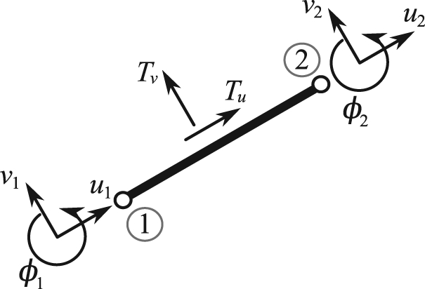
A representative finite element with the corresponding nodal degrees of freedom (u, v, ϕ) subjected to the external traction forces (T_u, T_v) due to the surrounding fluid.

Boundary element formulation of the fluid dynamics equations

For the fluid we make use of the Stokeslet approach in which the force exerted on the fluid at the surface of the solid structure is approximated by the distribution of Stokeslets along the length of the structure. The velocity and force fields are related by a Green’s function that has a singularity proportional to 1/r in three dimensions and ln(r) in two dimensions.²³ The expression of Green’s function (G) for the Stokeslets relates the velocity at location r, $\stackrel{·}{\mathit{u}}$, to the forces at location r′, f, through

$$\stackrel{·}{\mathit{u}}=\mathit{Gf}\hspace{1em}\mathrm{and}\hspace{1em}{G}_{\mathit{ij}}=\frac{1}{4\pi \mu }\{-\ln (R){\delta }_{\mathit{ij}}+\frac{R_i{R}_j}{R^2}\}\hspace{1em}(i,j=1,2),$$ (A9)

where R =r -r′, R = |R| is the distance between the two locations r and r′ and δ_ij is the Kronecker delta. By assuming the point force f to be represented by the traction f =TdS over the solid surface, the boundary-integral equation can be written as

$$\stackrel{·}{\mathit{u}}={\int }_{\mathit{boundary}}\mathit{G}\mathit{T}\mathit{dS}=\sum _{\mathit{nelm}}{\int }_{L_e}\mathit{G}\mathit{T}\mathit{dS}=\sum _{\mathit{nelm}}{\int }_{L_e}\mathit{G}\mathit{N}\mathit{dS}\mathit{t},$$ (A10)

where T are the tractions imposed on the fluid and T = −T_d. In Eq. A10, the boundary-integral equation has been discretized using boundary elements of length L_e, and the tractions are linearly interpolated using T =Nt with t being the tractions at the nodes. When Eq. A10 is used to evaluate the velocity in all nodes of the flagellum, we obtain a system of equations $\stackrel{·}{\mathit{U}}={\mathit{G}}_f\mathit{t}$ that relates the traction t exerted by the flagellum on the fluid to its velocity $\stackrel{·}{\mathit{U}}$. The integration procedure is adopted from the literature.²³ Once the velocity of the solid surface is known, this relation can be inverted to obtain the nodal tractions: $\mathit{t}={\mathit{G}}_f^{-1}\stackrel{·}{\mathit{U}}$.

Fluid-solid interaction and implicit coupling

Coupling of the solid mechanics and fluid dynamics equations will be done in an implicit manner by incorporating the equivalent drag matrix due to the fluid into the stiffness matrix.²⁵ The external nodal force vector due to the fluid’s drag forces (see Eq. A7) can be given as

$${\mathit{f}}_{\mathit{ext}}^{t+\Delta t}={\int }_x{\mathit{N}}^T{\mathit{T}}_d^{t+\Delta t}\mathit{dx}=-{\int }_x{\mathit{N}}^T\mathit{N}\mathit{dx}{\mathit{t}}^{t+\Delta t}=-{\mathit{M}}_e{\mathit{t}}^{t+\Delta t},$$ (A11)

where M_e=∫_xN^TNdx in which we only consider the linear shape functions for N. Note that the minus sign appears due to the change of reference (from fluid to the structure, T_d = –T). After performing the standard finite element assembly procedure we get

$${\mathit{F}}_{\mathit{ext}}^{t+\Delta t}=-{\mathit{Mt}}^{t+\Delta t}=-{\mathit{MG}}_f^{-1}{\stackrel{·}{\mathit{U}}}^{t+\Delta t},$$ (A12)

where the matrix G_f relates the velocity of the solid structure to the traction, see Section 2 of the Appendix. Now, using the no-slip boundary condition $\stackrel{·}{\mathit{U}}=\mathit{A}\Delta \mathit{d}∕\Delta t$ it follows that

$${\mathit{F}}_{\mathit{ext}}^{t+\Delta t}=-{\mathit{MG}}_f^{-1}\mathit{A}\Delta d∕\Delta t=-{\mathit{K}}_D^t\Delta \mathit{d},$$ (A13)

where ${\mathit{K}}_D={\mathit{MG}}_f^{-1}\mathit{A}∕\Delta t$ is an equivalent drag matrix and is the stiffness contribution due to the presence of the fluid. A is a matrix that eliminates the rotational degrees of freedom from the global displacement vector Δd. After incorporating the appropriate boundary conditions, we will be solving the following equation of motion for the FSI problem to obtain the incremental displacements (Δd):

$$\{{\mathit{K}}^t+{\mathit{K}}_D^t\}\Delta \mathit{d}=-{\mathit{F}}_{\mathit{int}}^t.$$ (A14)

References

- Taylor G., Proc. R. Soc. London. Ser. A. Math. Phys. Sci. 209, 447 (1951). 10.1098/rspa.1951.0218 [DOI] [Google Scholar]
- Gray J. and Hancock G. J., J. Exp. Biol. 32, 802 (1955). [Google Scholar]
- Purcell E. M., Am. J. Phys. 45, 3 (1977). 10.1119/1.10903 [DOI] [Google Scholar]
- Becker L. E., Koehler S. A., and Stone H. A., J. Fluid Mech. 490, 15 (2003). 10.1017/S0022112003005184 [DOI] [Google Scholar]
- Dreyfus R., Baudry J., Roper M. L., Fermigier M., Stone H. A., and Bibette J., Nature 437, 862 (2005). 10.1038/nature04090 [DOI] [PubMed] [Google Scholar]
- Lauga E. and Powers T. R., Rep. Prog. Phys. 72, 096601-36 (2009). 10.1088/0034-4885/72/9/096601 [DOI] [Google Scholar]
- Brennen C. and Winet H., Annu. Rev. Fluid Mech. 9, 339 (1977). 10.1146/annurev.fl.09.010177.002011 [DOI] [Google Scholar]
- Tierno P., Golestanian R., Pagonabarraga I., and Sagues F., J. Phys. Chem. B 112, 16525 (2008). 10.1021/jp808354n [DOI] [PubMed] [Google Scholar]
- Ghosh A. and Fischer P., Nano Lett. 9, 2243 (2009). 10.1021/nl900186w [DOI] [PubMed] [Google Scholar]
- Abbott J. J., Peyer K. E., Lagomarsino M. C., Zhang L., Dong L., Kaliakatsos I. K., and Nelson B. J., Int. J. Rob. Res. 28, 1434 (2009). 10.1177/0278364909341658 [DOI] [Google Scholar]
- Khaderi S. N., Baltussen M. G. H. M., Anderson P. D., Ioan D., den Toonder J. M. J., and Onck P. R., Phys. Rev. E 79, 046304 (2009). 10.1103/PhysRevE.79.046304 [DOI] [PubMed] [Google Scholar]
- Khaderi S. N., Craus C. B., Hussong J., Schorr N., Belardi J., Westerweel J., Prucker O., Ruhe J., den Toonder J. M. J., and Onck P. R., Lab Chip 11, 2002 (2011). 10.1039/c0lc00411a [DOI] [PubMed] [Google Scholar]
- den Toonder J., Bos F., Broer D., Filippini L., Gillies M., de Goede J., Mol T., Reijme M., Talen W., Wilderbeek H., Khatavkar V., and Anderson P., Lab Chip 8, 533 (2008). 10.1039/b717681c [DOI] [PubMed] [Google Scholar]
- Holwill M. E. J. and Sleigh M. A., J. Exp. Biol. 47, 267 (1967). [DOI] [PubMed] [Google Scholar]
- Cahill D. M., Cope M., and Hardham A. R., Protoplasma 194, 18 (1996). 10.1007/BF01273164 [DOI] [Google Scholar]
- Brennen C., J. Mechanochem. Cell Motil. 3, 207 (1975). [PubMed] [Google Scholar]
- Kobayashi S., Watanabe R., Oiwa T., and Morikawa H., J. Biomech. Sci. Eng. 4, 11 (2009). 10.1299/jbse.4.11 [DOI] [Google Scholar]
- Fauci L. J., Am. Zool. 36, 599 (1996). [Google Scholar]
- Sleigh M. A., Protoplasma 164, 45 (1991). 10.1007/BF01320814 [DOI] [Google Scholar]
- Woolley D. M., Biol. Rev. 85, 453 (2010). [DOI] [PubMed] [Google Scholar]
- See http://www.jochemnet.de/fiu/bot4404/BOT4404_18.html.
- Higdon J. J. L., J. Fluid Mech. 90, 685 (1979). 10.1017/S0022112079002482 [DOI] [Google Scholar]
- Pozrikidis C., A Practical Guide to Boundary-Element Methods with the Software Library BEMLIB (Chapman & Hall/CRC, Boca Raton, FL, 2002). [Google Scholar]
- Happel J. and Brenner H., Low Reynolds Number Hydrodynamics: With Special Applications to Particulate Media (Springer, New York, 1991). [Google Scholar]
- Khaderi S. N. and Onck P. R., “Implicitly-coupled finite element/boundary element method for the fluid-structure interaction of magnetic artificial cilia” (unpublished).
- Lighthill J., SIAM Rev. 18, 161 (1976). 10.1137/1018040 [DOI] [Google Scholar]
- Dresdner R. D., Katz D. F., and Berger S. A., J. Fluid Mech. 97, 591 (1980). 10.1017/S0022112080002716 [DOI] [Google Scholar]
- See supplementary material at http://dx.doi.org/10.1063/1.3608240E-BIOMGB-5-003103 for an animation of the swept-area by flexible and rigid mastigonemes.
- Sleigh M. A., Metachronism of Cilia of Metazoa, Cilia and Flagella (Academic, London: 1974). [Google Scholar]
- Khaderi S. N., Baltussen M. G. H. M., Anderson P. D., den Toonder J. M. J., and Onck P. R., Phys. Rev. E 82, 027302 (2010). 10.1103/PhysRevE.82.027302 [DOI] [PubMed] [Google Scholar]
- Annabattula R., Huck W., and Onck P., J. Mech. Phys. Solids 58, 447 (2010). 10.1016/j.jmps.2010.02.004 [DOI] [Google Scholar]
- Cook R. D., Malkus D. S., Plesha M. E., and Witt R. J., Concepts and Applications of Finite Element Analysis (John Wiley & Sons, New York, 2002). [Google Scholar]