Abstract
Purpose: In recent years, the authors and others have been exploring the use of penalized-likelihood sinogram-domain smoothing and restoration approaches for emission and transmission tomography. The motivation for this strategy was initially pragmatic: to provide a more computationally feasible alternative to fully iterative penalized-likelihood image reconstruction involving expensive backprojections and reprojections, while still obtaining some of the benefits of the statistical modeling employed in penalized-likelihood approaches. In this work, the authors seek to compare the two approaches in greater detail.
Methods: The sinogram-domain strategy entails estimating the “ideal” line integrals needed for reconstruction of an activity or attenuation distribution from the set of noisy, potentially degraded tomographic measurements by maximizing a penalized-likelihood objective function. The objective function models the data statistics as well as any degradation that can be represented in the sinogram domain. The estimated line integrals can then be input to analytic reconstruction algorithms such as filtered backprojection (FBP). The authors compare this to fully iterative approaches maximizing similar objective functions.
Results: The authors present mathematical analyses based on so-called equivalent optimization problems that establish that the approaches can be made precisely equivalent under certain restrictive conditions. More significantly, by use of resolution-variance tradeoff studies, the authors show that they can yield very similar performance under more relaxed, realistic conditions.
Conclusions: The sinogram- and image-domain approaches are equivalent under certain restrictive conditions and can perform very similarly under more relaxed conditions. The match is particularly good for fully sampled, high-resolution CT geometries. One limitation of the sinogram-domain approach relative to the image-domain approach is the difficulty of imposing additional constraints, such as image non-negativity.
Keywords: computed tomography, sinogram restoration, penalized likelihood, image reconstruction
INTRODUCTION
In recent years, we and others have been exploring the use of penalized-likelihood sinogram-domain smoothing and restoration approaches for emission and transmission tomography.1, 2, 3, 4, 5, 6 The strategy entails estimating the “ideal” line integrals needed for reconstruction of an activity or attenuation distribution from the set of noisy, potentially degraded tomographic measurements by maximizing a penalized-likelihood objective function. The objective function models the data statistics as well as any degradation that can be represented in the sinogram domain. The estimated line integrals can then be input to analytic reconstruction algorithms such as filtered backprojection (FBP). This strategy is, of course, most amenable to modalities such as computed tomography (CT) and positron emission tomography (PET), where the overall imaging equation can, to a good approximation, be decomposed into a transformation representing geometric projection and one or more transformations representing degradations that can be modeled in the data domain. In modalities such as single-photon emission computed tomography (SPECT), the depth-dependent attenuation likely prevents this kind of factorization.
The motivation for this strategy was initially pragmatic: to provide a more computationally feasible alternative to fully iterative penalized-likelihood image reconstruction involving expensive backprojections and reprojections, while still obtaining some of the benefits of the statistical modeling employed in penalized-likelihood approaches. We viewed the approach as a potential middle ground between the use of fully iterative, statistically principled algorithms on the one hand and more efficient analytic algorithms that neglect data statistics on the other.
However, in this work, we show that, under certain conditions, the approaches satisfy the conditions for equivalent optimization problems and thus produce identical reconstructed images (Ref. 7, Sec. 4.1.3). A related proof has been given previously by August using a continuous-domain formulation.8 Here we focus on the discrete formulation that is generally the starting point for the derivation of iterative algorithms. While restrictive in practice, these conditions do provide guidance on mapping objective functions between the two domains, which is particularly useful for mapping of penalty functions. We show that a local penalty in the image-domain maps to a fairly local penalty in the sinogram that we further approximate to reduce computational burden. Using this approximate penalty and an approximate inverse of the tomographic projection transform (provided by the FBP algorithm), we show using brute force and analytic calculations that the sinogram-domain approach can produce extremely similar resolution-variance tradeoffs as the image-domain approach when applied to the simple transmission tomography imaging equation, which is the most likely realm of application of the strategy. The match is particularly good for fully sampled, high-resolution CT geometries. The sinogram-domain approach cannot, at present, correct for artifacts caused by inaccuracies of the system model or incompleteness of the data sampling, such as the conebeam artifacts caused by the use of approximate reconstruction algorithms or by the use of inadequate illumination trajectories (such as a circular conebeam acquisition).
In Sec. 2, we lay out the problem and then present the conditions for the equivalence of the image- and sinogram-domain methods. We show how these conditions, while restrictive, can be used in practice to map penalties between the image and sinogram domains. In Sec. 3, we summarize the methods used for comparing the two approaches, including the use of simulation and analytic tools to assess image quality. The results of the evaluations and conclusions are presented in Secs. 4, 5, respectively.
METHODS
In this section, we set up the class of imaging equations to be considered and define appropriate objective functions in the image and sinogram domains. We then present the conditions for the equivalence of the image- and sinogram-domain methods. While restrictive, these conditions provide a framework for mapping penalty functions between the two domains, which is discussed at the end of the section.
Imaging equations
For a number of tomographic imaging modalities, the discrete-to-discrete imaging equation can, to a good approximation, be decomposed into a matrix representing geometric projection between the image domain and data domain and one or more matrices or transformations representing operations or degradations that can be modeled in the data domain.
For example, consider a discrete representation of an object as an N-dimensional vector x and let P be an M × N matrix representing tomographic projection of the object into an M-dimensional sinogram space. For simplicity, we refer to
| (1) |
as the set of line integrals of the object, though the matrix P need not be a simple discretization of the Radon transform but could model more accurately the geometry of the projection operation (such as uniform attenuation and depth-dependent blurring in single-photon emission computed tomography, which can be modeled and inverted analytically9). Many imaging equations can then be expressed generally in terms of the line integrals as
| (2) |
where is an M-dimensional mean data vector and g is a function from RM to RM. We consider now some specific imaging equations for emission and transmission tomography.
Emission tomography
Some emission tomography modalities yield a mean data vector that can be modeled as
| (3) |
where B is an M × M matrix that captures effects that can be modeled in the sinogram domain. For instance, Leahy and Qi have modeled PET data in this way,10 where the matrix B represents data-space effects such as attenuation, detector blur, and detector sensitivity (to match Leahy and Qi’s model exactly, the effect of positron range could also be included in the matrix P along with geometric projection). This imaging equation has the form of Eq. 2 with g(z) = Bz.
Overall, then, this imaging equation can be written as
| (4) |
where the overall system matrix is given by
| (5) |
Transmission tomography
In transmission tomography, the most basic but still important model connecting the line integrals to the measured data simply involves an exponential operation. The mean data vector then has elements
| (6) |
where Ii is the intensity of the incident x-ray beam along the ith line integral and zi is the ith element of z from Eq. 1
| (7) |
Equation 6 has the form of Eq. 2 with gi(z)=Iie-zi.
In practical CT scanners, there are often nonidealities in the data-acquisition process such as off-focal radiation, crosstalk, and beam hardening.11 We have developed a CT model in which the measurements are given by
| (8) |
where the Cij model “contamination” among ideal line integral measurements by, for example, crosstalk, afterglow, and off-focal radiation, while the functions fj(zj) model mismapping of line-integral values due to the polychromatic spectrum and beam hardening.5 Equation 8 has the form of Eq. 2 with .
Image- and sinogram-domain penalized-likelihood algorithms
In practice, the data measured in any real scanner is further contaminated by noise governed by a statistical density f(y;x), which in most cases is modeled as either Poisson or Gaussian. In recent years, many investigators have demonstrated the advantages of accurate modeling of data statistics in the context of image reconstruction (see Refs. 12, 13 and references contained therein). This is most commonly done through the use of maximum-likelihood or penalized-likelihood algorithms, which are generally implemented in the image domain (direct estimation of the image of interest) but occasionally in the sinogram domain (direct estimation of “ideal” line integrals followed by analytic image reconstruction).1, 2, 3, 4, 5, 6 In this section, we introduce these two approaches and then explore the conditions under which they are actually mathematically equivalent. While somewhat restrictive in practice, these conditions do provide a way of mapping objective functions between the two domains, which is particularly useful for mapping of penalty functions.
Image-domain penalized-likelihood algorithms
In image-domain penalized-likelihood algorithms, one seeks to find the solution that maximizes a predefined objective function comprising two competing terms that reward agreement with the measured data and penalize roughness, respectively. The superscript PL–I denotes the image-domain penalized-likelihood estimator. For example
| (9) |
where
| (10) |
Here, L (x | y) is the statistical likelihood or log-likelihood function and Rx(x) is a penalty function, with β the smoothing parameter that determines the relative influence of the two terms. Further constraints on x are sometimes added to the optimization problem, most commonly non-negativity. The solution to the optimization problem is almost always found iteratively. This is so even in the rare cases when the optimization problem has a closed-form solution, owing to the large dimensionality of the problem.
It is important now to consider the concavity of the objective functions, since concavity implies the existence of a unique maximizer and has implications for the connections between the image- and sinogram-domain approaches to be explored in Sec. 2B3. For a convex penalty function and a concave log-likelihood function, the overall objective function is concave (the negative sign in front of the penalty term makes it concave, and the non-negative sum of two concave functions is concave7). It is straightforward to show that the log-likelihood function is concave for both Poisson and Gaussian noise models applied to either the emission tomography or simple transmission tomography imaging equations.12 The degraded transmission tomography model of Eq. 8 does not, in general, yield a concave log-likelihood for either noise model though in practice we have found that it converges to a reasonable local maximum given a reasonable starting guess.
Sinogram-domain penalized-likelihood algorithm
Consider a second, sinogram-domain, strategy, in which we estimate “ideal” line integrals by solving
| (11) |
using a penalized-likelihood strategy, such that
| (12) |
for an appropriately chosen objective function Φz (z). We then estimate the image by applying a discretized analytic reconstruction algorithm whose action we represent by the operator O
| (13) |
The intent is that the matrix O ≈ P−1. Here, the superscript PL–S denotes the sinogram-domain penalized-likelihood estimator. The advantages of this approach are generally computational. In general, finding the maximizing Eq. 12 is much less computationally intense than finding the maximizing Eq. 9 since the degradations it models are generally relatively local operations in the sinogram domain rather than backprojections and reprojections.
Conditions for the equivalence of the image- and sinogram-domain approaches
Perhaps surprisingly, the image- and sinogram-domain strategies are equivalent under certain conditions. When these conditions hold, the two approaches become so called equivalent optimization problems [Ref. 7, Sec. 4C]. The conditions are
-
(1)
The objective function Φx(x) is concave and thus has a unique maximum.
-
(2)
The projection matrix P is invertible and the inverse P−1 is known.
-
(3)The objective function Φz(z) is constructed as
so that(14) (15) -
(4)
We use P−1 to reconstruct the idealized line integrals
| (16) |
If these conditions hold, then
| (17) |
This follows because P represents an invertible mapping (a coordinate transformation, in a sense) between the unique maximizers and . It should be noted that the treatment of equivalent optimization problems is even more general than given above in that it also accommodates equality and inequality constraints, appropriately mapped between the two spaces [Ref. 7, Sec. 4.1.3]. We have not explored the use of such constraints since a simple image-domain constraint such as non-negativity can map to a complicated sinogram-domain constraint, which could undermine the computational advantage of the sinogram-domain approach.
Practical use for penalty mapping
The conditions for the precise equivalence of the image- and sinogram-domain approaches are obviously quite restrictive and unlikely to be exactly satisfied in practice. The matrix P−1 may not exist or be readily calculable. However, as we will explore below, the sinogram-domain approach can produce extremely similar results to the image-domain approach even when we have only an approximation of P−1 provided by an analytic algorithm such as FBP. Achieving this similar performance depends on using the correct sinogram-domain objective function and specifically the correct penalty, which can be obtained from the expression for mapping objective functions between the domains given in Eq. 14. This formula provides a recipe for calculating the penalty to apply in the sinogram domain when a given image-space penalty is specified
| (18) |
For example, if the image-space penalty is quadratic, Rx(x) = xTRIx, then the penalty to be applied in the sinogram space will be R(z) =zTRSz, where RS ≡ (P−1)TRIP−1.
In practice, we do not need to assume that we have a closed-form expression for P−1 to perform the penalty mapping. If all we have is a discretized analytic image reconstruction algorithm such as FBP, whose action we represent by the matrix O ≈ P−1, we can use it to evaluate the elements of the sinogram-domain penalty
| (19) |
For the quadratic case, the jk component of RS can be found by evaluating
| (20) |
where the vector z(j) denotes a vector in the space z in which only element j, which is set equal to 1, is nonzero. (In other words, it is a sinogram with only one nonzero line integral.) This can be evaluated as follows:
-
(1)
Perform image reconstruction on z(k) to evaluate Oz(k)
-
(2)
Act on the resulting image with RI.
-
(3)
Finally, take inner product with Oz(j), also obtained by reconstructing z(j)
An example of penalty mapping
To examine how penalties map between domains, we evaluated the sinogram-domain penalty corresponding to a quadratic image-domain penalty with matrix RI constructed to penalize differences between a given pixel and its four nearest neighbors (horizontal and vertical) in a 642 pixel image using Eq. 20. We did so for both parallel-beam and fanbeam geometries. Images of the resulting RS matrices are shown in Fig. 1 with a very tight display window (between 0 and 5% of the maximum) in order to emphasize the structure of the matrix. The prominent diagonal line corresponds to a given channel’s own contribution to the assessment of the penalty. Of greatest interest in these figures is the energy dispersed on diagonal lines about halfway toward the top left and bottom right corners. These correspond to conjugate rays of the diagonal and its neighboring channels. This can be seen more clearly in the line profiles through the matrices shown in Fig. 2, where one observes, not surprisingly, that the contribution of a given ray and its neighborhood to the sinogram-domain penalty is mirrored by that of the conjugate ray and its neighborhood.
Figure 1.
Matrices RS for parallel (left) and fanbeam (right) geometries. The prominent diagonal line corresponds to a given channel’s own contribution to the assessment of the penalty. The energy in the bands midway to the corners corresponds to contributions of the conjugate rays.
Figure 2.
Typical line profiles through the penalty matrix for parallel (left) and fanbeam (right) geometries. The pair of spikes corresponds to contributions of the ray of interest and of its conjugate partner.
For a selected j, we plot RS,jk for a range of k corresponding to three projection views in Fig. 3. The central feature corresponds to coefficients applied to the nearest channel neighbors of channel j within the same projection. The smaller peripheral features correspond to coefficients applied across projection views and they are also centered around channel j.
Figure 3.
Plot of RS,jk for a fixed j for a range of k corresponding to about three projection views.
A zoomed view of the central feature seen in Fig. 3, which corresponds to coefficients applied to the neighboring detector bins in the same projection view as j, is shown in Fig. 4.
Figure 4.
Plot of RS,jk for a fixed j for a range of k corresponding to about ten channels on either side of j. This is a zoomed view of the central feature in Fig. 3.
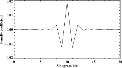
Because the computational burden of applying the sinogram-domain penalty increases with the number of coefficients in the penalty matrix, we investigate in the rest of this paper using an approximate version of the sinogram-domain penalty that is simply a neighborhood differencing penalty applied to the difference of bin j with its two nearest bin neighbors. The coefficients are shown in Fig. 5, and they can be seen to provide a reasonable approximation of the central feature of the exact sinogram-domain penalty.
Figure 5.
Plot of the approximate RS,jk we employ for a fixed j for a range of k corresponding to about ten channels on either side of j.
METHODS FOR COMPARING IMAGE- AND SINOGRAM-DOMAIN APPROACHES
Our aim in the remainder of this paper is to compare the performance of the image- and sinogram-domain methods for the simple transmission tomography model of Eq. 6. This is a case for which comparable iterative algorithms exist in the two domains. Ultimately, we would like to compare the image- and sinogram-domain approaches for the degraded CT model of Eq. 8. However, most fully iterative approaches to CT reconstruction do not model any sinogram-domain degradations, but actually begin with precorrected, calibrated, logged data, so it not possible to make a direct comparison between image- and sinogram-domain approaches to solving Eq. 8 without first developing a new class of algorithms.
We compare the resolution and noise properties of the two approaches, and specifically the resolution and noise tradeoffs, by calculating the local impulse response function and variance at a variety of points in a phantom. Our methods for evaluating these are described below in Secs. 3A, 3B. We simulate Poisson noise (plus a small Gaussian electronic noise) and use the Poisson log-likelihood function in the objective
where
| (21) |
We employ a quadratic penalty based on the difference of the four nearest pixel neighbors in the image domain. In the sinogram domain, we use the approximate mapped penalty based on the simple quadratic difference of a sinogram bin with its nearest neighbors. For image-domain reconstruction, we use an iterative update derived by Erdogan and Fessler based on the separable paraboloidal surrogates strategy that is guaranteed to increase the objective function at every iteration with appropriate choice of parabola curvatures.14 We use the fast precomputed curvatures they propose that do not guarantee monotonicity but monitor the objective function for nonpositive steps. If any occur, we repeat the iteration with a guaranteed monotonic choice of curvature (in practice, this never happened). This algorithm naturally enforces non-negativity in the estimated image. In the sinogram-domain, we use the same algorithm with the projection matrix set to the identity matrix as we have previously described.4 Filtered backprojection with an unapodized ramp filter is used for image reconstruction from the estimated line integrals. This algorithm naturally enforces non-negativity of the estimated line integrals (which does not necessarily imply non-negativity in the reconstructed image).
Local impulse response
A local impulse response (LIR) function is a generalization of a point spread function to a shift-variant, potentially nonlinear imaging system. It describes the response of the system to an impulse placed at a particular point in a particular object. For an estimator with mean , the local impulse response of the jth pixel is defined to be
| (22) |
Here is the estimated image obtained from data corresponding to the impulse-containing object xImp–j = x + δej, where δej is a small impulse placed in the jth pixel.
Brute force evaluation of local impulse response
Most estimators do not have an explicit analytical form. Thus, one natural approach to evaluating the local impulse response is the following brute-force approach: (1) Select an object x of interest and generate multiple realizations of noisy measurements according to the density f(y; x). (2) Apply the estimator of interest to each of the measurement realizations to obtain estimates and average these to estimate the sample mean. (3) Choose a pixel j of interest and small value δ and generate a second set of noisy measurements according to the density f (y; xImp). (4) Compute the sample mean of the second set and subtract the two sample mean images (with and without the impulse) to obtain an estimate of the local impulse response.
Approximate analytic evaluation of local impulse response
While effective, the brute-force approach quickly becomes computationally prohibitive for problems of large dimension. Fortunately, Fessler derived approximate analytic expressions for LIR in transmission CT.15 We will validate these by comparing to brute-force approaches for smaller-dimensioned problems in order to license their use for the matrix sizes of interest. Fessler’s expression for the image-domain estimate is given by
| (23) |
where
| (24) |
We show in Appendix A that a very similar expression can be described for the sinogram-domain approach
| (25) |
This estimation of the local impulse response is desirable since it is independent of the PL estimate of the image and depends only on the noiseless data.
To summarize the spread in a given LIR, an average full width at half-maximum (FWHM) metric was calculated with the following procedure. The value and index of the highest intensity pixel were recorded. The index location of the pixels immediately above and below the half-maximum value along the x and y-axes were recorded. The half-max locations were calculated by linear interpolation of these pixels and used to calculate the full-width for the x- and y-axes. Since PL approaches may produce local impulse responses that are anisotropic, impulse profiles were measured at 1° intervals and averaged together. The impulse profiles were taken from the impulse image rotated and rebinned using bilinear interpolation. Additionally, all of the pixels along these profiles were confirmed to be monotonically decreasing and greater than zero ensuring there was no undershoots or overshoots in the LIR. Note that because the impulse is the size of a pixel rather than infinitesimal, the true system resolution (response to an infinitesimal impulse) is actually one pixel smaller than is measured from the FWHM of the LIR.
Variance and covariance
Brute force evaluation of covariance
Again, when there is no explicit form for , there is usually no explicit form for the estimator variance either, and a brute-force numerical approach becomes a natural option: (1) Select an object x of interest and generate multiple realizations of noisy measurements according to the density f (y; x). (2) Apply the estimator of interest to each of the measurement realizations. (3) Estimate the estimator sample covariance.
Approximate analytic evaluation of variance
As with LIR, Fessler has derived approximate analytic expressions for the covariance of PL transmission tomography reconstruction. For a quadratic penalty, we have
| (26) |
In the sinogram domain, we show in Appendix A that the covariance matrix is given by
| (27) |
In the resolution-variance plots below, we assess the variance at the pixel whose LIR is used for the resolution measure.
Simulation studies
For all resolution-variance studies, we used the 1024 × 1024 attenuation image shown in Fig. 6, which has linear attenuation coefficients of 0.130, 0.096, and 0.030 cm−1 in the hot disk (left), background ellipse, and cold disk (right), respectively. The pixel size was .0375 cm. The background ellipse has a major axis of 34.54 cm and minor axis of 19.2 cm, while the hot and cold disks have 11.52 cm diameters. To examine the performance of the proposed penalized-likelihood algorithms, we simulated both noisy and noiseless projections of this numerical phantom. For parallel-beam data, we computed a sinogram of 1024 parallel bins of extent .0375 cm at the isocenter by 1024 angles acquired over 360°. We did not employ a quarter detector offset. We simulated the data using a monochromatic spectrum at the average energy . We exponentiated and rebinned this large sinogram into smaller-dimensioned sinograms in order to perform computationally intensive tasks like brute-force evaluation of variance. For the clinically realistic fanbeam data, we used the Radonis CT simulation package (Philips R&D, Hamburg) to simulate a typical 672 channel by 1160 angle acquisition.
Figure 6.
Numerical ellipse phantom used to determine image properties.
We reconstructed the images using several combinations of smoothing and analytic reconstruction. The sinogram-domain algorithm was applied with 31 beta parameters β chosen to span an appropriate resolution range and then image reconstruction was performed with FBP using an unapodized ramp filter. The image-domain algorithm was used to reconstruct images at 31 different β values chosen to span the same range of resolution (the beta values in the sinogram- and image-domain approaches differ by a factor approximately equal to N for N × N images, a fact that follows from the penalty-matching formalism). FBP using the Hanning filter with Nyquist cutoff was used as the initial guess. All iterative algorithms were run to 500 iterations to unequivocally ensure convergence. In practice, the sinogram-domain algorithm often converged within approximately ten iterations and the image-domain within about 100 iterations for the lower beta values corresponding to the resolutions of greatest diagnostic interest, as judged by monitoring the objective function and LIR and variance values.
Validating the penalty-matching strategy
To confirm that this appropriate choice of sinogram-domain roughness penalty can match the properties and performance of a given image-domain penalty, we generated parallel-beam 512 bin × 512 angle transmission tomography sinograms of the phantom shown in Fig. 6 and reconstructed onto a 512 × 512 array. The exposure was 1 × 10⁵ incident counts per channel. We used penalized-likelihood methods to calculate noisy images and local impulse response functions for three different reconstruction approaches: the image-domain approach with a quadratic first-order neighborhood penalty, the sinogram-domain approach with the penalty calculated by Eq. 20, and the sinogram-domain approach with the approximate penalty corresponding to a first-order channel neighborhood.
Parallel-beam resolution-variance studies for square system matrix
We performed resolution-variance studies, first for the case of a square system matrix. We performed brute-force evaluations of variance and LIR for the 128 × 128 problem size by generating and reconstructing 2000 realizations. The purpose was to validate the use of the analytical approximations for the larger nonsquare problem sizes. When creating noisy sinograms, Poisson statistics were used on the resized sinogram. We also added electronic noise with variance equivalent to the counting statistics variance of ten detected photons. We used exposures 1 × 10⁴, 1 × 10⁵, and 1 × 10⁶.
Parallel-beam resolution-variance studies for nonsquare system matrix
To explore the situation where the matrix P is not square and thus cannot have a unique inverse, we repeated the above studies for both overdetermined systems where there are more measurements than unknowns, which is typically the case in CT, and also an underdetermined system in which there are more unknowns than measurements. For the overdetermined system, we simulated 256 bin × 384 angle and 256 bin × 512 angle sinograms, with reconstruction on a 256 × 256 pixel grid. This was to study the situation typical in CT where the angular sampling exceeds the radial sampling by different ratios. For the underdetermined system, we simulated 128 bin × 128 angle sinograms and reconstructed on a 256 × 256 grid.
Fanbeam resolution-variance and anatomical phantom studies for clinically typical geometry
We also sought to verify that the algorithms work comparably on a more clinically realistic fanbeam geometry with both the resolution-variance phantom and a complex, anatomically realistic phantom. We conducted the anatomical study by reprojecting two CT reconstructions of a patient shoulder and abdominal slice using the Radonis CT simulation package (Philips R&D, Hamburg). We modeled a single-slice detector array of 672 channels of total extent 946 mm, with a focal length of 570.0 mm. A total of 1160 projections over 360° were simulated. We then added noise as described in Sec. 3C2. For the resolution-variance studies, the data sizes were too large to allow use of either the analytic method or the use of thousands of noise realizations. So we reconstructed single realizations of noiseless data with and without the presence of an impulse in order to assess the LIR as well as single realizations in the presence of noise to asses the variance properties. The variance was measured as the sample variance of a small ROI centered around the cold, hot, and background disks in the resolution-variance phantom. For the anatomical phantoms, we chose beta values to produce matched resolution as determined by studying profiles through small, intense objects, such as an enhanced blood vessel. Reconstruction was performed with 0.75 mm pixels.
Computational comparison
We ran the sinogram- and image-domain algorithms on a 256 bin × 256 angle sinogram reconstructed onto a 256 × 256 pixel array on a MacPro, a MacMini, a Dell Workstation running Linux, and a Xeon-based cluster and calculated average per iteration computation times for each of the two approaches.
RESULTS
Validating the penalty-matching strategy
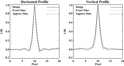
Typical noisy images for exposure 1 × 10⁵ are shown in Fig. 7, and they are qualitatively similar. The local impulse responses measured in the hot circle are shown in Fig. 8. The shape and width for all three are seen to be extremely similar, which is confirmed by the horizontal and vertical profiles through the LIRs shown in Fig. 9.
Figure 7.
Typical noisy images for (left) image-domain penalty (center) “exact” sinogram-domain penalty (right) approximate sinogram-domain penalty.
Figure 8.
Local impulse responses in the hot circle for (left) image-domain penalty (center) “exact” sinogram-domain penalty (right) approximate sinogram-domain penalty.
Figure 9.
Horizontal (left) and vertical (right) profiles through the LIRs for image domain, exact sinogram domain, and approximate sinogram domain.
Parallel-beam resolution-variance studies for square system matrix
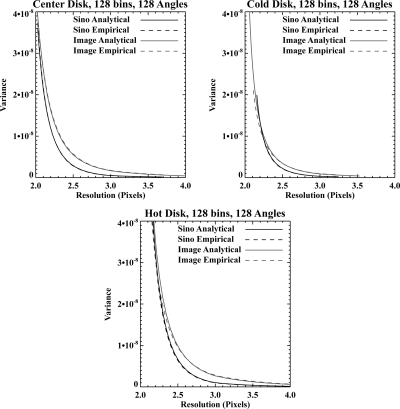
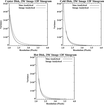
The resolution-variance results for the 128 × 128 images at exposure level 1 × 10⁶ are shown in Fig. 10. The results at other exposure levels are essentially identical, with all the variance values shifted upward by an appropriate factor, so we only show the 1 × 10⁶ results in the interest of space. We show results calculated using both the brute-force approach (“empirical”) and the analytic expressions for both the sinogram- and image-domain approaches. We see from the figure that the agreement between the empirical and analytical results is excellent, which licenses the use of the analytic expression for larger problems where calculating hundreds of realizations is not feasible. We also see that the resolution-variance tradeoffs achieved by the sinogram-domain are generally better than those achieved by the image-domain approach, except in the highest resolution realm for the cold disk, where the curves cross. Because of the use of the approximate penalty, the resolution variance was not necessarily expected to be identical, and it is encouraging that the sinogram-domain approach outperforms the image-domain in this situation.
Figure 10.
Square system matrix: resolution-variance tradeoffs for points at the center of the phantom and at the center of the “hot” and “cold” disks for reconstruction of a 128 × 128 image from a 128 bin × 128 angle sinogram. We show results calculated using both the brute-force approach (“Empirical”) and the analytic expressions (“Analytical”) for both the sinogram- and image-domain approaches.
Parallel-beam resolution-variance studies for nonsquare system matrix
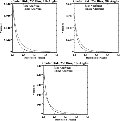
The results for the overdetermined nonsquare system matrix are shown in Fig. 11. The resolution-variance tradeoff at the center of the phantom is shown for 256-, 384-, and 512-angle sinograms. The results are similar to those seen for the square system matrix, indicating that the method is not dependent on the system matrix being square and potentially invertible. However, we note that as the number of angles increases, the resolution-variance curves cross, with the image-domain approach showing an advantage at very high resolutions. This is likely a consequence of the fact that we are using an approximate sinogram-domain penalty that does not apply the penalty between angles. While this was a good approximation to the more exact penalty for sparser angular sampling, it may not be as good for the denser sampling.
Figure 11.
Overdetermined system matrix: resolution-variance tradeoffs for points at the center of the phantom for reconstruction on a 256 × 256 grid from sinograms of 256 bins and 256, 384, and 512 angles.
The results for the underdetermined system are shown in Fig. 12. They are extremely similar to the results shown for square system matrices, indicating that the penalty-mapping approximation does not break down immediately in the case of underdetermined linear systems.
Figure 12.
Underdetermined system matrix: resolution-variance tradeoffs for points at the center of the phantom and at the center of the “hot” and “cold” disks for reconstruction of a 256 × 256 image from a 128 bin × 128 angle sinogram. Despite the problem being underdetermined, both image-domain and sinogram-domain approaches still perform similarly.
Fanbeam resolution-variance and anatomical phantom studies for clinically typical geometry
The results of the resolution-variance studies for the clinically realistic fanbeam geometry are shown in Fig. 13. The sinogram-domain and image-domain curves align nearly perfectly, indicating that the image- and approximate sinogram-domain methods are comparable for clinically realistic fanbeam geometries as well as for the parallel-beam geometries we have considered.
Figure 13.
Resolution-variance tradeoffs for points at the center of the cold and hot disks and at the center of the phantom for reconstruction of an image from a 672 bin × 1160 angle fanbeam sinogram. Pixel size is 0.75 mm.
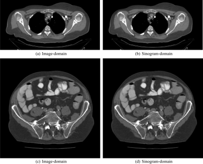
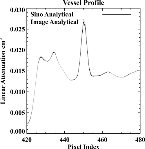
The anatomical images are shown in Fig. 14. The images are seen to be extremely similar. To match resolution, we looked at profiles through small enhanced vessels, as shown in Fig. 15. Typical profiles are shown in Fig. 16.
Figure 14.
Reconstructed images of shoulder and abdomen slices using the image- and sinogram-domain approaches. Resolution has been matched between each pair of images by comparing profiles, as shown in Fig. 16. (Window = 100, Level = 0).
Figure 15.
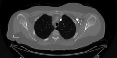
Shoulder phantom showing where the profiles were examined for resolution matching (along the three small white lines shown to the right of the lung) and where the noise was sampled in a relatively uniform ROI (near the upper left).
Figure 16.
Profile through the bright enhanced vessel in the shoulder slice showing that resolution has been well matched between the images reconstructed by the image- and sinogram-domain approaches.
Noise was measured by calculating the standard deviation in the small, uniform ROI depicted in Fig. 15 and found to be 0.00015 cm−1 for the image-domain approach and 0.00014 cm−1 for the sinogram-domain approach, again indicating extremely similar performance under matched conditions.
Computational comparison
The results of the computational comparison were that the sinogram-domain method took an average of 0.033 s per iteration while the image-domain method took an average of 0.32 s per iterations; this was consistent across all five machines. In addition to this ten-fold higher per iteration computational burden, the image-domain approach generally requires ten times more iterations to converge than the sinogram-domain approach, though the exact number is object and smoothing-parameter dependent. Overall, the sinogram-domain approach runs approximately two orders of magnitude faster.
DISCUSSION AND CONCLUSIONS
We have considered a class of tomographic imaging equations that can, to a good approximation, be decomposed into a transformation representing geometric projection between the image domain and data domain and one or more transformations representing operations or degradations that can be modeled in the data domain. We indicated that for such imaging equations, in addition to the usual fully iterative penalized-likelihood image reconstruction approaches, one can also pursue a sinogram-restoration strategy. In this case, the sinogram-domain degradations are corrected using a penalized-likelihood strategy and then the resulting “ideal” line integrals are input to analytic image reconstruction algorithms.
We have shown that under certain conditions, the approaches satisfy the conditions for equivalent optimization problems and thus produce identical reconstructed images. These conditions are that (1) the objective function is concave, (2) the projection matrix P is invertible and the inverse P−1 is known, (3) the sinogram-domain objective function is appropriately constructed from the image-domain objective and knowledge of P−1, and (4) P−1 is used to reconstruct the idealized line integrals.
While restrictive in practice, these conditions do provide guidance on mapping objective functions between the two domains, which is particularly useful for mapping of penalty functions. We showed that a local penalty in the image-domain maps to a fairly local penalty in the sinogram that we further approximated to reduce computational burden. Using this approximate penalty and an approximate inverse of P (provided by the FBP algorithm), we showed that the sinogram-domain approach can produce extremely similar resolution-variance tradeoffs as the image-domain approach when applied to the simple transmission tomography imaging equation. These comparisons were made both using brute-force methods involving multiple noise realizations, for small-dimensioned problems, and using approximate analytic expressions for noise and resolution properties of implicit estimators, for larger problems. The analytic methods were validated against the brute-force results for the smaller problems.
There are, naturally, limits to what can be accomplished simply through sinogram restoration rather than through fully iterative image-domain reconstruction. As discussed earlier, constraints such as non-negativity that are very simple to enforce in the image domain may be hard to enforce in the sinogram domain. While the equivalent optimization formalism provides a way of mapping such constraints between domains, the constraints would likely take a complex form in the sinogram domain that would undermine the simplicity and computational efficiency of the approach. Likewise, highly space-variant penalties that are tuned to particular features in image space may be difficult to implement efficiently in the sinogram domain. Finally, while it might be possible to correct or at least compensate for these effects in the future, the sinogram-domain approach cannot, at present, correct for artifacts caused by inaccuracies of the system model or incompleteness of the data sampling.
Natural future extensions of the work presented here would explore these issues. Close examination of the fanbeam penalty matrix shows that while the structure of the coefficients appears to be shift-invariant to a high degree, the overall magnitude of the coefficients falls off somewhat as one moves toward peripheral channels at a given view angle. This suggests that a kind of spatially variant smoothing may be optimal in the fanbeam case, with less penalizing of roughness towards the peripheral channels, which might compensate for the tendency of fanbeam images to suffer loss of resolution at the edge of the field of view. Our preliminary efforts to incorporate this into our approximate penalty did not show any noticeable advantage, but we will continue to pursue this direction.
We also plan to investigate the application of the penalty mapping strategy to more complicated, nonquadratic penalties as well as to explore techniques for producing optimal factorizations and decompositions of imaging equations to exploit this strategy. For instance, in the case of negligible attenuation, it appears that the SPECT system matrix, which is dominated by depth-dependent resolution effects, could be represented by a factorization that models the depth-dependent resolution as a blurring in sinogram space, much as we have done in modeling the effect of anode angulation in CT.16
ACKNOWLEDGMENT
This work was supported in part by NIH Grant No. R01CA134680.
APPENDIX: derivation of lir and covariance
We present here the derivation of the LIR and covariance expressions for the sinogram-domain penalized-likelihood approach. The LIR is defined to be
| (28) |
For the sinogram-domain approach, we have
| (29) |
where
| (30) |
Here we have made explicit the dependence of the objective function on the measured data vector. It is given by
| (31) |
Plugging Eq. 29 into Eq. 28 and exchanging the linear reconstruction operator and derivative yields
| (32) |
The derivative with respect to the mean maximizer of Eq. 30 can be evaluated using the method of Fessler that exploits the implicit function theorem and the chain rule.17 The result given there is that
| (33) |
where
| (34) |
| (35) |
and where is the result of applying the estimator to noiseless data . The derivative of the noiseless data function
| (36) |
which yields
| (37) |
where D denotes a diagonal matrix and ej is a unit vector.
For a Poisson log-likelihood, we have
| (38) |
Focusing on the derivatives of the likelihood term, we find
| (39) |
where D denotes a diagonal matrix and
| (40) |
where I denotes the identity matrix. Assuming a quadratic penalty Rz(z) =zTRSz, we have ∇20Rz(z) = RS. Substituting all of these results into Eq. 33 yields
| (41) |
where we have used .
The derivation of the covariance expression is even more straightforward. The covariance matrix for the estimate of follows directly from the covariance estimate for since the objective function has exactly the same form, only with the projection matrix P being absent (i.e., replaced with the identity matrix) and with Rz in place of Rx in the penalty term. So we find
| (42) |
Since
| (43) |
then by the usual rules for transformation of random vectors, we have
| (44) |
This is a greatly expanded and revised version of a conference proceedings paper from the 1st International Meeting on Image Formation and Reconstruction in CT.
References
- Fessler J. A., “Tomographic reconstruction using information-weighted spline smoothing,” in Information Processing in Medical Imaging, edited by Barrett H. H. and Gmitro A. F.Springer-Verlag, Berlin, 1993, pp. 290–300. [Google Scholar]
- La Rivière P. J. and Pan X., “Nonparametric regression sinogram smoothing using a roughness-penalized poisson likelihood objective function,” IEEE Trans. Med. Imaging 19, 773–786 (2000). 10.1109/42.876303 [DOI] [PubMed] [Google Scholar]
- La Rivi P. J.ère and D. M. Billmire, “Reduction of noise-induced streak artifacts in x-ray computed tomography through penalized-likelihood smoothing,” IEEE Trans. Med. Imaging 24, 105–111 (2004). 10.1109/TMI.2004.838324 [DOI] [PubMed] [Google Scholar]
- La Rivi P. J.ère, “Penalized-likelihood sinogram smoothing for low-dose CT,” Med. Phys., Ann Arbor, MI 32, 1676–1683 (2005). 10.1118/1.1915015 [DOI] [PubMed]
- La Rivi P. J.ère, J. Bian, and P. Vargas, “Penalized-likelihood sinogram restoration for computed tomography,” IEEE Trans. Med. Imaging 25, 1022–1036 (2006). 10.1109/TMI.2006.875429 [DOI] [PubMed] [Google Scholar]
- Li T., Li X., Wang J., Wen J., Lu H., Hsieh J., and Liang Z., “Nonlinear sinogram smoothing for low-dose X-ray CT,” IEEE Trans. Nucl. Sci. 51, 2505–2513 (2004). 10.1109/TNS.2004.834824 [DOI] [Google Scholar]
- Boyd S. and Vandenberghe L., Convex Optimization (Cambridge University Press, Cambridge, 2004). [Google Scholar]
- August J., “Decoupling the equations of regularized tomography,” in Proceedings of the 2002 IEEE International Symposium Biomedical Imaging, (IEEE, Piscataway, New Jersey, 2002), pp. 653–656. [Google Scholar]
- Pan X., “Analysis of 3D SPECT image reconstruction and its extension to ultrasonic diffraction tomography,” IEEE Trans. Nucl. Sci. 45, 1308–1316 (1998). 10.1109/23.682022 [DOI] [Google Scholar]
- Leahy R. and Qi J., “Statistical approaches in quantitative positron emission tomography,” Stat. Comput. 10, 147–165 (2000). 10.1023/A:1008946426658 [DOI] [Google Scholar]
- Hsieh J., Computed Tomography: Principles, Design, Artifacts, and Recent Advances, SPIE, Bellingham, 2003. [Google Scholar]
- Fessler J. A., “Statistical image reconstruction methods for transmission tomography,” in Handbook of Medical Imaging, Volume 2, edited by Fitzpatrick J. M. and Sonka M.SPIE, Bellingham, WA, 2000, pp. 1–70. [Google Scholar]
- Qi J. and Leahy R. M., “Iterative reconstruction techniques in emission computed tomography,” Phys. Med. Biol. 51 (15), R541–R578 (2006). 10.1088/0031-9155/51/15/R01 [DOI] [PubMed] [Google Scholar]
- Erdogan H. and Fessler J. A., “Monotonic algorithms for transmission tomography,” IEEE Trans. Med. Imaging 18, 801–814 (1999). 10.1109/42.802758 [DOI] [PubMed] [Google Scholar]
- Fessler J. A. and Rogers W. L., “Resolution properties of regularized image reconstruction methods,” Technical Report No. 297 (University of Michigan, Ann Arbor, MI, 1995).
- La Rivi P. J.ère and P. Vargas, “Correction for resolution non-uniformities caused by anode angulation in computed tomography,” IEEE Trans. Med. Imaging 27, 1333–1341 (2008). 10.1109/TMI.2008.923639 [DOI] [PMC free article] [PubMed] [Google Scholar]
- Fessler J. A. and Rogers W. L., “Spatial resolution properties of penalized-likelihood image reconstruction methods: Space-invariant tomographs,” IEEE Trans. Image Process. 5, 1346–1358 (1996). 10.1109/83.535846 [DOI] [PubMed] [Google Scholar]


