How can we tell if frogs jump further?

Key points

• Samples are often compared by first proposing that they could have come from the same population

• Two random samples from the same population are unlikely to be the same

• Although not exactly the same, is it probable that two samples have been drawn from the same population?

• If the probability they came from the same population is small, then the original proposal is not supported

• If it is improbable that the difference between the mean values of the two samples could be zero, this is poor support for the proposal that the samples have come from the same source

• A ‘confidence interval’ is the range of values that could contain the true value

• Small samples are often imprecise, so a difference between samples may be concealed

• Precision is also affected by the variability in a population: this could swamp the ‘signal’ difference

• Significant does not mean important, only unlikely to have happened by chance

In Calaveras County, California, frog jumping has been an annual event since 1928. The event grew out of a story by Mark Twain, of a famous jumping frog (Twain, 1867). In the story, Jim Smiley trained his frog to jump, and laid a bet that it would win. The jump and the wager were foiled by a stranger who fed the frog with lead pellets. The current record in Calaveras, by Rosie the Ribeter, stands at 6547 mm. Thousands of frogs take part each year in the Calaveras competition. Figure 1 shows 2500 imaginary overall results representing what may have been observed at Calaveras in 1986.

Figure 1.

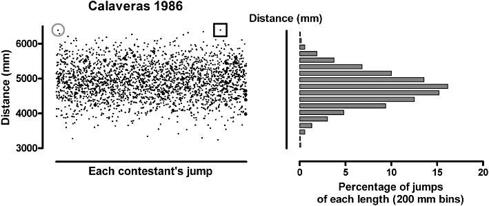
The distance jumped by each contestant is shown on the left. The square marks the record breaking jump of Rosie the Ribeter, and the circle is the runner-up, Jumping Jack Flash. On the right, the distribution of these distances is summarized.

The imaginary data come from a commonly encountered distribution and are summarized in a frequency curve (right side of Figure 1). This frequency function is ‘bell’-shaped, and is known as the Normal or Gaussian distribution. This distribution is a frequent pattern in biology, and can be described mathematically.

How effective is training frogs to jump? Would you bet on the result? Suppose you were able to take some frogs, at random, from these contestants, and train them to jump well. You would like to know if this training makes them do substantially better when they enter the competition. You might even want to place a bet on them, like Jim Smiley.

This is perhaps the most frequent question in biology that is subjected to statistical analysis: does a treatment make a difference? In fact, the standard test used is not posed in this way. You start with two groups of 20 frogs, both drawn at random from the competitors registered for the 1986 frog jumping competition: one group is left alone, you train the others, and then you see how far they all can jump. As we suggested in a previous article (Drummond and Vowler, 2011), we will display the results by plotting individual data, and calculate the mean distance jumped by each group (Figure 2). These sample mean values seem to be different and we suspect that the training could have had a positive effect. However, because the values in the 2500 frogs entered in the competition show quite a scatter, it is not likely that a small random sample will give us a mean that is quite the same as the mean of another random group.

Figure 2.

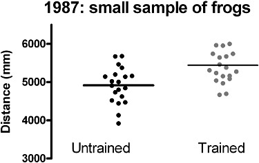
The effects of training a random sample of frogs. Is this effective?

We can examine whether there is indeed a training effect, by first assuming the opposite. That is, we assume that training has no effect on the mean distance jumped. If we propose that the mean values have been calculated from samples taken from the same population, any difference we do find between the mean values would be the consequence of chance alone. We calculate the probability (or P-value) of finding the observed difference between the mean distances jumped by the two groups, or something more extreme, given that they are taken from the same population. We compute this using a formula that relates the sizes of the differences between the values to the scatter of the values. This method of finding a shift in a set of variable's values is analogous to picking out a signal from background noise – which depends on the signal to noise ratio. We decide arbitrarily, but in common with many other researchers, that we will be willing to conclude that training has an effect if the probability of seeing this observed difference in the means, or a more extreme difference, is less than 5%, if truly the jumps came from the same population. The history of this concept and a more extensive explanation of the reasoning are detailed by Curran-Everett (Curran-Everett, 2009b).

Figure 3A shows the difference between the actual means we found, and also the range of differences between means that could occur, entirely by chance, on 95% of occasions. This is certainly not the only possible range; it is the range that we have deduced from observations of our sample. If we were to repeat the experiment with other similarly drawn samples, we would obtain similar but not identical sets of values, and derive similar but not identical sets of confidence intervals. The concept of confidence interval will be developed in subsequent articles: further details can be found elsewhere (Curran-Everett, 2009a).

Figure 3.

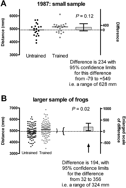
The effect of using a larger sample: the uncertainty of the estimate is less.

The calculated confidence interval extends from −79 to +549 mm, that is, a range of 628 mm. This range spans zero, which is consistent with the possibility that there is no difference between the means. Because our two groups have been randomly sampled from this population, we can calculate the probability that this difference in sample means (or a more extreme value) would have been found, if in fact the two population means were the same. This probability is 12%. We have to conclude, on the basis of the numbers that we have, and the arbitrary limit we have set ourselves, that there is insufficient evidence that training has changed the mean jumping distance. That does not mean that training frogs to jump further has no effect. It simply means that the results obtained remain consistent with the hypothesis that the two groups have been sampled from populations with the same mean values (Figure 1).

But … we did not take a very large sample. The larger the sample, the more precisely we can estimate the average length of the jumps in the sample we take, and thus any possible difference between the groups' jumping performance. So we go back and repeat our trial. This time we take the time and trouble to train 100 (randomly chosen) frogs to jump, and compare them with another 100 (randomly chosen) frogs that remain untrained. We now obtain a more precise estimate of the difference in means between the groups (Figure 3B). Using our new samples, we can calculate a new estimate of the difference. We estimate that the difference between the mean distance jumped is 194 mm. It is still an estimate of the true difference, which would only be found if we had even more time and resources to measure all the frogs. More importantly, we can also use the new larger samples to calculate a new confidence interval. We estimate the interval that would, with a probability of 95%, encompass that actual true difference (i.e. the benefit of training). Using the larger samples, the estimated 95% confidence interval is from 32 to 356 mm, a range of 324 mm. This confidence limit does not include zero, which is evidence against the null hypothesis. In addition, we use our new samples to calculate the probability that we would have obtained this difference in the means of the samples. We obtain a P-value of 2%. This suggests that our samples would have been unusual, if there were truly no difference in the means. Our larger sample has given us a more precise estimate of the difference in the means, and we could conclude that training improves the mean jumping performance. However, our estimate is that the mean improvement is only 194 mm, and a lot of untrained frogs can still jump further than some of the trained ones!

We found that the scatter of jump lengths made it hard to detect the effects of training when we used a small sample. We suspect that there could be a genetic factor behind the fact that frogs can jump different distances. We select the winner, Rosie, and the runner-up, Jumping Jack, and care for them over the winter. Next spring they produce a generation of tadpoles that become the only frogs to enter the 1988 competition. The year's results are shown in Figure 4 where we find a substantial improvement in performance, and also a reduction in the variation of the performances.

Figure 4.

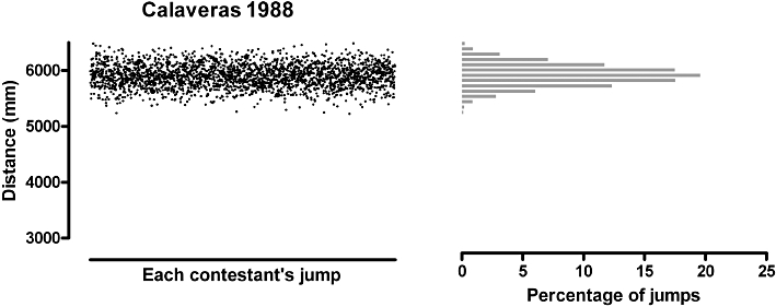
The performance of the offspring of Rosie and Jumping Jack: better than last year, and more consistent.

When we test the effects of training using these special frogs (Figure 5A), we now find a statistically significant result. In other words, if our null hypothesis were true, the probability is less than 5% that we could have obtained this result or something more extreme.

Figure 5.

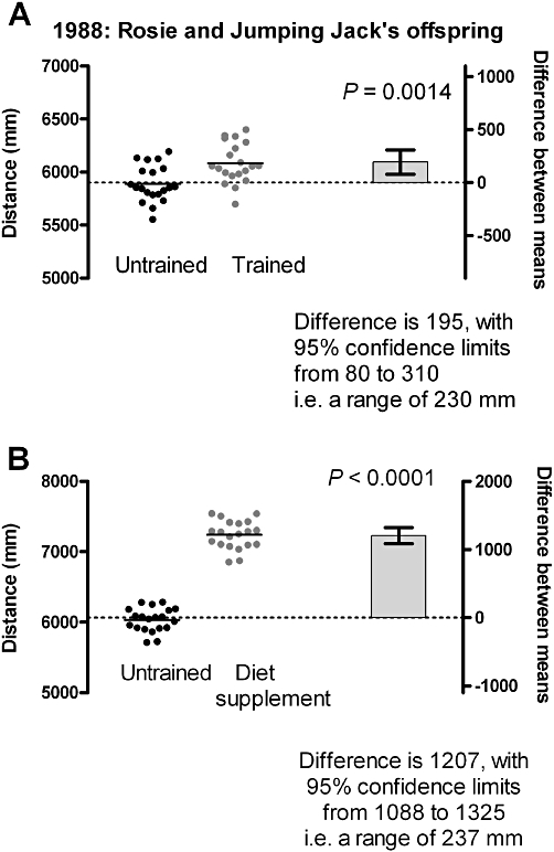
Two experiments on the offspring of Rosie and Jumping Jack: significant results with small numbers.

This result was significant, even though the effect is small and we only took small samples. Why should this be? With a genetically similar group of frogs, the ‘noise’ has become less and the effect is less concealed. However, as before, even though our data do not support the probability that the frogs are NOT affected by training, there is still a lot of scatter, and some bets on trained frogs are still going to lose! It looks like training is not going to give us a set of sure-fire winners, even though we have evidence that training has an effect.

Finally, we decide to try a dietary supplement on some more of Rosie's offspring (Figure 5B). Now we find there is a substantial improvement in the mean distance jumped, and the difference is not only large, but the probable range of differences is very small. Most people would consider these frogs certain winners!

It is clear that to be sure about these effects, we must be able to estimate the difference in means as precisely as possible. The difference may be large, which helps, or alternatively we can improve precision by taking a large sample, or by sampling from a population with reduced variation. In these latter cases, however, although we may have sufficient evidence to be convinced that there is a difference, the difference may not be large enough to be biologically important. This underlines yet again how simple statistical significance is difficult to interpret without an estimate of the effect size. What is often more relevant is an important size of the effect: in our example, the effect of the diet rather than the training.

We have ignored, in the last experiment, the fact that we have carried out several previous experiments. Each time we did an experiment, we accepted that there was a 5% chance of a false-positive result (i.e. we would conclude there was a difference, when in fact there was not one). This may increase the risk of concluding, purely by chance, that a difference exists when there actually is none: the more tests, the greater the risk that a false positive will occur. This, and strategies to tackle this possibility, will be addressed in a later article.

Conflicts of interest

None.

References

- Curran-Everett D. Explorations in statistics: confidence intervals. Adv Physiol Educ. 2009a;33:87–90. doi: 10.1152/advan.00006.2009. [DOI] [PubMed] [Google Scholar]
- Curran-Everett D. Explorations in statistics: hypothesis tests and P values. Adv Physiol Educ. 2009b;33:81–86. doi: 10.1152/advan.90218.2008. [DOI] [PubMed] [Google Scholar]
- Drummond GB, Vowler SL. Show the data, don't conceal them. Br J Pharmacol. 2011;163:208–210. doi: 10.1111/j.1476-5381.2011.01251.x. [DOI] [PMC free article] [PubMed] [Google Scholar]
- Twain M. The celebrated jumping frog of Calaveras County, and other sketches. In: Pritchett VS, editor. The Oxford Book of Short Stories. Oxford: Oxford University Press; 1867. pp. 61–66. [Google Scholar]