A Complete Solution for Dissecting Pure Main and Epistatic Effects of QTL in Triple Testcross Design

Abstract

Epistasis plays an important role in genetics, evolution and crop breeding. To detect the epistasis, triple test cross (TTC) design had been developed several decades ago. Classical procedures for the TTC design use only linear transformations Z₁, Z₂ and Z₃, calculated from the TTC family means of quantitative trait, to infer the nature of the collective additive, dominance and epistatic effects of all the genes. Although several quantitative trait loci (QTL) mapping approaches in the TTC design have been developed, these approaches do not provide a complete solution for dissecting pure main and epistatic effects. In this study, therefore, we developed a two-step approach to estimate all pure main and epistatic effects in the F₂-based TTC design under the F₂ and F_∞ metric models. In the first step, with Z₁ and Z₂ the augmented main and epistatic effects in the full genetic model that simultaneously considered all putative QTL on the whole genome were estimated using empirical Bayes approach, and with Z₃ three pure epistatic effects were obtained using two-dimensional genome scans. In the second step, the three pure epistatic effects obtained in the first step were integrated with the augmented epistatic and main effects for the further estimation of all other pure effects. A series of Monte Carlo simulation experiments has been carried out to confirm the proposed method. The results from simulation experiments show that: 1) the newly defined genetic parameters could be rightly identified with satisfactory statistical power and precision; 2) the F₂-based TTC design was superior to the F₂ and F_2:3 designs; 3) with Z₁ and Z₂ the statistical powers for the detection of augmented epistatic effects were substantively affected by the signs of pure epistatic effects; and 4) with Z₃ the estimation of pure epistatic effects required large sample size and family replication number. The extension of the proposed method in this study to other base populations was further discussed.

Introduction

Epistasis, the interaction between genes, plays an important role in genetics, evolution and crop breeding. First, it is an important genetic component in the genetic architecture of complex traits [1], [2]. Next, it can lead to heterosis [3]–[7], which is very important in hybrid breeding. In addition, it is a driving force in evolution and plays a central role in founder effect models of speciation [1], [8], [9]. Over the past several decades, many attempts have been made to detect the epistasis. One important attempt was triple test cross (TTC) design developed by Kearsey and Jinks [10], which is a powerful breeding design as well. Therefore, the great importance associated with the epistasis necessitates an in-depth study of the TTC design.

The TTC design is to cross the ith individual (i = 1,2,…n) of an F₂ population (or backcross, recombinant inbred lines (RIL) and near isogenic lines (NIL)) to the same three testers, the two inbred lines (P₁ and P₂) and their F₁, to produce 3n families. The design is considered the most efficient model as it provides not only a precise test for epistasis, but also unbiased estimates of additive and dominance components if epistasis is absent [10]. In early studies, only the phenotypic data of quantitative traits were used in the TTC to infer the nature of the additive, dominance and epistatic effects of polygenes using classical generation mean [11]–[13] and variance component analysis [10], [12], [14]–[17]. However, these conventional biometrical genetic procedures deal only with the collective effects of all the polygenes [6], [7], [11], [12]. The introduction of molecular markers has facilitated the mapping of quantitative trait loci (QTL) in numerous species, and substantial progress has been achieved in the detection of individual QTL and their interaction in the RIL- and NIL-based TTC designs.

In the RIL-based TTC designs, Kearsey et al. [12] employed the marker difference regression of Kearsey and Hyne [18] to detect QTL for 22 quantitative traits in Arabidopsis thaliana. Frascaroli et al. [16] used composite interval mapping [19] to identify main-effect QTL and the mixed linear model approach [20] to detect digenic epistatic QTL in the analyses of heterosis in maize. The method has been used to identify the main-effect QTL and digenic epistatic QTL underlying the heterosis of nine important agronomic and economic traits in rice by Li et al. [17]. However, the additive and dominant effects estimated from the above approaches are confounded with epistatic effect if epistasis is present. To overcome this issue, Melchinger et al. [21] derived quantitative genetic expectations of QTL main and interaction effects in the RIL-based TTC design. On their theoretical findings, using one-dimensional genome scans, we can estimate augmented additive and dominance effects [7] and QTL- by-genetic background interaction, whereas using two-way ANOVA between all pairs of marker loci, we can estimate additive-by-additive (aa) and dominance-by-dominance (dd) interactions. Kusterer et al. [22] applied the novel approaches of Melchinger et al. [7], [21] to detect QTL for heterosis of biomass-related traits in Arabidopsis. In the above studies, only one variable was involved at one time. To increase the power of QTL detection, Kusterer et al. [22] adopted multi-variable joint analysis [23], as proposed by Melchinger et al. [7] for QTL mapping in the NCIII design.

In the NIL-based TTC design, Melchinger et al. [21] used two QTL mapping methods to study heterosis in Arabidopsis. In the generation means approach, additive, dominance and QTL × genetic background epistasis effects were tested and estimated, and the approach along with particular two-segment NILs was applied by Reif et al. [24] to map aa digenic interaction. In addition, Zhu and Zhang [25] derived formulae for calculating the statistical power in the detection of epistasis; and Wang et al. [26] used interval mapping [27] to detect QTL underlying endosperm traits and demonstrated that the TTC provided a reasonably precise and accurate estimation of QTL positions and effects, especially the two dominant effects, which perfectly overcomes the drawback of the F_2:3 design.

In summary, two issues in the detection of QTL in the TTC need to be addressed. First, only a few studies are built on F₂-based TTC [25], [26], whereas most are built on RIL [7], [12], [16], [17], [21], [22] and NIL [6], [24]. Second, additive and dominance effects were confounded with QTL-by-genetic background interaction [7], [21], [22] and only aa and dd digenic interactions were evaluated in the RIL-based TTC [16], [17], [21], [22].

The objective of this study was to estimate, in an unambiguous and unbiased manner, all the main and epistatic effects of QTL in the F₂-based TTC design. A series of Monte Carlo simulation experiments was carried out to confirm the proposed approach. The extension of the new method to other base populations in the TTC was discussed as well.

Methods

Genetic design and data collection

An F₂ population was derived from two inbred lines (P₁ and P₂) that differed significantly in the quantitative traits of interest and possessed abundant polymorphism molecular markers. A random sample of n F₂ individuals (female parents) was backcrossed to three testers, the two parental lines and their F₁, to produce 3n families (, and ). All of the 3n families, each with m replications, were planted. Molecular marker information was observed from all of the n F₂ individuals, whereas quantitative traits were measured for all of the 3nm TTC progeny. The phenotypic observations were denoted by , where and 3 for , and ; and . The family means were denoted by 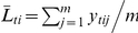. Following Kearsey and Jinks [10] and Melchinger et al. [21], we performed three linear transformations: , and . The association between and the marker genotypes of the F₂ plants were used to infer the genetic architecture of the trait.

Genetic models for mapping QTL in the F₂-based TTC design

The expected genetic values of , and depended on the choice of the metric. Two main metrics, the F₂ and F_∞ metrics, were adopted for the populations derived from the cross between the two inbred lines [28]-[30]. The derivation of the expected genetic values of , and under both the F₂ and the F_∞ metric models was presented in Table S1, Table S2, Table S3, Table S4, Table S5, Table S6, and Supporting Information S2. The genetic effect symbols adopted in this study were referred to Kao and Zeng [28].

Statistical genetic models for mapping QTL under the F₂ metric model

According to the expected genetic value of under the F₂ metric model in Table S5, the phenotypic value of can be described as:

(1)

where is the mean genotypic value of the F₂ population; and are additive and dominance effects of the kth QTL, respectively; , , and are additive-by-additive, additive-by-dominance, dominance-by-additive and dominance-by-dominance interactions between the 1st and 2nd QTL, respectively; , , , , and are dummy variables and determined by the genotype of the ith F₂ plant (Table S5); and is the residual error with an distribution. According to the results in Table S5, there are , and . To solve the genetic parameters, model (1) must be reduced to:

(2)

where , , 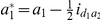, 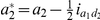and .

If the quantitative trait was controlled by QTL, model (2) should be extended to:

(3)

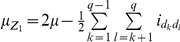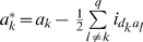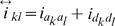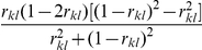
where model mean ; is augmented additive effect of QTL ; is augmented epistatic effect between QTL and ; and and are determined by the genotypes of the kth and lth QTL (marker) of the ith F₂ plant (Table 1). The coefficients for the genotype were integrated by the frequencies of and . The augmented epistatic effects () are ignored in Melchinger et al. [21], this may result in a bigger residual error and lower statistical power.

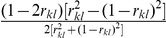
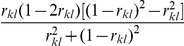
Table 1. Dummy variable values for genetic parameters in the genetic model of , and under various marker genotypes of F₂ plant and the F₂ and the F_∞ metric models.

Marker genotype of F2 plant	F2 metric model															F∞ metric model
	1	1	1	−1	−1		−r	−r	r	1	1	1	−1	−1	0	−r	−r	r
	1	0		−1	0	0	0	−r	0	1	0		−1	0		0	−r	0
	1	−1	0	−1	1		R	−r	−r	1	−1	0	−1	1	1	R	−r	−r
	0	1		0	−1	0	−r	0	0	0	1		0	−1		−r	0	0
	0	0		0	0		0	0		0	0		0	0		0	0
	0	−1		0	1	0	r	0	0	0	−1		0	1		R	0	0
	−1	1	0	1	−1		−r	R	−r	−1	1	0	1	−1	1	−r	R	−r
	−1	0		1	0	0	0	R	0	−1	0		1	0		0	R	0
	−1	−1	1	1	1		r	r	r	−1	−1	1	1	1	0	r	r	r

In the same way, the phenotypic value of can be described as:

(4)

where , , , and are determined by the genotype of the ith F₂ plant (Table S5); and is the residual error with an distribution. According to the results in Table S5, there are and . To solve the genetic parameters, model (4) must be reduced to:

(5)

where , , , and .

If the quantitative trait was controlled by QTL, model (5) should be extended to:

(6)

where model mean ; 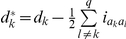is augmented dominance effect of QTL ; is augmented epistatic effect between QTL and ; and dummy variables and are determined by the genotypes of the kth and lth QTL of the ith F₂ plant (Table 1). The augmented epistatic effects () are overlooked in Melchinger et al. [21], this may result in a bigger residual error and lower statistical power.

Similarly, the phenotypic value of can be described as:

(7)

where ; is the recombination fraction between two QTL under study; and dummy variables , and are determined by the genotype of the ith F₂ plant (Table 1 and Table S5). Here pure ad, da and dd epistatic effects can be estimated with two-dimensional genome scans. This differs from that in Melchinger et al. [21], in which only dd epistasis is estimated with two-way ANOVA.

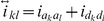
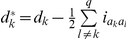
Models (3), (6) and (7) were working models for our QTL mapping approach in the F₂-based TTC design. Here we proposed a two-step approach to obtain all the pure main and epistatic effects in the presence of epistasis. In the first step, model (3) can be used to estimate the augmented additive () and epistatic () effects, model (6) can be used to estimate the augmented dominance () and epistatic () effects, and model (7) can be used to estimate three types of pure epistatic effects (, and ). In the second step, all estimated epistatic effects in models (3), (6) and (7) were integrated for the estimation of all four types of the pure epistatic effects using 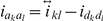, and . These pure epistatic effects further integrate with the estimates of both and for the estimation of pure additive and dominance effects, using and . When epistasis is absent, pure additive () and dominance () effects can be directly obtained from model (3) and model (6), respectively.

Genetic models for mapping QTL under the F_∞ metric model

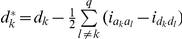
With , and genetic models for mapping QTL under the F_∞ metric model have the same forms as described in models (3), (6) and (7), respectively. The detailed derivation was described in Table S6 and Supporting information S1 and the detailed comparisons were given in Tables 1 and 2. The pure epistatic effects under the two metrics are calculated in the same way and the pure additive and dominance effects under the two metrics are calculated in different ways, here and .

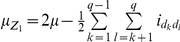
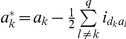
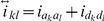
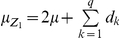
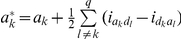
Table 2. Genetic parameter component and parameter estimation method for the genetic models of Z₁, Z₂ and Z₃ under the F₂ and the F_∞ metric models.

Data	Model	Model parameter components						Parameter estimation method
		F2 metric model			F∞ metric model
		Model mean	Augmented main effect	Augmented epistatic effect	Model mean	Augmented main effect	Augmented epistatic effect
Z1	(3)							Empirical Bayes
Z2	(6)							Empirical Bayes
Z3	(7)		—			—		Maximum likelihood

Genetic parameter estimation

Models (3) and (6) have a uniform appearance. However, the true number of QTL () is hard to determine. Variable selection via a stepwise regression or a stochastic search variable selection is the common procedure for epistatic QTL analysis. But these methods are computationally intensive and may not be optimal [31]–[33]. Thus, we adopted the empirical Bayes (E-Bayes) method of Xu [33] for the estimation of parameters in the above models. The E-Bayes approach assumes that there is one QTL standing on each marker throughout the genome and shrinks the genetic effects of all “nonsignificant” QTL toward zero. Here, we only gave some necessary procedures; for the technical details of the E-Bayes refer to the original study of Xu [33].

Models (3) and (6) can be uniformly written as:

(8)

where is the model mean; is the augmented main effect of the kth QTL; is the augmented epistatic effect between the kth and lth QTL; is the total number of genetic effects, including the augmented main and epistatic effects; and is the residual error. Model (8) can be expressed in matrix form:

(9)

where ; ; ; ; 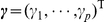and .

In the expectation and maximization (EM) algorithm of the E-Bayes method [33], model (9) is a typical mixed model and is treated as a fixed effect, whereas is treated as a random effect. Therefore, has a multivariate normal distribution with the mean and the variance-covariance matrix .

In the EM algorithm of E-Bayes, the genetic parameters are the focus of interest and the normal prior is assigned to , i.e., and is further assigned a scaled inverse prior, i.e., . The has uniform prior distribution.

The EM algorithm procedures are as follows:

1) Choose and assign initial values: , , .

2) E-step: the best linear unbiased prediction (BLUP) estimation of the expectation of the quadratic term

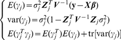(10)

3) M-step: the maximum-likelihood estimation for , fixed effects and residual variance

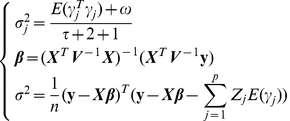(11)

4) repeat steps 2) - 3) until a certain criterion of convergence is satisfied, e.g. the difference of parameter estimate values between two adjacent iterations were less than 10⁻¹⁰.

In addition, we performed a two-dimension scan using the maximum likelihood approach for the estimation parameters in models (7).

Likelihood ratio test

If we only want to report QTL with relatively large effects and give readers accurate information about how significant the identified QTL were, statistical test should be conducted. The usual likelihood ratio test (LRT) cannot be carried out with the E-Bayes method owing to an oversaturated epistatic genetic model. We proposed the following two-stage selection process to screen the QTL [31]. In the first stage, all QTL with 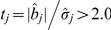are picked up. In the second stage, the epistatic genetic model is modified so that only effects past the first round of selection are included in the model. Owing to the smaller dimensionality of the reduced model, we can use the maximum likelihood method to re-analyze the data and perform the LRT [31]. The test statistic is

(12)

where is the parameters vector in the statistical genetic model in the second stage analysis of model (8); is the parameters vector in excluding the currently tested genetic effect ; and are the log maximum likelihood function for and , respectively. For simplicity, we took and 3.0 as the critical values in our small and larger genome simulation experiments, respectively.

Results

Experiment I

The purpose of the simulation experiment was: (1) to evaluate the statistical performance of the proposed approach; (2) to compare the proposed method with previous approaches, such as Kearsey et al. [12], Frascaroli et al. [16] and Li et al. [17] or Melchinger et al. [7], [21] and Kusterer et al. [22], according to statistical power, standard deviation and accuracy measure; and (3) to compare the TTC design with the F₂ and F_2:3 genetic designs.

The simulated genome consisted of three chromosomes (chr1, chr2 and chr3), and 11 evenly spaced markers covered each chromosome with an average marker interval of 10.0 cM. We simulated three main-effect QTL and one pair-wise interaction QTL, all of which overlapped with markers. All three main-effect QTL were located at the center (50.0 cM) of each chromosome, and QTL₂ on chr2 interacted with QTL₃ on chr3. The genetic parameters under both the F₂ and the F_∞ metric models were as follows: ; and for QTL₁; and for QTL₂; and for QTL₃; , , and for the epistatic effects between QTL₂ and QTL₃. The marginal heritabilities of these genetic effects varied from 1.01% to 36.54%. The sample size (n), the number of individual in the F₂ population, was set at two levels: 200 and 400. The number of individuals (m) for each TTC family was set at 1, 5 and 10. The environmental variance () was set at 4.00 and 1.00. To implement the last objective of the simulation experiment, two other kinds of populations, the F₂ and F_2:3 populations, were also simulated. However, molecular marker information for all three populations was derived from the corresponding F₂ individuals. Each treatment was replicated 200 times for the TTC and F_2:3 designs and 400 times for the F₂ design. In the analyses of the TTC family data, two approaches were adopted: 1) Method A, the proposed method in this study, and 2) Method B, the modified method of Kearsey et al. [12], Frascaroli et al. [16] and Li et al. [17] or Melchinger et al. [7], [21] and Kusterer et al. [22], by removing the augmented epistatic effects from models (3) and (6). In the analyses of the F₂ and F_2:3 datasets, all of the main effects and all of the pair-wise interaction effects for all of the markers on the whole genome were simultaneously included in the genetic model. For each simulated QTL, we counted the samples in which the LOD statistic was greater than 2.5 and the identified QTL was within 20.0 cM of the simulated QTL. The estimate for QTL parameter was the average of the corresponding estimates in the counted samples. The ratio of the number of such samples to the total number of replicates represented the empirical power of this QTL.

To achieve the first objective of the simulation experiment, , and were analyzed by Method A. In the first step, with or 33 augmented additive or dominance effects ( or ) and 528 augmented epistatic effects ( or ) were estimated, and with 1584 pure epistatic effects (, and ) were estimated. All the effects were tested by likelihood ratio statistic in order that real QTL could be identified. The results for detected QTL under the F₂ metric model were listed in Table 3, Table 4, Table 5. The results show that the newly defined parameters, i.e., , , (), and , were estimated in an almost unambiguous and unbiased manner, and all of the main-effect QTL were identified with a high statistical power and precision in the estimated effects and positions of the QTL by taking the TTC family mean as the unit of phenotypic measurement. The augmented epistatic QTL ( and ) were also well detected, except for the situation when , and . In the second step, all the pure main and epistatic effects would be estimated in an unbiased manner (Table 6). It should also be noted that a large sample (), a greater family replication number (), and moderate QTL heritability () are needed for the partition of the augmented epistatic effects ( and ) into its components (, , and ), and detecting epistasis is more difficult than detecting epistasis (Tables 5 and 6). The theoretical explanation is that (also ) has a larger contribution to the genetic variance of than ( when , Supporting Information S2). In addition, the powers in the detection of the augmented epistatic effects ( in Table 3 and in Table 4) were always much higher than those of pure epistatic effects (, and in Table 5). The possible explanations lie in that 1) the augmented epistatic effects ( and ) were the sum of two epistatic effects with the same signs in Experiment I and were inflated, and 2) these epistatic effects have different contributions to the genetic variances of , and (Supporting Information S2).

Table 3. Comparison of the proposed approach (Method A) with previous method (Method B) that does not consider augmented epistasis for mapping QTL of Z ₁ under the F₂ metric model.

			Method A**															Method B
n	m		MSe		QTL1			QTL2			QTL3			QTL2×QTL3				MSe		QTL1			QTL2			QTL3
					a1 *	Position	Power	a2 *	Position	Power	a3 *	Position	Power		Position2	Position3	Power			a1	Position	Power	a2	Position	Power	a3	Position	Power
Parameter values				199.25	1.50	50.00		1.50	50.00		-1.75	50.00		2.50	50.00	50.00				1.50	50.00		2.00	50.00		-1.00	50.00
200	1	4.00	13.321(1.370)	200.438(0.514)	1.641(0.246)	50.135(8.410)	0.740	1.625(0.290)	49.937(7.779)	0.790	-1.808(0.312)	50.160(7.069)	0.935	4.218(0.539)	40.000(8.165)	52.500(12.583)	0.020	13.363(1.357)	200.502(0.258)	1.648(0.251)	50.068(7.781)	0.740	1.631(0.286)	50.127(7.249)	0.785	-1.827(0.304)	50.437(7.018)	0.915
		1.00	7.013(0.727)	200.387(0.477)	1.508(0.241)	49.682(4.104)	0.980	1.511(0.249)	50.459(4.332)	0.980	-1.779(0.258)	50.103(3.311)	1.000	3.143(0.400)	47.692(8.321)	51.538(6.887)	0.065	7.053(0.695)	200.503(0.199)	1.510(0.240)	49.887(3.857)	0.980	1.511(0.252)	50.606(4.899)	0.990	-1.779(0.259)	50.047(3.670)	1.000
	5	4.00	2.643(0.335)	199.638(0.681)	1.485(0.161)	50.061(0.725)	0.990	1.505(0.166)	49.950(0.707)	1.000	-1.733(0.154)	50.048(0.478)	1.000	2.689(0.378)	50.112(3.482)	49.346(4.197)	0.630	2.933(0.305)	200.495(0.118)	1.500(0.163)	50.010(1.017)	0.990	1.517(0.182)	50.027(0.382)	0.995	-1.736(0.170)	50.045(0.454)	1.000
		1.00	1.351(0.145)	199.261(0.151)	1.498(0.111)	50.011(0.156)	1.000	1.479(0.126)	49.991(0.573)	1.000	-1.744(0.109)	49.985(0.217)	1.000	2.499(0.243)	50.201(2.000)	49.749(1.863)	0.995	1.732(0.165)	200.509(0.100)	1.489(0.135)	49.932(0.752)	1.000	1.485(0.151)	49.994(0.546)	1.000	-1.738(0.130)	49.986(0.282)	1.000
	10	4.00	1.270(0.138)	199.268(0.219)	1.505(0.118)	50.000(0.000)	1.000	1.492(0.116)	50.000(0.000)	1.000	-1.746(0.097)	49.998(0.235)	1.000	2.494(0.279)	49.795(2.479)	50.051(1.899)	0.975	1.651(0.159)	200.506(0.090)	1.504(0.133)	49.984(0.353)	1.000	1.487(0.159)	50.000(0.000)	1.000	-1.750(0.129)	49.984(0.350)	1.000
		1.00	0.679(0.076)	199.247(0.115)	1.496(0.078)	50.007(0.099)	1.000	1.494(0.082)	50.011(0.160)	1.000	-1.752(0.073)	50.018(0.195)	1.000	2.515(0.170)	50.000(0.000)	49.934(0.740)	0.990	1.067(0.098)	200.506(0.073)	1.502(0.104)	50.011(0.438)	1.000	1.502(0.132)	50.008(0.112)	1.000	-1.742(0.114)	50.021(0.299)	1.000
400	1	4.00	13.101(1.008)	200.250(0.639)	1.522(0.233)	50.202(4.828)	0.990	1.534(0.242)	49.462(2.959)	0.995	-1.755(0.246)	50.000(3.023)	0.990	3.241(0.333)	50.000(5.872)	49.667(4.901)	0.150	13.207(1.003)	200.488(0.187)	1.522(0.236)	49.898(3.911)	0.985	1.530(0.243)	49.463(2.959)	1.000	-1.760(0.245)	49.950(2.930)	0.995
		1.00	6.797(0.485)	199.647(0.667)	1.502(0.176)	50.000(1.743)	0.990	1.475(0.181)	50.017(1.439)	1.000	-1.726(0.185)	50.098(1.001)	0.995	2.650(0.302)	50.156(5.468)	49.688(4.514)	0.640	7.082(0.442)	200.504(0.131)	1.501(0.184)	50.101(1.740)	0.990	1.479(0.180)	50.108(1.369)	0.990	-1.733(0.194)	50.078(0.776)	0.990
	5	4.00	2.544(0.185)	199.255(0.210)	1.515(0.125)	50.014(0.192)	1.000	1.498(0.098)	49.997(0.301)	1.000	-1.745(0.120)	49.989(0.330)	1.000	2.483(0.283)	50.136(2.150)	50.035(1.612)	0.985	2.924(0.209)	200.500(0.082)	1.517(0.130)	50.020(0.281)	1.000	1.498(0.110)	50.029(0.526)	1.000	-1.746(0.136)	49.996(0.405)	1.000
		1.00	1.349(0.102)	199.246(0.110)	1.499(0.076)	50.007(0.242)	1.000	1.509(0.068)	50.000(0.000)	1.000	-1.761(0.073)	50.000(0.000)	1.000	2.495(0.162)	49.987(0.180)	49.994(0.090)	1.000	1.733(0.106)	200.503(0.063)	1.502(0.090)	50.003(0.284)	1.000	1.509(0.091)	50.014(0.202)	1.000	-1.757(0.095)	50.000(0.000)	1.000
	10	4.00	1.281(0.087)	199.240(0.139)	1.504(0.077)	50.000(0.000)	1.000	1.503(0.078)	49.993(0.168)	1.000	-1.750(0.078)	50.012(0.123)	1.000	2.506(0.204)	50.000(0.000)	49.938(0.617)	1.000	1.674(0.111)	200.498(0.065)	1.501(0.090)	50.000(0.000)	1.000	1.494(0.098)	50.000(0.000)	1.000	-1.749(0.104)	50.013(0.127)	1.000
		1.00	0.677(0.055)	199.250(0.081)	1.501(0.052)	50.000(0.000)	1.000	1.493(0.054)	50.000(0.000)	1.000	-1.754(0.053)	49.994(0.079)	1.000	2.505(0.118)	49.991(0.126)	50.009(0.126)	1.000	1.064(0.067)	200.505(0.053)	1.500(0.068)	50.000(0.000)	1.000	1.495(0.082)	50.004(0.062)	1.000	-1.758(0.088)	49.994(0.089)	1.000

* n denotes sample size; m is number of replications; and is residual variance for the phenotypic trait value . The numbers in parentheses are standard deviation and the same is true for the later tables except for Table 6 to Table 8.

** , , , and , see model (3) for details.

Table 4. Comparison of the proposed approach (Method A) with previous method (Method B) that does not consider augmented epistasis for mapping QTL of Z ₂ under the F₂ metric model.

			Method A**															Method B
n	m		MSe		QTL1			QTL2			QTL3			QTL2×QTL3				MSe		QTL1			QTL2			QTL3
					d 1 *	Position	Power	d 2 *	Position	Power	d 3 *	Position	Power		Position2	Position3	Power			d 1	Position	Power	d 2	Position	Power	d 3	Position	Power
Parameter values				2.50	1.50	50.00		-1.50	50.00		1.50	50.00		2.50	50.00	50.00				1.50	50.00		-1.00	50.00		2.00	50.00
200	1	4.00	13.033(1.479)	2.566(0.351)	1.658(0.275)	49.351(6.635)	0.770	-1.631(0.275)	49.379(8.184)	0.725	1.617(0.284)	49.737(8.608)	0.760	4.019(0.506)	51.429(10.885)	45.143(14.219)	0.175	13.297(1.424)	2.525(0.252)	1.661(0.292)	49.545(5.906)	0.785	-1.636(0.282)	49.801(7.346)	0.755	1.632(0.292)	49.400(7.877)	0.750
		1.00	6.834(0.761)	2.513(0.227)	1.518(0.237)	50.127(4.821)	0.960	-1.511(0.240)	49.848(4.342)	0.985	1.518(0.235)	50.084(5.822)	0.990	3.002(0.447)	53.133(11.469)	49.157(10.146)	0.415	7.116(0.741)	2.509(0.192)	1.516(0.237)	50.052(4.007)	0.970	-1.520(0.237)	49.846(4.245)	0.975	1.529(0.223)	49.949(5.392)	0.985
	5	4.00	2.525(0.276)	2.485(0.117)	1.516(0.155)	50.003(0.836)	1.000	-1.496(0.166)	49.942(1.187)	1.000	1.494(0.166)	49.899(1.000)	0.995	2.537(0.416)	50.011(5.056)	50.320(5.746)	0.905	2.906(0.299)	2.479(0.121)	1.527(0.157)	49.982(1.385)	1.000	-1.495(0.184)	49.899(0.926)	0.995	1.512(0.177)	49.997(0.036)	0.995
		1.00	1.338(0.146)	2.502(0.096)	1.486(0.114)	49.926(0.533)	1.000	-1.490(0.098)	49.978(0.313)	1.000	1.507(0.108)	50.033(0.308)	1.000	2.489(0.260)	49.571(2.067)	50.236(2.416)	1.000	1.721(0.163)	2.503(0.087)	1.482(0.137)	49.926(0.956)	0.995	-1.488(0.130)	50.031(0.661)	0.995	1.515(0.135)	50.044(0.629)	0.995
	10	4.00	1.269(0.132)	2.512(0.109)	1.497(0.104)	50.022(0.306)	1.000	-1.507(0.126)	50.004(0.311)	1.000	1.497(0.109)	50.010(0.451)	1.000	2.530(0.319)	50.045(2.162)	50.239(2.571)	1.000	1.673(0.150)	2.510(0.093)	1.498(0.122)	50.018(0.261)	1.000	-1.518(0.147)	50.021(0.299)	1.000	1.495(0.128)	50.028(0.490)	0.995
		1.00	0.686(0.075)	2.502(0.070)	1.496(0.079)	50.000(0.000)	1.000	-1.498(0.075)	49.993(0.098)	1.000	1.506(0.073)	49.994(0.092)	1.000	2.490(0.186)	49.967(0.471)	50.017(0.238)	0.995	1.073(0.096)	2.501(0.071)	1.502(0.096)	50.000(0.000)	1.000	-1.495(0.122)	50.041(0.480)	1.000	1.515(0.118)	50.000(0.000)	1.000
400	1	4.00	12.764(1.022)	2.473(0.245)	1.523(0.238)	50.282(3.733)	0.990	-1.487(0.237)	50.063(4.238)	0.995	1.504(0.239)	49.594(4.020)	0.985	2.995(0.478)	50.938(8.835)	49.792(9.059)	0.480	13.128(0.980)	2.486(0.186)	1.515(0.251)	50.355(3.867)	0.995	-1.503(0.225)	49.899(4.505)	0.990	1.519(0.239)	49.848(4.331)	0.990
		1.00	6.807(0.523)	2.510(0.143)	1.498(0.174)	50.127(1.460)	0.990	-1.475(0.185)	50.394(2.379)	0.995	1.478(0.171)	49.952(1.959)	1.000	2.574(0.376)	49.586(6.110)	50.296(6.585)	0.845	7.179(0.498)	2.506(0.137)	1.497(0.170)	50.115(1.763)	0.995	-1.471(0.188)	50.151(1.582)	0.995	1.480(0.183)	49.789(1.730)	1.000
	5	4.00	2.544(0.195)	2.510(0.097)	1.498(0.116)	49.981(0.203)	1.000	-1.499(0.111)	50.000(0.000)	1.000	1.494(0.124)	50.020(0.390)	1.000	2.472(0.309)	49.897(2.057)	50.398(3.529)	0.990	2.933(0.212)	2.508(0.080)	1.495(0.133)	49.984(0.163)	1.000	-1.500(0.131)	49.994(0.301)	1.000	1.490(0.143)	50.000(0.000)	1.000
		1.00	1.348(0.101)	2.500(0.075)	1.502(0.081)	49.991(0.262)	1.000	-1.511(0.076)	50.009(0.131)	1.000	1.497(0.077)	50.016(0.165)	1.000	2.507(0.178)	50.017(0.235)	49.983(0.235)	1.000	1.736(0.110)	2.500(0.065)	1.502(0.100)	49.985(0.216)	1.000	-1.510(0.103)	49.991(0.130)	1.000	1.497(0.096)	50.000(0.000)	1.000
	10	4.00	1.261(0.089)	2.504(0.071)	1.500(0.079)	50.029(0.240)	1.000	-1.503(0.076)	49.996(0.058)	1.000	1.499(0.074)	50.000(0.000)	1.000	2.489(0.208)	50.022(0.249)	49.967(0.326)	1.000	1.650(0.117)	2.506(0.071)	1.498(0.093)	50.028(0.236)	1.000	-1.510(0.099)	50.000(0.258)	1.000	1.501(0.098)	50.002(0.215)	1.000
		1.00	0.677(0.054)	2.496(0.065)	1.504(0.058)	50.007(0.092)	1.000	-1.491(0.056)	50.000(0.000)	1.000	1.502(0.054)	49.993(0.068)	1.000	2.512(0.128)	50.012(0.163)	49.994(0.082)	1.000	1.069(0.074)	2.498(0.051)	1.502(0.068)	49.998(0.167)	1.000	-1.490(0.083)	49.996(0.166)	1.000	1.500(0.087)	49.996(0.054)	1.000

* n denotes sample size; m is number of replications; and is residual variance for the phenotypic trait value .

** , , , and , see Model (6) for details.

Table 5. Mapping QTL for Z ₃ under the F₂ metric model.

n	m		MSe		QTL2×QTL3
						Power		Power		Power	Position2	Position3
Parameter values				0.50	1.50		1.00		1.50		50.00	50.00
200	1	4.00	49.410(4.534)	0.508(0.515)	4.283(0.377)	0.045	5.353(0.376)	0.010	6.659(1.376)	0.025	50.250(8.293)	49.450(7.843)
		1.00	32.103(3.311)	0.535(0.396)	3.716(0.235)	0.060	4.208(0.840)	0.015	4.751(0.281)	0.010	50.050(8.175)	50.600(7.274)
	5	4.00	9.993(0.981)	0.498(0.218)	2.499(0.254)	0.155	2.302(0.300)	0.030	3.471(0.421)	0.045	49.750(7.120)	50.050(6.458)
		1.00	6.367(0.609)	0.514(0.175)	2.054(0.244)	0.320	1.932(0.233)	0.120	2.698(0.324)	0.110	49.900(6.260)	50.350(5.050)
	10	4.00	4.961(0.502)	0.509(0.158)	1.809(0.253)	0.440	1.748(0.222)	0.135	2.336(0.300)	0.150	49.950(5.888)	49.850(4.424)
		1.00	3.158(0.338)	0.505(0.120)	1.627(0.252)	0.815	1.392(0.178)	0.310	2.088(0.306)	0.370	49.650(4.179)	50.150(3.396)
400	1	4.00	50.246(3.427)	0.489(0.350)	3.511(0.393)	0.080	3.556(0.184)	0.020	5.020(0.519)	0.050	49.800(7.432)	50.100(7.434)
		1.00	31.734(2.121)	0.511(0.271)	2.838(0.406)	0.150	2.778(0.332)	0.045	4.008(0.685)	0.040	50.250(7.328)	49.550(6.821)
	5	4.00	10.052(0.675)	0.500(0.152)	1.903(0.253)	0.460	1.739(0.182)	0.135	2.534(0.267)	0.165	50.900(5.947)	50.250(4.853)
		1.00	6.391(0.489)	0.515(0.123)	1.627(0.260)	0.800	1.450(0.191)	0.225	2.009(0.289)	0.350	49.850(4.646)	50.300(3.739)
	10	4.00	5.003(0.386)	0.506(0.124)	1.540(0.277)	0.915	1.319(0.190)	0.375	1.882(0.256)	0.490	50.100(3.750)	50.300(2.820)
		1.00	3.174(0.222)	0.495(0.081)	1.495(0.246)	0.995	1.117(0.179)	0.755	1.633(0.263)	0.820	50.400(2.981)	50.250(1.859)

* n denotes sample size; m is family replication number; and is residual variance for the phenotypic trait value .

, see Model (7) for details.

Table 6. Estimation of pure main and epistatic effects of QTL in the F₂-based TTC design using the two-step approach under the cases of n = 400, m = 10 and (200 replicates).

Metric	Statistics	QTL1		QTL2		QTL3		QTL2×QTL3
		a 1	d 1	a 2	d 2	a 3	d 3
Parameter values		1.50	1.50	2.00	-1.00	-1.00	2.00	1.00	1.50	1.00	1.50
F2	Mean	1.501	1.504	2.028	-1.128	-1.025	1.865	0.886	1.466	1.075	1.633
	SD	0.052	0.058	0.108	0.214	0.100	0.214	0.262	0.200	0.190	0.263
	Power	1.000	1.000	1.000	1.000	1.000	1.000	0.820	0.995	0.995	0.820
F∞	Mean	1.502	1.504	2.049	-1.051	-1.062	1.940	0.797	1.468	1.080	1.724
	SD	0.055	0.063	0.213	0.305	0.193	0.306	0.263	0.224	0.219	0.264
	Power	1.000	1.000	1.000	1.000	1.000	1.000	0.670	0.990	0.990	0.670

To achieve the second objective of the simulation experiment, and were re-analyzed by method B and the results under the F₂ metric model were also listed in Tables 3 and 4. The results show that the Z ₁ and Z ₂ could still be used to unbiasedly estimate QTL additive () and dominance effect () when the QTL (QTL₁) acted independently; but provided biased estimation of QTL additive ( and ) and dominance effects ( and ) when the QTL acted dependently (QTL₂ and QTL₃). The additive ( and ) and dominance effects ( and ) of interactive QTL obtained by Method B in Tables 3 and 4 were indeed the newly defined additive effects ( and ) and the new dominance effects ( and ) with slightly poorer precision (little larger in standard deviation) in estimated QTL effects and positions and lower statistical power. This means that the new method was better than the previous methods of Kearsey et al. [12], Frascaroli et al. [16] and Li et al. [17] in the presence of epistasis. The higher statistical power and smaller error variance for method A over method B shows that the new method was also superior to the methods of Melchinger et al. [7], [21] and Kusterer et al. [22].

To achieve the third objective of the simulation experiment, the F₂ and F_2:3 data were analyzed and the results under the F₂ metric model were listed in Tables 7 and 8. The results show that many effects could be estimated in an unambiguous and unbiased manner in the F₂ and F_2:3 genetic designs. In the situation of , the F₂ design was superior to the both TTC and F_2:3 designs. The reasons are as follows. In all the above three designs, marker genotypes were from F₂ individuals. If , genotype sampling error was large for both TTC and F_2:3 designs. Meanwhile, the proposed approach in this study did not consider the mixed distribution of the F_2:3 (or TTC) progeny derived from heterozygous F₂ parents. However, the powers in the detection of the main and epistatic QTL were smaller for the F₂ design than for the TTC design with (or 10) when sample size () was small and/or environmental variance () was large, and the same trend was obtained for the precision of the estimates for the effects and the positions of the main and epistatic QTL. For example, when and , the power for main effects and were 0.850 and 0.775 and the standard deviation (SD) were 0.253 and 0.308, respectively, in F₂ design (Table 7); while the power for and were 1.000 and 1.000 and the SD were 0.118 and 0.104, respectively, in TTC design with a family replication of 10 (Tables 3 and 4). This may be due to the fact that the phenotypic value is measured from F₂ individuals and from the TTC family, and the family mean can be used to decrease the residual variance and to improve the precision of the phenotypic data. Both the TTC and F_2:3 designs use family mean to decrease environmental variance and improve the precision of phenotype of quantitative trait. In addition, the dominant components decrease significantly in the F_2:3 design due to its self-crossing, and the statistical powers for detecting dominance effects, additive by dominance (dominance by additive) epistatic effect and especially dominance by dominance epistatic effect in the F_2:3 design will be lower than that in the TTC design. 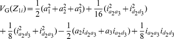For example, when , and , the power of 0.170 for in F_2:3 (Table 8) was much lower than that of 0.490 in the TTC (Table 5). The genetic variance contributed by the simulated three QTL under TTC and F_2:3 designs were (Supporting Information S2):

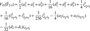Table 7. Results of QTL mapping in F₂ population under the F₂ metric model (400 replications).

n		Statistics	MSe		QTL1			QTL2			QTL3			QTL2×QTL3
					a1	d1	Position	a2	d2	Position	a3	d3	Position					Position2	Position3
Parameter values				100.00	1.50	1.50	50.00	2.00	-1.00	50.00	-1.00	2.00	50.00	1.00	1.50	1.00	1.50	50.00	50.00
200	4.00	Mean	4.016	100.051	1.480	1.571	50.193	1.920	-1.267	49.951	-1.036	1.940	50.138	1.320	1.813	1.637	2.317	50.413	50.233
		SD	0.613	0.336	0.253	0.308	2.522	0.307	0.220	2.059	0.197	0.357	3.825	0.225	0.335	0.255	0.370	9.245	8.089
		Power			0.850	0.775		0.963	0.313		0.488	0.935		0.418	0.540	0.158	0.200
	1.00	Mean	0.979	99.984	1.469	1.479	50.013	1.979	-0.971	50.077	-0.961	1.967	49.962	0.980	1.485	1.032	1.516	50.086	50.058
		SD	0.137	0.142	0.133	0.179	0.271	0.132	0.160	0.867	0.141	0.184	1.649	0.178	0.272	0.193	0.311	2.974	2.940
		Power			0.998	0.993		1.000	0.920		0.923	0.998		0.960	0.995	0.730	0.848
400	4.00	Mean	3.952	99.963	1.465	1.495	49.922	1.974	-1.039	49.920	-0.984	2.001	49.894	1.058	1.548	1.258	1.768	50.180	50.311
		SD	0.340	0.207	0.202	0.211	1.130	0.191	0.184	1.757	0.156	0.231	2.018	0.226	0.313	0.238	0.304	5.795	4.453
		Power			0.973	0.963		1.000	0.740		0.808	1.000		0.783	0.893	0.425	0.525
	1.00	Mean	0.970	99.995	1.498	1.504	49.998	1.997	-0.987	49.999	-0.994	2.000	50.005	0.995	1.502	0.997	1.531	49.959	49.952
		SD	0.079	0.065	0.078	0.111	0.080	0.085	0.111	0.090	0.089	0.111	0.369	0.119	0.166	0.163	0.237	0.966	1.364
		Power			1.000	1.000		1.000	0.993		0.998	1.000		0.995	1.000	0.985	0.998

* n denotes sample size; and is residual variance for the phenotypic trait value .

Table 8. Results of QTL mapping in F_2:3 population under the F₂ metric model (200 replications).

n	m		Statistics	MSe		QTL1			QTL2			QTL3			QTL2×QTL3
						a 1	d 1	Position	a 2	d 2	Position	a 3	d 3	Position					Position2	Position3
Parameter values					100.00	1.50	1.50	50.00	2.00	-1.00	50.00	-1.00	2.00	50.00	1.00	1.50	1.00	1.50	50.00	50.00
200	1	4.00	Mean	7.447	99.577	1.555	3.266	49.298	1.644	-2.965	50.408	-1.432	3.056	48.289	1.568	3.661	3.724	6.774	49.180	49.727
			SD	0.992	0.442	0.350	0.363	6.508	0.303	0.182	5.546	0.256	0.396	9.174	0.279	.	0.756	0.673	15.060	11.073
			Power			0.260	0.035		0.485	0.015		0.160	0.040		0.130	0.005	0.190	0.010
		1.00	Mean	4.598	99.659	1.520	2.492	49.739	1.629	-2.321	50.556	-1.316	2.495	49.191	1.213	2.676	3.005	5.471	48.164	50.340
			SD	0.625	0.417	0.276	0.431	5.123	0.303	0.251	4.390	0.218	0.383	5.834	0.191	0.247	0.570	0.689	16.695	10.972
			Power			0.535	0.095		0.720	0.015		0.260	0.095		0.320	0.015	0.260	0.015
	5	4.00	Mean	1.647	99.756	1.451	1.875	49.996	1.688	-1.675	50.053	-1.205	1.874	49.470	0.986	2.023	2.139	3.924	50.490	49.984
			SD	0.228	0.327	0.205	0.450	1.910	0.284	0.303	3.002	0.216	0.352	4.288	0.171	0.413	0.520	1.001	7.294	7.627
			Power			0.810	0.150		0.950	0.165		0.630	0.350		0.785	0.155	0.265	0.030
		1.00	Mean	0.958	99.825	1.449	1.601	49.905	1.780	-1.464	49.805	-1.132	1.743	49.969	0.973	1.666	1.684	3.168	49.669	50.851
			SD	0.156	0.344	0.170	0.314	1.741	0.258	0.302	2.049	0.222	0.387	3.680	0.142	0.307	0.409	0.453	4.729	5.057
			Power			0.965	0.405		0.965	0.375		0.780	0.570		0.975	0.415	0.255	0.105
	10	4.00	Mean	0.798	99.912	1.486	1.562	50.019	1.808	-1.411	50.094	-1.119	1.661	50.083	0.970	1.602	1.542	2.957	49.405	49.872
			SD	0.122	0.282	0.113	0.259	0.946	0.245	0.241	1.606	0.188	0.316	2.209	0.157	0.305	0.443	0.601	4.014	5.857
			Power			0.980	0.585		0.990	0.370		0.795	0.700		0.975	0.510	0.290	0.110
		1.00	Mean	0.480	99.878	1.485	1.524	50.077	1.895	-1.369	50.004	-1.102	1.598	50.090	0.971	1.462	1.163	2.738	50.324	50.007
			SD	0.087	0.270	0.103	0.249	0.861	0.200	0.229	1.200	0.190	0.332	1.135	0.099	0.294	0.287	0.661	2.936	3.537
			Power			0.975	0.710		1.000	0.650		0.935	0.835		1.000	0.800	0.395	0.120
400	1	4.00	Mean	7.535	99.635	1.449	2.241	49.375	1.668	-2.508	49.907	-1.263	2.500	49.643	1.145	2.979	2.809	5.061	47.713	49.927
			SD	0.621	0.365	0.233	0.304	3.559	0.315	0.580	3.263	0.218	0.383	4.957	0.187	0.316	0.532	0.533	10.857	9.961
			Power			0.535	0.055		0.730	0.050		0.330	0.110		0.510	0.050	0.300	0.015
		1.00	Mean	4.405	99.759	1.490	1.940	50.294	1.639	-1.831	49.843	-1.195	2.013	50.567	1.017	2.514	2.231	4.379	50.307	50.276
			SD	0.382	0.368	0.208	0.351	3.063	0.287	0.269	1.892	0.313	0.392	5.326	0.169	0.375	0.545	0.364	9.151	6.021
			Power			0.785	0.225		0.900	0.125		0.545	0.295		0.860	0.100	0.250	0.020
	5	4.00	Mean	1.486	99.888	1.465	1.543	50.217	1.848	-1.448	49.858	-1.130	1.764	50.073	0.994	1.555	1.502	3.301	50.372	49.942
			SD	0.142	0.271	0.142	0.277	1.682	0.242	0.267	1.327	0.210	0.423	1.339	0.137	0.300	0.375	0.895	3.409	4.417
			Power			0.935	0.640		0.990	0.485		0.850	0.730		1.000	0.615	0.310	0.205
		1.00	Mean	0.879	99.869	1.486	1.505	50.073	1.933	-1.424	49.963	-1.080	1.639	49.998	0.994	1.452	1.161	2.852	50.372	50.199
			SD	0.089	0.222	0.092	0.247	0.795	0.159	0.224	0.490	0.200	0.344	1.347	0.080	0.289	0.272	0.927	2.272	3.123
			Power			0.985	0.720		1.000	0.740		0.950	0.895		1.000	0.890	0.505	0.090
	10	4.00	Mean	0.740	99.923	1.499	1.504	50.062	1.941	-1.389	49.950	-1.081	1.665	50.006	0.994	1.437	1.104	2.945	49.811	49.771
			SD	0.065	0.178	0.075	0.228	0.720	0.156	0.208	0.707	0.163	0.351	0.508	0.089	0.283	0.223	0.845	2.789	2.498
			Power			1.000	0.905		1.000	0.740		0.935	0.960		1.000	0.925	0.625	0.170
		1.00	Mean	0.429	99.936	1.497	1.487	49.966	1.982	-1.355	49.983	-1.029	1.715	50.008	0.998	1.473	0.955	2.409	49.862	49.872
			SD	0.036	0.139	0.060	0.215	0.626	0.109	0.178	0.185	0.091	0.284	0.080	0.050	0.221	0.181	0.736	1.653	2.063
			Power			1.000	0.965		1.000	0.865		1.000	0.990		1.000	0.995	0.930	0.180

* n denotes sample size; m is family replication number; and is residual variance for the phenotypic trait value .

These variance component can be used to interpret the above simulated experiments results.

Experiment II

The purpose of the simulation experiment was to show the statistical properties of the proposed approach in the TTC design when the augmented epistatic effects consisted of two epistatic effects of equal strength in opposite directions. The genetic parameters under both the F₂ and the F_∞ the metric models were as follows: ; , for QTL₁; , for QTL₂; , for QTL₃; , , and for the epistatic effects between QTL₂ and QTL₃. The marginal heritabilities of these genetic effects now varied from 0.98% to 38.75%. The value of m was set at 5 and 10. The other settings were the same as those in Experiments I.

The results for Experiments II are listed in Table 9, Table 10, Table 11. The results show that the powers in the detection of the augmented epistatic effects ( in Table 9 and in Table 10) were very low. The results are reasonable because the genetic contributions of the augmented epistatic effects to the genetic variance of and were low. However, the powers for pure epistatic effects (, and ) remained steady (Tables 5 and 11) because the genetic contributions for these effects do not change.

Table 9. Results of mapping QTL of Z ₁ under F₂ metric model while augmented epistatic effects consisted of two epistatic effects of equal strength in opposite directions (200 replications).

n	m		MSe		QTL1			QTL2			QTL3			QTL2×QTL3
					a1 *	Position	Power	a2 *	Position	Power	a3 *	Position	Power		Position2	Position3	Power
Parameter values				200.75	1.50	50.00		2.50	50.00		-1.75	50.00		-0.50	50.00	50.00
200	5	4.00	2.567(0.280)	200.502(0.151)	1.488(0.162)	49.977(0.322)	1.000	2.501(0.152)	49.973(0.280)	1.000	-1.740(0.174)	50.000(0.000)	1.000				0.000
		1.00	1.349(0.143)	200.502(0.107)	1.496(0.103)	50.028(0.535)	1.000	2.503(0.096)	50.000(0.000)	1.000	-1.748(0.101)	50.000(0.000)	1.000				0.000
	10	4.00	1.264(0.128)	200.506(0.101)	1.496(0.108)	50.007(0.337)	1.000	2.494(0.109)	49.998(0.144)	1.000	-1.753(0.121)	49.987(0.244)	1.000	-1.079	40.000	40.000	0.005
		1.00	0.684(0.081)	200.514(0.121)	1.513(0.081)	49.969(0.253)	1.000	2.498(0.064)	49.995(0.065)	1.000	-1.749(0.077)	50.019(0.202)	1.000	-0.888(0.096)	53.333(15.275)	43.333(5.774)	0.015
400	5	4.00	2.530(0.193)	200.515(0.127)	1.494(0.113)	50.009(0.576)	1.000	2.504(0.107)	49.994(0.088)	1.000	-1.744(0.126)	50.051(0.362)	1.000				0.000
		1.00	1.337(0.099)	200.507(0.104)	1.500(0.080)	50.000(0.000)	1.000	2.501(0.066)	49.995(0.070)	1.000	-1.751(0.078)	49.985(0.208)	1.000				0.000
	10	4.00	1.275(0.100)	200.517(0.127)	1.488(0.079)	50.000(0.000)	1.000	2.492(0.073)	50.000(0.077)	1.000	-1.750(0.079)	49.999(0.216)	1.000	-0.880(0.036)	60.000(15.492)	50.000(21.909)	0.030
		1.00	0.677(0.057)	200.512(0.088)	1.503(0.056)	49.996(0.057)	1.000	2.500(0.049)	50.000(0.000)	1.000	-1.756(0.059)	50.000(0.000)	1.000	-0.676(0.074)	52.500(14.880)	45.000(5.345)	0.040

* n denotes sample size; m is family replication number; and is residual variance for the phenotypic trait value .

, , , and , see Model (3) for details.

Table 10. Results of mapping QTL of Z ₂ under the F₂ metric model while augmented epistatic effects consisted of two epistatic effects of equal strength in opposite directions (200 replications).

n	m		MSe		QTL1			QTL2			QTL3			QTL2×QTL3
					d1 *	Position	Power	d2 *	Position	Power	d3 *	Position	Power		Position2	Position3	Power
Parameter values				2.50	1.50	50.00		-1.50	50.00		1.50	50.00		0.50	50.00	50.00
200	5	4.00	2.501(0.266)	2.513(0.153)	1.483(0.175)	50.032(1.635)	1.000	-1.512(0.146)	49.935(1.198)	0.995	1.526(0.156)	50.014(0.920)	0.995	1.605(0.074)	50.000(10.000)	60.000(20.000)	0.015
		1.00	1.327(0.151)	2.495(0.111)	1.496(0.098)	49.981(0.515)	1.000	-1.500(0.109)	50.045(0.375)	1.000	1.482(0.105)	50.007(0.564)	1.000	1.198(0.226)	50.000(14.142)	62.500(17.078)	0.020
	10	4.00	1.271(0.135)	2.500(0.113)	1.501(0.119)	50.028(0.306)	1.000	-1.507(0.113)	49.994(0.235)	1.000	1.491(0.129)	49.979(0.299)	1.000	1.141(0.181)	41.429(22.678)	54.286(9.759)	0.035
		1.00	0.674(0.080)	2.500(0.078)	1.496(0.075)	50.000(0.155)	1.000	-1.498(0.070)	49.990(0.139)	1.000	1.496(0.074)	50.000(0.000)	1.000	0.852(0.127)	51.818(15.374)	44.545(11.282)	0.055
400	5	4.00	2.519(0.199)	2.507(0.120)	1.498(0.123)	50.000(0.000)	1.000	-1.504(0.107)	49.986(0.195)	1.000	1.515(0.113)	50.017(0.242)	1.000	1.218(0.184)	52.500(19.086)	47.500(12.817)	0.040
		1.00	1.327(0.102)	2.498(0.071)	1.502(0.084)	50.008(0.253)	1.000	-1.502(0.065)	50.002(0.165)	1.000	1.514(0.075)	49.990(0.209)	1.000	0.896(0.112)	54.286(7.868)	48.571(12.150)	0.035
	10	4.00	1.277(0.084)	2.509(0.097)	1.500(0.076)	50.029(0.234)	1.000	-1.490(0.072)	49.987(0.233)	1.000	1.501(0.074)	49.991(0.123)	1.000	0.909(0.103)	46.250(11.726)	50.000(10.215)	0.120
		1.00	0.669(0.049)	2.505(0.059)	1.501(0.052)	50.003(0.045)	1.000	-1.500(0.046)	50.000(0.000)	1.000	1.499(0.056)	50.003(0.046)	1.000	0.647(0.060)	50.208(11.938)	48.750(9.368)	0.240

* n denotes sample size; m is family replicationnumber; and is residual variance for the phenotypic trait value .

, , , and , see Model (6) for details.

Table 11. Results of mapping QTL of Z ₃ under F₂ metric model while augmented epistatic effects consisted of two epistatic effects of equal strength in opposite directions (200 replications).

n	m		MSe		QTL2×QTL3
						Power		Power		Power	Position2	Position3
Parameter values				0.50	1.50		-1.00		-1.50		50.00	50.00
200	5	4.00	9.868(0.969)	0.489(0.201)	2.397(0.281)	0.205	-2.342(0.353)	0.040	-3.292(0.286)	0.060	50.200(6.571)	49.550(6.597)
		1.00	6.303(0.622)	0.484(0.191)	2.055(0.296)	0.330	-1.933(0.200)	0.085	-2.811(0.424)	0.105	50.550(5.863)	49.500(5.559)
	10	4.00	4.946(0.502)	0.484(0.147)	1.879(0.288)	0.540	-1.681(0.161)	0.140	-2.429(0.272)	0.185	49.600(5.657)	49.950(4.860)
		1.00	3.224(0.350)	0.506(0.138)	1.656(0.280)	0.700	-1.412(0.173)	0.240	-2.079(0.282)	0.335	50.000(4.702)	50.300(4.243)
400	5	4.00	9.953(0.775)	0.490(0.155)	1.866(0.302)	0.535	-1.705(0.201)	0.095	-2.422(0.283)	0.205	50.650(5.589)	49.800(5.395)
		1.00	6.312(0.496)	0.511(0.126)	1.638(0.274)	0.780	-1.404(0.143)	0.275	-2.050(0.259)	0.390	49.950(4.860)	50.200(4.005)
	10	4.00	4.923(0.350)	0.501(0.121)	1.591(0.284)	0.910	-1.314(0.219)	0.405	-1.856(0.264)	0.490	49.950(4.312)	49.850(3.680)
		1.00	3.200(0.237)	0.493(0.089)	1.499(0.266)	0.995	-1.106(0.157)	0.725	-1.595(0.267)	0.825	49.900(3.006)	49.950(2.351)

* n denotes sample size; m is family replication number; and is residual variance for the phenotypic trait value .

, see Model (7) for details.

Experiment III

We simulated a large genome to explore the performance of the proposed method in real data analysis. The simulated genome was 1000.0 cM in total length and covered by 210 markers (10 chromosomes, each covered with twenty-one 5.0 cM equally spaced markers). Ten main-effect QTL and three pairs of interacted QTL, which totally explained ∼50% variation of L₁, L₂ and L₃, were assumed (Tables 12 and 13). The environmental variance (), sample size and family replication number were set at 6.0, 500 and 10, respectively. The mapping results from 200 samples under the F₂ metric model were presented in Table 12 for the main-effect QTL and Table 13 for the epistatic QTL. Results from Table 12 showed that all the augmented main effects were unbiasedly estimated with satisfactory powers; and most pure additive and dominance effects were also unbiasedly estimated with the exception of pure dominance effects for QTL₅ and QTL₈. The results from Table 13 demonstrated that with and the augmented epistatic effects ( and ) were well estimated when they consisted of two epistatic effects with same sign (QTL₄ and QTL₇, QTL₉ and QTL₁₀) and were poorly detected when they consisted of two epistatic effects of equal strength in opposite directions ( and for QTL₅ and QTL₈); with all the pure epistatic effects (, and ) were well estimated, and no matter what signs they were; and all pure epistatic effects (, , and ) estimated in the second stage were unbiased except for for QTL₅ and QTL₈ (). The failure of detecting resulted in biased estimate for , which further caused bad estimate for and . These results were similar to those in simulation experiments I and II. The time cost was ∼4.70h per sample on our person computer (CPU: Intel® CoreTM 2 DUO 3.0G, Memory: 2.0G).

Table 12. Simulated and estimated main-effect QTL position and effects for large genome data under the F₂ metric model (200 replications).

MaineffectQTL	True parameter					Estimate at the first stage						Estimate at the second stage
	Posi.(cM)	Pure main effects		Augmented main effects		Z 1			Z 2			a	Power	d	Power	Posi.
		a	d	a *	d *	a *	Posi.	Power	d *	Posi.	Power
QTL1	30.00	-1.00	0.50	-1.00	0.50	-0.992(0.094)	30.000(0.709)	1.000	0.510(0.092)	28.453(6.726)	0.695	-0.992(0.094)	1.000	0.510(0.092)	0.695	29.463(2.878)
QTL2	75.00	1.00	-1.00	1.00	-1.00	0.987(0.098)	74.949(1.131)	0.980	-0.937(0.155)	75.003(1.642)	1.000	0.987(0.098)	0.980	-0.937(0.155)	1.000	74.997(1.119)
QTL3	150.00	0.70	0.00	0.70	0.00	0.677(0.096)	150.102(3.078)	0.980	.(.)	.(.)	.	0.677(0.096)	0.980			150.102(3.078)
QTL4	235.00	1.50	-1.00	1.00	-1.50	0.993(0.099)	235.029(0.797)	0.995	-1.468(0.107)	234.975(0.354)	1.000	1.482(0.155)	1.000	-1.006(0.263)	1.000	235.002(0.436)
QTL5	465.00	1.20	0.60	1.50	0.90	1.488(0.110)	465.000(0.000)	1.000	0.882(0.099)	465.189(1.426)	0.985	1.207(0.171)	1.000	0.207(0.367)	1.000	465.093(0.708)
QTL6	555.00	-0.50	1.00	-0.50	1.00	-0.500(0.086)	555.211(5.339)	0.910	0.976(0.108)	555.048(1.329)	0.995	-0.500(0.086)	0.910	0.976(0.108)	0.995	555.133(2.636)
QTL7	675.00	-1.00	1.50	-1.75	1.00	-1.744(0.096)	675.000(0.000)	1.000	0.993(0.112)	675.162(1.301)	0.995	-0.997(0.138)	1.000	1.450(0.272)	1.000	675.080(0.649)
QTL8	740.00	-0.70	1.30	-1.30	1.60	-1.295(0.097)	739.975(0.354)	1.000	1.584(0.105)	740.000(0.000)	1.000	-0.697(0.210)	1.000	0.922(0.361)	1.000	739.988(0.177)
QTL9	830.00	0.00	0.00	0.50	0.50	0.534(0.106)	829.632(5.402)	0.815	0.524(0.098)	829.588(6.104)	0.910	0.083(0.327)	0.900	0.021(0.516)	0.985	829.477(4.845)
QTL10	870.00	0.00	0.00	0.50	0.50	0.535(0.099)	869.859(4.750)	0.885	0.512(0.096)	870.322(6.115)	0.855	0.112(0.349)	0.955	-0.018(0.547)	0.990	869.987(4.063)

Table 13. Simulated and estimated epistatic QTL positions and effects for large genome data under the F₂ metric model (200 replications).

EpistaticQTL	True parameter								Estimate at the first stage
	Posi. A(cM)	Posi. B(cM)	Pure epistatic effects				Augmentedepistatic effects		Z1				Z2				Z3
										Posi. A	Posi.	Power		Posi. A	Posi. B	Power				Posi. A	Posi. B	Power
QTL4×QTL7	235.00	675.00	1.00	1.50	1.00	1.50	2.50	2.50	2.501(0.287)	234.995(2.309)	675.025(1.543)	1.000	2.450(0.312)	234.922(2.102)	674.930(1.872)	0.980	1.528(0.342)	1.022(0.348)	1.577(0.485)	236.025(6.405)	675.550(4.854)	1.000
QTL5×QTL8	465.00	740.00	-0.60	1.20	-0.60	1.20	0.60	0.60	1.092(.)	475.000(.)	740.000(.)	0.005	1.078(0.173)	466.486(17.633)	739.324(18.603)	0.185	1.257(0.299)	-0.632(0.352)	1.424(0.575)	464.516(8.886)	740.591(6.100)	0.930
QTL9×QTL10	830.00	870.00	-1.00	-1.00	-1.00	-1.00	-2.00	-2.00	-1.971(0.275)	829.578(3.499)	870.361(3.836)	0.830	-1.935(0.337)	830.300(2.664)	870.287(4.207)	0.985	-1.223(0.478)	-1.187(0.532)	-1.270(0.554)	823.921(10.713)	875.612(10.098)	0.695

Experiment IV

This simulation experiment was to consider the situation that QTL stands on the position in the marker interval. The three simulated QTL were placed at 45.0 (the middle of marker interval), 52.5 (the right of the sixth marker) and 47.5 cM (the left of the sixth marker), respectively. The number of individuals (m) for each TTC family was set at 5 and 10. The other settings were the same as those in the Experiment I. The results were shown in Table 14, Table 15, Table 16. The accuracies for the effects and the positions of QTL, as well as the empirical power, were satisfied but lower than those presented in Table 3, Table 4, Table 5; and the QTL effects were slightly underestimated because of the recombination between QTL and its adjacent marker.

Table 14. Results of mapping QTL of Z ₁ under F₂ metric model while the simulated QTL were placed on the position in the marker intervals (200 replications).

n	m		MSe		QTL1			QTL2			QTL3			QTL2×QTL3
					a1 *	Position	Power	a2 *	Position	Power	a3 *	Position	Power		Position2	Position3	Power
Parameter values				199.25	1.50	45.00		1.50	52.50		-1.75	47.50		2.50	52.50	47.50
200	5	4.00	3.103(0.372)	199.934(0.694)	1.382(0.199)	45.380(5.393)	0.970	1.423(0.210)	51.059(3.507)	0.995	-1.648(0.227)	49.096(3.064)	0.955	2.626(0.414)	52.674(6.217)	46.628(7.763)	0.430
		1.00	1.822(0.246)	199.535(0.505)	1.382(0.229)	45.209(4.495)	0.990	1.415(0.185)	50.901(2.590)	0.985	-1.649(0.203)	48.993(2.324)	1.000	2.367(0.323)	52.369(5.387)	47.588(6.719)	0.805
	10	4.00	1.696(0.212)	199.529(0.510)	1.374(0.230)	45.632(4.376)	0.980	1.438(0.186)	50.952(2.923)	1.000	-1.651(0.195)	49.151(2.174)	1.000	2.360(0.321)	52.184(7.483)	48.710(6.328)	0.815
		1.00	1.062(0.145)	199.353(0.241)	1.407(0.221)	45.281(3.372)	1.000	1.446(0.149)	51.105(2.159)	1.000	-1.698(0.132)	48.983(1.823)	1.000	2.328(0.281)	51.180(4.350)	48.610(4.512)	0.970
400	5	4.00	2.960(0.220)	199.401(0.333)	1.412(0.245)	45.133(3.907)	0.985	1.434(0.151)	50.673(1.819)	1.000	-1.653(0.191)	49.272(1.600)	1.000	2.319(0.321)	51.885(4.285)	48.303(5.823)	0.935
		1.00	1.743(0.142)	199.327(0.139)	1.462(0.159)	44.936(2.582)	1.000	1.449(0.128)	50.911(1.655)	1.000	-1.690(0.120)	49.059(1.454)	1.000	2.312(0.282)	51.512(3.547)	48.608(3.536)	0.985
	10	4.00	1.653(0.128)	199.349(0.149)	1.468(0.164)	44.879(2.565)	1.000	1.439(0.148)	50.761(1.395)	1.000	-1.697(0.136)	49.032(1.347)	1.000	2.263(0.301)	51.528(3.598)	49.020(2.967	0.985
		1.00	1.048(0.085)	199.315(0.129)	1.484(0.095)	44.978(1.871)	1.000	1.467(0.106)	51.103(1.353)	1.000	-1.716(0.086)	48.868(1.138)	1.000	2.315(0.283)	51.226(2.697)	48.429(3.104	0.995

* n denotes sample size; m is number of replications; and is residual variance for the phenotypic trait value .

** , , , and , see model (3) for details.

Table 15. Results of mapping QTL of Z ₂ under F₂ metric model while the simulated QTL were placed on the position in the marker intervals (200 replications).

n	m		MSe		QTL1			QTL2			QTL3			QTL2×QTL3
					d1 *	Position	Power	d2 *	Position	Power	d3 *	Position	Power		Position2	Position3	Power
Parameter values				2.50	1.50	45.00		-1.50	52.50		1.50	47.50		2.50	52.50	47.50
200	5	4.00	2.918(0.329)	2.500(0.166)	1.354(0.196)	44.345(5.383)	0.970	-1.445(0.196)	51.141(3.880)	0.980	1.430(0.175)	48.471(3.585)	0.985	2.495(0.439)	52.555(7.982)	48.046(8.177)	0.755
		1.00	1.735(0.204)	2.488(0.120)	1.362(0.207)	44.709(4.701)	0.970	-1.392(0.193)	50.974(2.755)	0.985	1.399(0.198)	49.030(2.688)	0.990	2.358(0.351)	51.678(6.702)	47.335(5.861)	0.940
	10	4.00	1.630(0.187)	2.497(0.115)	1.378(0.250)	44.334(4.362)	0.990	-1.428(0.188)	51.032(2.771)	1.000	1.414(0.187)	48.730(3.069)	0.995	2.340(0.403)	52.220(7.249)	47.897(6.887)	0.965
		1.00	1.027(0.126)	2.500(0.091)	1.445(0.165)	45.383(3.277)	1.000	-1.430(0.142)	50.842(2.484)	1.000	1.448(0.115)	49.100(1.997)	1.000	2.311(0.350)	51.953(5.437)	48.031(4.709)	0.995
400	5	4.00	2.904(0.237)	2.513(0.118)	1.357(0.259)	45.455(4.525)	0.985	-1.435(0.174)	50.635(2.334)	1.000	1.408(0.209)	49.174(2.253)	1.000	2.303(0.372)	51.832(5.540)	48.400(6.380)	0.980
		1.00	1.692(0.132)	2.506(0.118)	1.461(0.151)	45.438(3.090)	1.000	-1.442(0.131)	50.800(1.519)	1.000	1.448(0.120)	49.086(1.730)	1.000	2.327(0.273)	51.056(3.449)	49.012(3.805)	0.990
	10	4.00	1.616(0.128)	2.504(0.085)	1.466(0.139)	45.303(2.551)	1.000	-1.439(0.146)	50.937(1.562)	1.000	1.450(0.127)	49.144(1.394)	1.000	2.310(0.322)	51.562(4.018)	48.482(3.988)	0.990
		1.00	1.007(0.089)	2.487(0.072)	1.488(0.080)	44.938(1.938)	1.000	-1.459(0.110)	50.962(1.240)	1.000	1.466(0.096)	49.047(1.250)	1.000	2.306(0.320)	51.389(4.439)	48.676(3.299)	0.995

* n denotes sample size; m is number of replications; and is residual variance for the phenotypic trait value .

** , , , and , see Model (6) for details.

Table 16. Results of mapping QTL of Z ₃ under F₂ metric model while the simulated QTL were placed on the position in the marker intervals (200 replications).

n	m		MSe		QTL2×QTL3
						Power		Power		Power	Position2	Position3
Parameter values				0.50	1.50		1.00		1.50		52.50	47.50
200	5	4.00	9.856(1.065)	0.505(0.232)	2.479(0.319)	0.185	2.335(0.220)	0.070	3.248(0.256)	0.055	53.450(10.253)	45.950(9.139)
		1.00	6.352(0.637)	0.496(0.175)	2.017(0.237)	0.320	1.865(0.199)	0.105	2.786(0.322)	0.075	52.600(8.580)	46.600(7.598)
	10	4.00	4.949(0.514)	0.496(0.162)	1.839(0.237)	0.475	1.716(0.175)	0.115	2.406(0.291)	0.150	53.100(8.932)	47.000(7.569)
		1.00	3.220(0.325)	0.496(0.140)	1.610(0.251)	0.810	1.439(0.193)	0.255	1.995(0.254)	0.280	51.950(7.346)	48.050(6.073)
400	5	4.00	9.997(0.689)	0.493(0.160)	1.850(0.279)	0.465	1.704(0.189)	0.120	2.508(0.298)	0.095	53.650(8.517)	47.000(7.298)
		1.00	6.416(0.485)	0.495(0.130)	1.624(0.270)	0.730	1.400(0.156)	0.260	1.964(0.235)	0.270	52.600(6.963)	48.300(5.592)
	10	4.00	5.057(0.352)	0.499(0.119)	1.542(0.276)	0.865	1.293(0.188)	0.405	1.811(0.228)	0.425	52.350(6.495)	48.600(4.488)
		1.00	3.276(0.202)	0.505(0.089)	1.427(0.224)	0.985	1.128(0.147)	0.605	1.609(0.252)	0.635	51.450(5.342)	48.500(4.341)

* n denotes sample size; m is family replication number; and is residual variance for the phenotypic trait value .

 =  = 0.5×1.00 = 0.50, see Model (7) for details.

Discussion

Compared to previous studies on the methodologies for the TTC, the method described here offers advantages over the previous approaches. First, with or all augmented main and epistatic effects (, , and ) were included simultaneously in one genetic model and estimated together by the E-Bayes approach. Our simulation studies showed that these augmented effects could be estimated with very high power and precision when the component epistatic effects ( and or and ) of and have the same direction (Tables 3, 4 and 13). Even though these epistatic effects have different signs, the new approach works well for augmented main-effect QTL parameters (Tables 9, 10 and 12).

Second, with three pure epistatic effects (, and ) were estimated simultaneously in this study by two-dimensional genome scans. Although we attempted to use a full genetic model that included all the digenic epistatic effects for the estimation of all the epistatic effects under the framework of E-Bayes, it failed. The reasons are unclear. To date, there have been several approaches to detect the epistasis in the RIL-based TTC and NCIII designs, little is currently reported about the estimation of more than two epistatic effects in the TTC. Frascaroli et al. [16] and Li et al. [17] adopted the mixed linear model approach of Wang et al. [20] to detect in the analyses of and in the analyses of ; and Kusterer et al. [22] and Melchinger et al. [21] used two-way ANOVA on and for the detection of and , respectively. However, the two studies involved only one digenic epistatic effect. Although multiple interval mapping has been used to detect the augmented epistatic effects ( and ) by Garcia et al. [34], the genetic design is NCIII and the estimate is a compound effect, not a pure epistatic effect. In addition, Reif et al. [24] proposed a two-step procedure to detect with particular two-segment NILs.

Finally, many main and epistatic effects can be estimated in an unambiguous and unbiased manner by our two-step approach. In the first step, the augmented main and epistatic effects (,, and ) and three pure epistatic effects (, and ) may be estimated in the separate analyses of , and . In the next step, all four pure epistatic effects (, , and ) may be estimated by using the equation 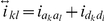and and pure additive and dominant effects may be further estimated by using the equations of and . The simulation results show that the two-step approach works well (Tables 6, 12 and 13). However, the pure epistatic effects (, and ) could not be detected with satisfactory statistical power when the sample size () and family replication number () were low (Tables 5 and 11). Therefore, a large and are needed for the detection of epistasis. To accommodate larger , suitable field experimental designs, such as split-plot design [13], [16] and block in replication [35], are desired to control for environmental error.

The F₂-based TTC design is superior to the F₂ design for the detection of main-effect and epistatic QTL when there is a small sample size and a large residual variance (Tables 3, 4, 5 and 7), and is more powerful for estimating , (or ) and especially than the F_2:3 design (Tables 4, 5 and 8). The new method may be extended to the TTC design derived from other base populations, such as RIL, BC and DH. This is because the genetic models for , and in these new TTC designs can be described in the same manner. In Tables S7, S8 and Supporting Information S3 we only presented the expected genetic values and genetic variance for , and under both the F₂ and the F_∞ metric models in the RIL-based TTC design.

The proposed approach in this study differs from the previous methods of Kearsey et al. [12], Frascaroli et al. [16], Melchinger et al. [7], [21] and Li et al. [17]. First, the former derives the linear regression models for , and and the latter makes use of ANOVA. Thus, the precondition for the former is to derive the dummy variables for each genetic effects, whereas the precondition for the latter is to obtain the expectation and expected mean squares. In the expectation and expected mean squares, if one effect is confounded by another effect, these confounded effects may be estimated together. That is the augmented effect in the above ANOVA. If there are multicollinear relationships among dummy variables, the corresponding effects cannot be estimated. However, the effect combination is estimable. That is the augmented effect in the linear regression analysis. This can explain why we construct augmented effects. Second, we consider all the main-effect QTL and all the digenic interactions in one model of Z₁ or Z₂, all the augmented additive, dominance and epistatic effects have been rightly defined, and all the pure main and epistatic effects can be unbiasedly estimated. Although in the previous studies the augmented additive and dominant effects ( and ) have been rightly defined and are clearly confounded by QTL × genetic background epistasis in the RIL-based TTC and NCIII designs [7], [21], [22], the augmented epistatic effects have been ignored. This neglect would result in a biased estimation for the augmented main effects, a larger residual variance and a lower power of QTL detection (Tables 3 and 4). In addition, with Z₃ we can estimate three types of pure epistatic effects (ad, da and dd) using two-dimensional genome scans. This differs from Melchinger et al. [21], in which only dd epistasis can be obtained.

The F₂ and F_∞ are two main metrics that are adopted for populations derived from a cross between two inbred lines. The F₂ metric is orthogonal for the F₂ population when epistatic genes are under linkage equilibrium, whereas the F_∞ metric is orthogonal for homozygous lines [28]–[30]. An orthogonal model implies that estimates of the genetic effects are consistent in a full and reduced model and is directly related to the partition of the genetic variance in the population. Using different models does not influence the detection of the main and epistatic QTL, but it does influence the estimation and interpretation of genetic effects [30]. Melchinger et al. [7], [21] and Kusterer et al. [13], [22] advocated the F₂ metric in the RIL-based NCIII and TTC designs for three reasons: (1) it has the advantage that each variance component is proportional to the sum of the squares of the corresponding genetic effects and does not involve any other type of genetic effects that could obscure their interpretation; (2) epistatic interactions by two-way ANOVAs for pairs of marker loci using was just ; and (3) with digenic epistasis, midparent heterosis involves only beside dominance effects, whereas under the F_∞ metric MPH is additionally influenced by . For F₂-based TTC design, neither F₂ nor F_∞ metric models are orthogonal (Supporting Information S2). With the Z₁ and Z₂ the newly defined parameters (, , and ) were all rightly identified and estimated by our full model methods under both metrics (Tables 3, 4, 12 and 13), and with Z₃ the pure epistatic effects (, , and ) could also be detected and well estimated under both metrics when the sample size and number of family replications were large in our simulation studies (Tables 5, 11 and 13). The differences under the two metrics may be as follows: (1) the newly defined main effects and model means are different for the Z ₁ and Z ₂ under the two models; and (2) the F₂ metric model seems to behave better than the F_∞ metric model (higher power and precision) (data not shown).

The proposed approach in this study assumes that all the QTL stand on the markers. When marker density is high, all the QTL can be detected with a high power and precision. When marker density is sparse, the QTL effects are slightly underestimated because of the recombination between QTL and its adjacent marker. To solve the issue, some virtual marker (treated as missing data) may be inserted. At this time marker imputation techniques may be used.

The drawbacks for our method may lie in two aspects: (1) with and the augmented epistatic effects ( and ) were poorly detected when their corresponding components have an equal strength in opposite directions (Tables 9, 10 and 13). This would result in biased estimate for pure aa epistatic effect, such as in Table 13, and further cause bad estimate for pure dominance effect, such as and in Table 12; and (2) The estimation error for the pure main and epistatic effects using the two-step approach seemed to be a little large. This will be studied in the future.

Supporting Information

Supporting Information S1

Statistical genetic models for mapping QTL in the TTC design under the F_∞ metric model.

(DOC)

Supporting Information S2

The expected genetic values of , and under the F₂ and the F_∞ metric models in the F₂-based TTC design.

(DOC)

Supporting Information S3

The expected genetic values of the , and values under the F_∞ and the F₂ metric models in the RIL-based TTC design.

(DOC)

Table S1

Genetic constitutions of the F₂-based TTC family means L _1i, L _2i and L _3i.

(DOC)

Table S2

Expected genetic value of L _1i family under the F₂ and the F_∞ metric models in the F₂-based TTC design.

(DOC)

Table S3

Expected genetic value of L _2i family under the F₂ and the F_∞ metric models in the F₂-based TTC design.

(DOC)

Table S4

Expected genetic value of L _3i family under the F₂ and the F_∞ metric models in the F₂-based TTC design.

(DOC)

Table S5

Expected genetic values of , and under the F₂ metric model in the F₂-based TTC design.

(DOC)

Table S6

Expected genetic values of , and under the F_∞ metric model in the F₂-based TTC design.

(DOC)

Table S7

Expected genetic values of ,and under the F₂ metric model in the RIL-based TTC design.

(DOC)

Table S8

Expected genetic values of , and under the F_∞ metric model in the RIL-based TTC design.

(DOC)

References

- 1.Carlborg Ö, Haley CS. Epistasis: too often neglected in complex trait studies. Nat Rev Genet. 2004;5:618–625. doi: 10.1038/nrg1407. [DOI] [PubMed] [Google Scholar]
- 2.Moore JH, Williams SM. Traversing the conceptual divide between biological and statistical epistasis: systems biology and a more modern synthesis. BioEssays. 2005;27:637–646. doi: 10.1002/bies.20236. [DOI] [PubMed] [Google Scholar]
- 3.Jinks JL, Jones RM. Estimation of the components of heterosis. Genetics. 1958;43:223–234. doi: 10.1093/genetics/43.2.223. [DOI] [PMC free article] [PubMed] [Google Scholar]
- 4.Yu SB, Li JX, Xu CG, Tan YF, Gao YJ, et al. Importance of epistasis as the genetic basis of heterosis in an elite rice hybrid. Proc Natl Acad Sci USA. 1997;94:9226–9231. doi: 10.1073/pnas.94.17.9226. [DOI] [PMC free article] [PubMed] [Google Scholar]
- 5.Lippman ZB, Zamir D. Heterosis: revisiting the magic. Trends in Genetics. 2006;23:60–66. doi: 10.1016/j.tig.2006.12.006. [DOI] [PubMed] [Google Scholar]
- 6.Melchinger AE, Piepho HP, Utz HF, Muminovi J, Wegenast T, et al. Genetic basis of heterosis for growth-related traits in Arabidopsis investigated by testcross progenies of near-isogenic lines reveals a significant role of epistasis. Genetics. 2007;177:1827–1837. doi: 10.1534/genetics.107.080564. [DOI] [PMC free article] [PubMed] [Google Scholar]
- 7.Melchinger AE, Utz HF, Piepho HP, Zeng ZB, Schön CC. The role of epistasis in the manifestation of heterosis: a systems-oriented approach. Genetics. 2007;177:1815–1825. doi: 10.1534/genetics.107.077537. [DOI] [PMC free article] [PubMed] [Google Scholar]
- 8.Wright S. Genic and organismic selection. Evolution. 1980;34:825–843. doi: 10.1111/j.1558-5646.1980.tb04022.x. [DOI] [PubMed] [Google Scholar]
- 9.Carson HL, Templeton AR. Genetic revolutions in relation to speciation phenomena: the founding of new populations. Annu Rev Ecol Syst. 1984;15:97–131. [Google Scholar]
- 10.Kearsey MJ, Jinks JL. A general method of detecting additive, dominance and epistatic variation for metrical traits. I. Theory. Heredity. 1968;23:403–409. doi: 10.1038/hdy.1968.52. [DOI] [PubMed] [Google Scholar]
- 11.Kearsey MJ, Pooni HS. Chapman and Hall: London; 1996. The genetical analysis of quantitative traits. [Google Scholar]
- 12.Kearsey MJ, Pooni HS, Syed NH. Genetics of quantitative traits in Arabidopsis thaliana. Heredity. 2003;91:456–464. doi: 10.1038/sj.hdy.6800306. [DOI] [PubMed] [Google Scholar]
- 13.Kusterer B, Muminovic J, Utz HF, Piepho HP, Barth S, et al. Analysis of a triple testcross design with recombinant inbred lines reveals a significant role of epistasis in heterosis for biomass-related traits in Arabidopsis. Genetics. 2007;175:2009–2017. doi: 10.1534/genetics.106.069005. [DOI] [PMC free article] [PubMed] [Google Scholar]
- 14.Jinks JL, Perkins JM. A general method for the detection of additive, dominance and epistatic components of variation III. F2 and backcross populations. Heredity. 1970;25:419–429. [Google Scholar]
- 15.Perkins JM, Jinks JL. Detection and estimation of genotype-environmental, linkage and epistatic components of variation for a metrical trait. Heredity. 1970;25:157–177. [Google Scholar]
- 16.Frascaroli E, Canè MA, Landi P, Pea G, Giabfranceschi L, et al. Classical genetic and quantitative trait loci analyses of heterosis in a maize hybrid between two elite inbred lines. Genetics. 2007;176:625–644. doi: 10.1534/genetics.106.064493. [DOI] [PMC free article] [PubMed] [Google Scholar]
- 17.Li L, Lu K, Chen Z, Mu T, Hu Z, et al. Dominance, overdominance and epistasis condition the heterosis in two heterotic rice hybrids. Genetics. 2008;180:1725–1742. doi: 10.1534/genetics.108.091942. [DOI] [PMC free article] [PubMed] [Google Scholar]
- 18.Kearsey MJ, Hyne V. QTL analysis: a simple ‘marker-regression’ approach. Theor Appl Genet. 1994;89:698–702. doi: 10.1007/BF00223708. [DOI] [PubMed] [Google Scholar]
- 19.Zeng ZB. Precision mapping of quantitative trait loci. Genetics. 1994;136:1457–1468. doi: 10.1093/genetics/136.4.1457. [DOI] [PMC free article] [PubMed] [Google Scholar]
- 20.Wang DL, Zhu J, Li ZK, Paterson AH. Mapping QTL with epistatic effects and QTL × environment interactions by mixed model approaches. Theor Appl Genet. 1999;99:1255–1264. [Google Scholar]
- 21.Melchinger AE, Utz HF, Schön CC. Genetic expectations of quantitative trait loci main and interaction effects obtained with the triple testcross design and their relevance for the analysis of heterosis. Genetics. 2008;178:2265–2274. doi: 10.1534/genetics.107.084871. [DOI] [PMC free article] [PubMed] [Google Scholar]
- 22.Kusterer B, Piepho HP, Utz HF, Schön CC, Muminovic J, et al. Heterosis for biomass-related traits in Arabidopsis investigated by quantitative trait loci analysis of the triple testcross design with recombinant inbred lines. Genetics. 2007;177:1839–1850. doi: 10.1534/genetics.107.077628. [DOI] [PMC free article] [PubMed] [Google Scholar]
- 23.Jiang C, Zeng ZB. Multiple trait analysis of genetic mapping for quantitative trait loci. Genetics. 1995;140:1111–1127. doi: 10.1093/genetics/140.3.1111. [DOI] [PMC free article] [PubMed] [Google Scholar]
- 24.Reif JC, Kusterer B, Piepho HP, Meyer RC, Altman T, et al. Unraveling epistasis with triple testcross progenies of near-isogenic lines. Genetics. 2009;181:247–257. doi: 10.1534/genetics.108.093047. [DOI] [PMC free article] [PubMed] [Google Scholar]
- 25.Zhu C, Zhang R. Efficiency of triple test cross for detecting epistasis with marker information. Heredity. 2007;98:401–410. doi: 10.1038/sj.hdy.6800956. [DOI] [PubMed] [Google Scholar]
- 26.Wang XF, Song W, Yang ZF, Wang YM, Tang ZX, et al. Improved genetic mapping of endosperm traits using NCIII and TTC designs. Journal of Heredity. 2009;100:496–500. doi: 10.1093/jhered/esp009. [DOI] [PubMed] [Google Scholar]
- 27.Lander ES, Botstein D. Mapping Mendelian factors underlying quantitative traits using RFLP linkage maps. Genetics. 1989;121:185–199. doi: 10.1093/genetics/121.1.185. [DOI] [PMC free article] [PubMed] [Google Scholar]
- 28.Kao CH, Zeng ZB. Modeling epistasis of quantitative trait loci using Cockerham's model. Genetics. 2002;160:1243–1261. doi: 10.1093/genetics/160.3.1243. [DOI] [PMC free article] [PubMed] [Google Scholar]
- 29.Yang RC. Epistasis of quantitative trait loci under different gene action models. Genetics. 2004;167:1493–1505. doi: 10.1534/genetics.103.020016. [DOI] [PMC free article] [PubMed] [Google Scholar]
- 30.Zeng ZB, Wang T, Zou W. Modeling quantitative trait loci and interpretation of models. Genetics. 2005;169:1711–1725. doi: 10.1534/genetics.104.035857. [DOI] [PMC free article] [PubMed] [Google Scholar]
- 31.Zhang YM, Xu S. A penalized maximum likelihood method for estimating epistatic effects of QTL. Heredity. 2005;95:96–104. doi: 10.1038/sj.hdy.6800702. [DOI] [PubMed] [Google Scholar]
- 32.Xu S. An empirical Bayes method for estimating epistatic effects of quantitative trait loci. Biometrics. 2007;63:513–521. doi: 10.1111/j.1541-0420.2006.00711.x. [DOI] [PubMed] [Google Scholar]
- 33.Xu S. An expectation–maximization algorithm for the Lasso estimation of quantitative trait locus effects. Heredity. 2010;105:483–494. doi: 10.1038/hdy.2009.180. [DOI] [PubMed] [Google Scholar]
- 34.Garcia AAF, Wang S, Melchinger AE, Zeng ZB. Quantitative trait loci mapping and the genetic basis of heterosis in maize and rice. Genetics. 2008;180:1707–1724. doi: 10.1534/genetics.107.082867. [DOI] [PMC free article] [PubMed] [Google Scholar]
- 35.Cockerham CC, Zeng ZB. Design III with marker loci. Genetics. 1996;143:1437–1456. doi: 10.1093/genetics/143.3.1437. [DOI] [PMC free article] [PubMed] [Google Scholar]
Associated Data
This section collects any data citations, data availability statements, or supplementary materials included in this article.
Supplementary Materials