Mean-field modeling of thalamocortical dynamics and a model-driven approach to EEG analysis

Abstract

Higher brain function depends on task-dependent information flow between cortical regions. Converging lines of evidence suggest that interactions between cortical regions and the central thalamus play a key role in establishing the dynamic patterns of functional connectivity that normally support these processes. In patients with chronic disturbances of cognitive function due to severe brain injury, dysfunction of this circuitry likely plays a crucial role in pathogenesis. However, assaying thalamocortical interactions is challenging even in healthy subjects and more so in severely impaired patients. To approach this problem, we apply a dynamical-systems approach to motivate an analysis of the electroencephalogram (EEG). We begin with a model for a single thalamocortical module [Robinson PA, Rennie CJ, Rowe DL (2002) Phys Rev E Stat Nonlin Soft Matter Phys 65:041924; Robinson PA, Rennie CJ, Wright JJ, Bourke PD (1998) Phys Rev E Stat Nonlin Soft Matter Phys 58:3557–3571]. When two such modules interact via shared thalamic inhibition, multistable behavior emerges; each mode is characterized by a different pattern of coherence between cortical regions. This observation suggests that changing patterns of cortical coherence are a hallmark of normal thalamocortical dynamics. In a preliminary study, we test this idea by analyzing the EEG of a patient with chronic brain injury, who has a marked improvement in behavior and frontal brain metabolism in response to zolpidem. The analysis shows that following zolpidem administration, changing patterns of coherence are identified between the frontal lobes and between frontal and distant brain regions. These observations support the role of the central thalamus in the organization of patterns of cortical interactions and suggest how indexes of thalamocortical dynamics can be extracted from the EEG.

The goals of this paper are to present the basis for a dynamical-systems approach to the analysis of the human electroencephalogram (EEG) and to describe a pilot study that supports its potential utility. Below we detail the sequence of considerations that forms the rationale for our approach, beginning with the biological motivations and then turning to the analytic strategy.

First, task-dependent interactions between cortical areas are essential for integrative function and organized behavior, such as working memory or forming a movement plan (1–5). Importantly, the corticocortical interactions are dynamic: They occur only at certain times in a task, and the direction of the information transfer can be task dependent (3–5). For example, an external sensory stimulus (occipitoparietal) can instruct eye movements (frontal) or an endogenous intentional signal (frontal) can drive focal attention and vision (occipitoparietal). Thus, these basic behavioral elements require corticocortical interactions, and, crucially, they must be rapidly and selectively regulated.

Second, evidence from anatomical, physiological, and clinical studies suggests that the central thalamus is key to establishing this dynamic functional connectivity (6–8). The central thalamus is dominated by the “matrix” neurons of the thalamus (6), which tend to project to superficial layers of specific sets of cortical areas and are heavily innervated by brain stem arousal systems. They are thus positioned to facilitate the activity of neurons that receive long-range connections from other cortical areas, thus supporting and modulating corticocortical interactions (6–8). Reticular neurons, although they do not directly project to cortex, also provide for coupling of distant cortical areas. This coupling occurs as a result of their inhibitory connections with thalamic relay nuclei, heavy projections to the matrix cells of the intralaminar and related “nonspecific” thalamic nuclei, and the innervation of reticular neurons by descending projections from modular cortical regions. Because these shared inhibitory interactions set up a kind of competition between thalamocortical loops, this form of coupling may allow for rapid switching between patterns of cortical connectivity, on the basis of small changes in the sensory input.

The third consideration relates to the need for modeling. Whereas the use of the EEG has several potential advantages (it is noninvasive, it can be carried out for extended periods of time even in severely ill patients, and it has good temporal resolution), it has an obvious disadvantage: The EEG registers only cortical activity. Thus, thalamic activity is not seen directly and must be inferred from its effects on cortical populations. To bridge the gap between what is readily measured and what we want to assay requires some form of modeling. Most often, the approach to EEG modeling is to use parametric modeling of the biophysics of cortical networks and the media (scalp, skull, and brain) to attempt to understand the characteristics of the EEG signal (e.g., ref. 9). However, because of the number of parameters involved, and because the EEG represents a coarse population average, solving the corresponding inverse problem is not a viable strategy. This motivates our approach to modeling: Rather than pursue a detailed, parametric approach, we instead identify the qualitative dynamical features of neural population activity that emerge from the above kinds of interactions. We focus the analysis on EEG coherences, as much of the evidence for the role of corticocortical interactions (2–5) is derived from coherences, which are also readily measured from human data.

Motivated by these considerations, the first portion of this paper determines the qualitative dynamics of a neural-population model of thalamocortical interactions. As we recently reported (10), the analysis shows that inhibitory interactions in the thalamus allow for switching between multiple modes of coherence patterns between cortical areas. This result supports the evidence reviewed above that thalamic interactions enable such shifts and, importantly, leads to a strategy for determining whether multiple modes of coherence are present in samples of human EEG. In the second portion of this paper, we apply this strategy to the EEG of a patient with chronic brain injury, who has an unusual but well-documented response to zolpidem: a marked, reversible, behavioral improvement, and a concomitant normalization of frontal metabolism. Results of the EEG analysis show that this zolpidem response is also characterized by the emergence of changing patterns of cortical coherence involving the frontal lobes, suggesting that our approach may be able to identify circuit-level dynamics that are functionally relevant.

Results

Model of Thalamocortical Dynamics.

In the first part of Results, we analyze the qualitative dynamics of a model of coupled thalamocortical modules. We focus on the consequences of shared inhibition within the thalamus; as we show, this suffices to generate multiple stable modes of cortical coherence. We then consider the effects of other kinds of coupling: shared thalamic excitation and direct cortical–cortical excitation. Our analysis shows that these forms of coupling do not contribute to multistability; rather, they work against it.

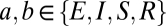
The basic building block is the population-based model of a thalamocortical module developed by Robinson and colleagues (11, 12), and our implementation of it is described in more detail in ref. 10. Briefly (see the dashed oblong in Fig. 1), the module consists of four populations of neurons: excitatory (E) and inhibitory (I) cortical neurons, a thalamic relay nucleus (S), and a thalamic reticular nucleus (R). Each population has two state variables: a mean potential V and a mean firing rate φ (s⁻¹). For each population, the mean potential V evolves in time, according to the inputs that it receives from itself and the other populations. The influence of each population b on a target population a is determined by a coupling strength and a delay , (). As illustrated in Fig. 1 and in keeping with anatomy, only some of the connections have nonzero strengths. 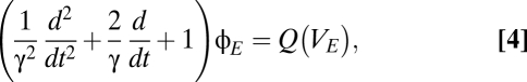Connections with positive coupling strengths are present from the cortical excitatory population, including self-excitation (), and from the relay population (); connections with negative coupling strengths are , representing inhibition within the cortex, and , representing inhibition within the thalamus. For the cortical excitatory population E and the thalamic populations S and R, the mean potential is linked to the sum of the input signals via a differential operator D,

Fig. 1.

A model of two thalamocortical modules coupled via a shared reticular nucleus. Each thalamocortical module (enclosed by a black dashed oblong) is modeled by a four-population Robinson (11, 12) system, in which the cortex is modeled by excitatory (E) and inhibitory (I) populations, and the thalamus is modeled by relay (S) and reticular (R) populations. The green and red arrows indicate local excitatory and inhibitory connections, which are assumed to have no delay. The blue arrows indicate long-range excitatory connections, characterized by a uniform propagation delay. The purple arrow indicates sensory input. The dashed arrows represent connections involving the shared thalamic reticular nucleus R_s, whose relative strength is determined by . The dotted arrows represent connections involving the unshared thalamic reticular nuclei R₁ and R₂, whose relative strength is determined by .

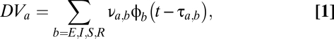where the differential operator D is given by

The potential of the cortical inhibitory population is slaved to that of the excitatory population, . The delay parameters of Eq. 1 are assumed to be zero within the cortex () and within the thalamus (); between cortex and thalamus they all have the same nonzero value, . For the differential operator of Eq. 2, the parameters α and β are chosen so that its impulse response mimics the time course of a synaptic potential.

To complete the description of the model, it is necessary to specify how the firing rate of a population depends on its mean potential . For the populations with relatively compact neurons, in which signal propagation is limited , this relationship is assumed to be a sigmoidal function:

For the cortical excitatory population , potentials are assumed to propagate in a wave-like fashion. For spatially uniform solutions (the only ones we consider here), this assumption leads to

where γ is the ratio of the propagation velocity to mean axonal length. In the analysis below, we consider both the qualitative nature of the solutions to the system of Eqs. 1–4 and the spectral characteristic of solutions in which the relay population S is driven by a random input,

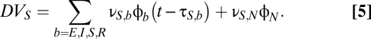The random input term, which represents sensory input, is modeled as white noise, 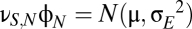of mean μ and spectral density . For numerical integration with step size , the input is generated by independent draws from a Gaussian of SD .

Qualitative Behavior of Coupled Thalamocortical Modules.

Eqs. 1–4 constitute a population-level model of a single thalamocortical module. With this as our starting point, we now proceed to determine the dynamics of coupled modules. We consider two identical modules (Fig. 1) and designate their component populations as E_j, I_j, S_j, and R_j (). The specific parameter values we use are those for which the spectral characteristics of the excitatory cortical potential, , match those of the human EEG in different behavioral states: eyes-open alert (EO), eyes-closed alert (EC), light sleep (S2), and deep sleep (S3) (see ref. 10 for parameter values). As described below, we probe the effects of coupling by introducing populations that are shared between the modules, along with parameters and that specify the connection strengths for the shared populations () and the unshared populations () in terms of the single-module connectivity parameters .

Thus, to model coupling via the reticular nucleus, we introduce a shared reticular population, R_s. As shown in Fig. 1, its connections (dashed arrows) correspond to those of the unshared populations R₁ and R₂: It receives input from both cortical excitatory populations E₁ and E₂ and inhibits the two relay populations S₁ and S₂. Its connection strengths are specified in terms of those of the basic module: 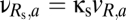(nonzero for ). The connection strengths for the unshared populations R₁ and R₂ (dotted arrows in Fig. 1) are given by ; we allow for the factor so that we can add the shared population without necessarily changing the total size of the reticular populations. Note that corresponds to two uncoupled modules with standard parameters, corresponds to two such modules whose reticular component is entirely shared, and the line corresponds to intermediate configurations, in which a portion of the reticular population is shared.

At this point, the task at hand is to determine the qualitative behavior of this coupled system, as a function of the parameters and . We use a standard approach for doing this (see ref. 10 for details) that makes use of the fact that the system defined by Eqs. 1–4 is a delay differential equation. The result of the analysis is a bifurcation diagram, i.e., a parcellation of the plane into regions, each of which corresponds to a different qualitative behavior of the system (see, for example, Fig. 2). The bifurcation diagram thus concisely characterizes the different kinds of qualitative behaviors that the system can manifest. Below we describe the bifurcation diagrams that emerge from the above system and several variants of that system.

Fig. 2.

Bifurcation diagram for the pair of coupled thalamocortical modules illustrated in Fig. 1. Dotted black curve: boundary of the physiological regime. Blue curve: fold bifurcation, below which a winner-take-all (WTA) mode exists. Black curve: pitchfork bifurcation, below which the symmetric mode is unstable. Red curve, Hopf bifurcation, below which the symmetric mode is oscillatory. Green curve: Hopf bifurcation, below which the WTA solutions are oscillatory. Note that in all parts of the gray region, symmetric and WTA modes are both stable. The purple line segment serves as an anchor for the region explored in Fig. 4. This figure was redrawn, with permission, from Drover et al. (10), figure 6A.

Inhibitory Coupling via the Central Thalamus.

The bifurcation diagram for the coupled system of Fig. 1 (with the parameter set of the EO state) is shown in Fig. 2. As described above, this diagram summarizes the way that the qualitative dynamics of the coupled system depend on the parameters of interest: , the strength of the shared reticular component, and , the strength of the unshared reticular component. We begin at the vertical axis (where the modules are independent) and sweep down to the horizontal axis (where the modules are maximally coupled).

Along the vertical axis, , behavior is simple. At , which corresponds to the standard level of the reticular inhibition in the EO parameter set, there is a single, stable fixed point. As the strength of the reticular inhibition decreases below the red curve, the system enters an oscillatory regime. This change in behavior corresponds to a transition from a conjugate pair of complex conjugate roots of the characteristic equation with a negative real part to a pair with a positive real part, i.e., a Hopf bifurcation (10). When inhibition decreases further, below the dotted black curve in Fig. 2, the system enters a mode in which activity in the excitatory populations saturates at high levels; this region is a nonphysiologic parameter range and we consider it no further.

Near the vertical axis ( small), behavior remains simple. Because coupling is weak, the modules act as if they are uncoupled, and the only effect of coupling is to synchronize their activity. We designate this case, where both modules maintain similar activity, as the “symmetric” mode.

Additional behaviors emerge toward the middle of the diagram, as the coupling between the modules increases. When is sufficiently high, activity in one module can drive down the activity in another module. This “winner-take-all” (WTA) behavior, in which one module has a high level of activity, corresponds to new fixed points. These solutions arise along a fold bifurcation, which is indicated by the blue curve in Fig. 2. Moreover, depending on the combined values of and , the WTA solutions themselves can become oscillatory; this transition is indicated by the green curve, another Hopf bifurcation, in Fig. 2.

The most interesting aspect of the system's dynamics is that there is an overlap between the domain in which the symmetric solution is stable and the domain in which WTA solutions are present—the gray region in Fig. 2. This overlap occurs because the loss of stability of the symmetric solution and the formation of the WTA solution occur via separate mechanisms. The symmetric solution loses stability by a pitchfork bifurcation, which corresponds to the black curve in Fig. 2; in contrast, the WTA solution (mentioned above) is generated by a fold bifurcation (the blue curve in Fig. 2). Between these two bifurcation curves is a region (shaded gray in Fig. 2) in which the WTA solutions have emerged, and the symmetric solution has not yet become unstable. This overlap includes subregions in which the symmetric solution is oscillatory (below the red curve) and in which the WTA solutions are oscillatory (below the green curve).

Finally, when shared inhibition becomes overwhelming (near the horizontal axis), the behavior of the system again simplifies: Within the physiologic range, only the WTA behavior is stable, and this stability can be either oscillatory (to the left of the red curve in Fig. 2) or nonoscillatory (to its right.)

In Drover et al. (10), we confirmed this mathematical analysis via numerical simulations (forward integration of the system, with a driving noise term, as in Eq. 5). We also showed that the multistable behavior was found not only for the EO parameter set (as in Fig. 2), but also for the EC parameter set and for the light sleep parameter set (S2). Interestingly, although this behavior is robust, it is not universal: the deep-sleep parameter set (S3) does not manifest WTA behavior. The mechanism of emergence of the multistable behavior is also discussed in Drover et al. (10).

Excitatory Coupling via the Thalamic Projections.

We now extend the above analysis to include another form of coupling that is suggested by the anatomy: joint activation of both cortical regions by projections from the intralaminar nuclei. To model this form of coupling, we add another component: a thalamic nucleus L that projects to both cortical populations E₁ and E₂ (Fig. 3). Because this nucleus receives its own excitation and projects directly to both cortical populations, it provides a form of coupling that is distinct from the shared inhibition considered above.

Fig. 3.

Addition of shared thalamic excitation to the model of Fig. 1. The heavy dashed arrows are connections involving L, which represents a thalamic nucleus that projects to two cortical regions. Thin arrows represent connections already present in the model of Fig. 1; see Fig. 1 caption for color conventions.

To specify the model without adding multiple new parameters, the connection parameters of the population L are assumed to be a scaled version of the connection parameters of the relay nuclei S₁ and S₂: , , , and .

Fig. 4A shows how excitatory coupling interacts with coupling via shared inhibition. Specifically, it is the bifurcation diagram in the (, ) plane, with , a value that includes the multistable region of Fig. 2. The horizontal () axis of Fig. 4A thus corresponds to a horizontal line that traverses the multistable region (, indicated in purple). As Fig. 4A shows, increasing the shared excitation () narrows the region between the fold bifurcation (blue) and the pitchfork bifurcation (black), thus diminishing the region in which multistability is present. For sufficiently high values of shared excitation (), the fold bifurcation merges into the pitchfork, and mulitstability no longer occurs.

Fig. 4.

The effect of other forms of coupling on the region of multistability. (A) Shared excitatory coupling via the thalamus (parameterized by ) reduces the region of multistability, which corresponds to the parameter values between the blue curve (the fold bifurcation) and the black curve (the pitchfork bifurcation). (B) The effect of direct corticocortical coupling. When coupling has a net excitatory character (), the region of multistability (between the two bifurcation curves) is diminished; when coupling has a net inhibitory character (), the region is enlarged. In both A and B, the purple line segment is identical to the purple line segment within the bifurcation diagram of Fig. 2, at and .

In sum, coupling via shared excitatory input does not produce multistability and, in fact, tends to diminish the range of parameter values and for which multistability occurs.

Coupling at the Cortical Level.

As is well known, the long axons of layer III pyramidal neurons provide a means for direct corticocortical interactions (13). Anatomically, these connections can be interhemispheric (via the corpus callosum) or intrahemispheric (connecting distant regions via the deep white matter or adjacent regions via the U-fibers). To model their effects on dynamics, we included direct corticocortical excitatory connectivity, formalized by coupling constants and . We parameterize the strength of this coupling by , its strength relative to cortical self-excitation, and, for simplicity, we assume that this coupling is symmetric: and .

Fig. 4B shows the effects of adding this form of coupling. The line indicates the behavior of the baseline system with shared reticular coupling (, ); the upper half of the plot indicates increasing amounts of excitatory corticocortical coupling, . As is the case for shared thalamic excitation (Fig. 4A), corticocortical coupling narrows the region between the fold bifurcation and the pitchfork bifurcation, decreasing the region of multistability. Of note, this behavior does not depend on the size of the corticocortical conduction delay, because the relevant bifurcations are folds and pitchforks (10). Thus, excitatory coupling at the cortical level, like excitatory coupling at the thalamic level (Fig. 4A), stabilizes the symmetric mode of behavior and reduces the domain of multistability.

Finally, we consider the possibility that the corticocortical projection neurons, although excitatory in nature, terminate primarily on inhibitory interneurons and thus have a net inhibitory effect (e.g., ref. 13). A simple way to model the consequences of this possibility (without adding further parameters) is to allow the coupling constant to be negative. When this is done, the domain of multistability increases (, lower half of Fig. 4B). That is, viewed as a perturbation on the basic model of thalamocortical dynamics (Fig. 1), net inhibitory corticocortical coupling enlarges the domain of multistability, whereas net excitatory corticocortical coupling diminishes this domain. Moreover, if is sufficiently negative, multistability can occur even in the absence of shared inhibitory coupling in the thalamus ().

From Model to EEG Analysis Strategy.

Our next step is to use the inferences from the above modeling study to motivate a strategy for EEG analysis. To do this, we first need to synthesize the bifurcation analysis into an understanding of the global behavior of the model. As we showed above, when thalamocortical modules are coupled via partially shared inhibition, they will exhibit multiple modes of stable behavior: a symmetric mode and two WTA modes in which one module's activity drives down the other. Each of these modes is associated with different stable solutions of the model equations, so we anticipate that these different modes (symmetric and WTA modes) will have qualitatively different spectral characteristics. Each of the steady-state solutions (fixed points) corresponds to a distinct basin of attraction, within which unperturbed solutions converge to the fixed point. We therefore anticipate that the system will remain in one of these states, until the noise excitation is sufficiently large to cause a jump into one of the other states.

As shown in Drover et al. (10), these anticipations are confirmed by numerical solution of the original delay-differential equations. Specifically, the activity levels of populations make abrupt transitions between discrete modes of behavior (Fig. 5A), and within these modes, the spectral characteristics determined analytically from the linearized model equations correspond closely to those obtained by numerical integration of the original equations excited by white noise (Fig. 5B). This correspondence holds for each of the modeled populations; we illustrate it for the excitatory cortical populations and , because our goal is to connect model behavior with the EEG.

Fig. 5.

The bifurcation analysis captures the dynamical features of the population model. (A) Numerical solutions of the equations undergo the predicted abrupt transitions between modes. Blue trace, ; red trace, . As predicted by the bifurcation analysis, there are abrupt transitions between a symmetric mode in which the two signals are largely synchronized and winner-take-all (WTA) modes in which one cortical region dominates the other. (B) The spectral characteristics of these modes determined by numerical integration (black) closely match those determined from the linearized equations (green). Parameters are taken from the EO state, with and . This figure was redrawn, with permission, from Drover et al. (10), figures 4 and 5.

In motivating a strategy for EEG analysis, we focus on the presence of these spontaneous transitions between states with distinct coherence patterns. The rationale is that this feature is robust: It emerges from a qualitative analysis of the behavior of the system, and, as we showed (10), it is not specific to a particular choice of parameter values. In contrast, the position of the spectral peaks (Fig. 5B) will be highly dependent on the particular choice of time constants and connection strengths. Similarly, we do not attempt to make use of the frequency of transitions between the states or their dwell times, because this will depend sensitively on the size of the noise excitation. Given the obvious simplified nature of the model, these robustness considerations are crucial.

If it were possible to obtain artifact-free direct-coupled (DC) recordings of EEG for long periods of time (analogous to the time series shown in Fig. 5A for and ), then we could simply inspect these time series for abrupt transitions and, hence, evidence of multistability. However, such recordings are not possible—especially in recordings from patients who are unable to cooperate—so we are driven to adopt a somewhat more indirect approach to detect multistability that can be applied to brief epochs of recordings and does not require DC recording.

Fig. 6 illustrates this strategy, first with model data and then applied to clinical EEG. In Fig. 6A, we analyze 300 s of the model outputs and . Because these are continuous, noise-free data, the transitions between modes are readily apparent from the abrupt changes in the spectrograms and coherograms. To develop an approach that will also work when only brief segments of data are available, we begin by looking for structure in the pattern of variation of the coherogram, by applying principal components analysis to it:

Fig. 6.

Identification of fluctuations of coherence modes in EEG data. (A) Spectrograms and coherograms from model simulations (Left) and surrogate data (Right). Below the coherogram is the time course of the first principal component and the histogram of these values. (B) A parallel analysis of patient EEG recordings at F7 and F8 (Laplacian derivation) under baseline conditions (Left) and following zolpidem administration (Right). The vertical bars superimposed on the spectrograms and coherograms indicate the subdivision of the data into epochs. Calibration bars apply to all horizontal axes in A and B and to the vertical axis for the first principal component; full time axes are 300 s (A), 93 s (B, Left), and 240 s (B, Right). C summarizes the evidence for multimodality in the coherences measured between multiple electrode pairs (significance level indicated by color: red, ; orange, ; yellow, ; L, R, A, and P indicate left, right, anterior, and posterior, respectively; see key for 10–20 system electrode designations) and ¹⁸FDG-PET images of metabolic activity [standardized uptake values (ref. 30) indicated by color]. Note that following zolpidem, multimodality appears in the frontal channels, along with an increase in frontal metabolic activity.

Here, is the coherogram at frequency f and time t, and each term on the right-hand side is chosen in a stepwise fashion to provide the best possible approximation to . Thus, the frequency dependence of the first principal component, , indicates the pattern of fluctuation that accounts for the most variance, and its temporal multiplier, , indicates the weight of this factor in at time t. As Fig. 6A (Left) shows, the temporal multiplier for the first principal component, , tracks the abrupt changes in modes. Because these mode transitions are discrete, the distribution of values of is bimodal. Conversely, multimodality of the distribution is an indicator that the coherence tended to dwell in discrete states. As a control, we apply an identical analysis to surrogate data, constructed to be stationary Gaussian processes with the same spectra as and (Fig. 6A, Right). Here, there is no evident variation in the spectrogram across time, and the distribution of is unimodal.

Crucially, these analysis procedures (principal components analysis, followed by examination of the distribution of values of the temporal multipliers corresponding to the principal components) can be applied to piecewise data and are thus applicable to clinical EEG as well. To provide an objective test of whether the distribution of a temporal multiplier is significantly multimodal, we apply the Hartigan dip statistic (14) and compare its value for the actual data to that of 200 Gaussian surrogates. In the example below, we consider only the first principal component, because it is the only component for which the fraction of the variance explained was substantially more than expected from surrogate data (∼20% excess).

Fig. 6 B and C shows the results of applying this analysis to the EEG of a patient with severe brain damage, in whom marked improvements in behavior and brain function were reliably induced by oral zolpidem administration (15). This is an unusual but well-documented phenomenon (16, 17) that would allow us to carry out a within-patient comparison and to correlate the findings with regional changes in brain metabolism (see Materials and Methods for clinical details). Fig. 6B shows the spectrograms and coherograms obtained from the EEG recorded at a pair of frontal channels. At baseline (Fig. 6B, Left), there were only minimal fluctuations in the EEG spectra, and the distribution of did not differ significantly from unimodality (P > 0.1), indicating that no fluctuations in dynamics were detected. Following zolpidem (Fig. 6B, Right), there were multiple abrupt fluctuations in the spectrogram, amounting to changes in power of more than a factor of 10, and the distribution of was significantly multimodal, P < 0.01. Fig. 6C summarizes this analysis for multiple pairs of EEG channels. Under baseline conditions (Fig. 6C, Left), there was tendency toward a departure from unimodality at central locations (0.05 ≤ P < 0.1). Following zolpidem (Fig. 6C, Right), there was evidence for fluctuations of bifrontal coherence (as in Fig. 6B) and, especially on the right, for fronto-occipital coherence. Along with the emergence of frontal fluctuations in coherence, an ¹⁸FDG PET study showed that zolpidem induced a normalization in cerebral metabolism, primarily involving the frontal lobes, the striatum, and the thalamus.

Discussion

In the first part of the Results, we have characterized the qualitative behavior of a population-level model of thalamocortical dynamics. The model consists of two thalamocortical modules (11, 12) that are coupled via shared inhibition in the reticular thalamus (Fig. 1). Our main finding (10) is that shared reticular inhibition provides for multiple modes of stable coherence patterns: a symmetric mode in which cortical regions are synchronously active and two winner-take-all modes in which each cortical region drives the other (Figs. 2 and 5). Because these several modes constitute basins of attraction that are simultaneously present, small fluctuations in thalamic input can cause the dynamics to switch rapidly from one mode to another (Fig. 5). This kind of behavior is specifically due to coupling via inhibition; coupling via shared excitation from thalamic relay nuclei (Fig. 3) or direct corticocortical excitatory coupling reduces and eventually extinguishes this multistability (Fig. 4).

The conclusions of the modeling studies, that central thalamic interactions allow for cortical dynamics to switch rapidly from one mode to another, along with several lines of evidence that cognitive operations are associated with specific patterns of corticocortical coherence (2–5), support the notion that the central thalamus (6–8) is crucially important for establishing dynamic functional connectivity patterns required for cognitive function.

It is important to stress that these conclusions are based on a mathematical analysis of the dynamics, rather than a numerical simulation, because this approach broadens the relevance of the conclusions. From a rigorous point of view, this analysis guarantees their validity in a range of parameter values surrounding the particular ones chosen for illustration. For example, this analysis allows us to conclude that multistability will be present even for cortical modules that are not identical. More broadly (but without a rigorous guarantee), the qualitative nature of our analysis makes it likely that our conclusions concerning its behavior are biologically relevant even though the model itself is oversimplified. For discussion of some simplifications made—both at the cellular and at the network level—see ref. 10.

The present analysis also suggests a way of identifying “fingerprints” of thalamic activity in the surface EEG. Coherence of population activity between widely separated cortical regions is readily measurable from the surface EEG, and the model suggests that fluctuations of these coherence patterns rely on thalamic interactions between cortical modules. With this in mind, we analyzed the coherence patterns in a patient in whom marked improvement in brain function could be reliably induced by zolpidem. As we showed (Fig. 6), this improvement was associated with evidence for multiple modes of coherence in frontal regions, corresponding to the regions of greatest metabolic normalization.

This analysis is presented as evidence that analysis of coherence patterns is practical even in the very challenging setting of severe brain injury and as preliminary evidence of its utility. We chose a patient who demonstrated the “zolpidem effect” (16, 17) because it allowed us to carry out a within-patient comparison and to correlate our findings with metabolic imaging. However, we emphasize both its preliminary nature (it is an “N = 1” analysis) and that we make no claim that it is specific to the zolpidem effect.

Although the underlying mechanisms of the response to zolpidem are not known, direct action of zolpidem on GABA-A α-1 receptors in the globus pallidus (18, 19) and inhibitory interneuronal networks of the anterior forebrain (20) has been proposed to underlie a reactivation of thalamocortical and thalamostriatal outflow increasing synaptic background activity and normalizing firing patterns in neocortical, striatal, and thalamic neurons. We anticipate that the appearance of coherence fluctuations in the patient shown in Fig. 6B reflects a general phenomenon associated with the observed normalization of cerebral metabolism and behavior, rather than a zolpidem-specific effect.

Broad application of coherence fluctuations to the study of the injured brain will be challenging, as this measure is likely to be sensitive to detailed functional interactions that may be impacted by many confounding factors such as medications, heterogeneity of underlying etiologies of brain injury, and patterns of structural disconnection. Nonetheless, the present study—which mitigated these factors by a within-patient design—suggests that further exploration is warranted and that tracking of coherence fluctuations in patients recovering from severe brain injuries may yield important clues to pathophysiologic mechanisms at the circuit level.

Materials and Methods

Bifurcation Analysis of Population Models.

Characterization of the qualitative behavior of the model equations, a system of delay differential equations, was carried out by standard methods (21, 22). Roots of the transcendental equations required for these calculations were determined numerically by Newton's method, implemented using Octave (23). Time series were calculated using XPPAUT (24).

Clinical Data.

The patient EEG data were collected from a 32-y-old male (15) emerged from minimally conscious state (25), as a result of severe hypoxic injury following near drowning, 9 y before evaluation. The behavioral response to zolpidem was discovered incidentally by the patient's mother and was detailed during an inpatient clinical research evaluation. Briefly, the patient's baseline neurologic status consisted of a spastic left hemiparesis with flexor posturing, accompanied by dysarthria, dysphagia, a 1- to 1.5-Hz resting tremor in the right arm, and extensor posturing in both legs. Following 10 mg zolpidem, verbal fluency and articulation improved, oral feeding became possible, spasticity was reduced, and the resting tremor was eliminated, enabling smooth, goal-directed movements and manipulation of objects. Anatomical MRI demonstrated a left thalamic lesion, and ¹⁸FDG-PET showed that global metabolism increased more than twofold following zolpidem, with the largest increases in the frontal lobes (139–183%), the striatum (156%), and the thalamus (128–148%).

EEG Acquisition and Analysis.

During the inpatient evaluation, the EEG was recorded via silver-cup electrodes ( impedance) and digitized at 200 Hz following amplification and 80 Hz lowpass anti-aliasing filtering (XLTEK; Natus Medical). With the aid of simultaneously recorded video, multiple artifact-free 3-s segments were selected from a period prior to (31 segments over a 25-min period) and 20 min following (79 segments over a 33-min period) oral zolpidem administration. Data were linearly reformatted from the 31 recorded channels (augmented 10–20 system, FCz reference) into Laplacian montage at 19 locations (Fp1, F3, C3, P3, O1, F7, T3, T5, Fp2, F4, C4, P4, O2, F8, T4, T6, Fz, Cz, and Pz), using the Hjorth approximation (26), and linearly detrended within each 3-s segment. From these 19 locations, coherences were calculated at 17 pairs (8 interhemispheric, 9 longitudinal), chosen to provide efficient coverage of the head while minimizing pairs that shared a common lead (27). For each selected pair of Laplacian channels, spectrograms and coherograms were calculated via the multitaper method (28, 29), with nonoverlapping 1-seg analysis windows and five tapers. Principal components analysis was applied to the resulting time-frequency decompositions, and the Hartigan dip test (14) was used to assay the degree of multimodality of the resulting weights. To assess statistical significance of the Hartigan dip parameter, we repeated these calculations on Gaussian surrogate data, created to have spectra and cross-spectra that matched those of the original data and segmented into similar epochs. These surrogates were created by choosing, at each temporal frequency, sine and cosine Fourier amplitudes from the multivariate Gaussian distribution. All calculations were carried out with custom software (Matlab; MathWorks), which invoked the Chronux toolkit (28) for spectral analysis.

The above evaluations were carried out following informed consent obtained from the patient's legally authorized representative, under protocols approved by the Weill Cornell Medical College Institutional Review Board.

References

- 1.Zaksas D, Pasternak T. Directional signals in the prefrontal cortex and in area MT during a working memory for visual motion task. J Neurosci. 2006;26:11726–11742. doi: 10.1523/JNEUROSCI.3420-06.2006. [DOI] [PMC free article] [PubMed] [Google Scholar]
- 2.Rodriguez E, et al. Perception's shadow: Long-distance synchronization of human brain activity. Nature. 1999;397:430–433. doi: 10.1038/17120. [DOI] [PubMed] [Google Scholar]
- 3.Pesaran B, Nelson MJ, Andersen RA. Free choice activates a decision circuit between frontal and parietal cortex. Nature. 2008;453:406–409. doi: 10.1038/nature06849. [DOI] [PMC free article] [PubMed] [Google Scholar]
- 4.Pesaran B, Pezaris JS, Sahani M, Mitra PP, Andersen RA. Temporal structure in neuronal activity during working memory in macaque parietal cortex. Nat Neurosci. 2002;5:805–811. doi: 10.1038/nn890. [DOI] [PubMed] [Google Scholar]
- 5.Womelsdorf T, Fries P. The role of neuronal synchronization in selective attention. Curr Opin Neurobiol. 2007;17:154–160. doi: 10.1016/j.conb.2007.02.002. [DOI] [PubMed] [Google Scholar]
- 6.Jones EG. The thalamic matrix and thalamocortical synchrony. Trends Neurosci. 2001;24:595–601. doi: 10.1016/s0166-2236(00)01922-6. [DOI] [PubMed] [Google Scholar]
- 7.Purpura K, Schiff N. The thalamic intralaminar nuclei: A role in visual awareness. Neuroscientist. 1997;3:314–321. [Google Scholar]
- 8.Schiff ND. Central thalamic contributions to arousal regulation and neurological disorders of consciousness. Ann N Y Acad Sci. 2008;1129:105–118. doi: 10.1196/annals.1417.029. [DOI] [PubMed] [Google Scholar]
- 9.Nunez PL, Srinivasan R. Electric Fields of the Brain: The Neurophysics of EEG. New York: Oxford Univ Press; 2006. [Google Scholar]
- 10.Drover JD, Schiff ND, Victor JD. Dynamics of coupled thalamocortical modules. J Comput Neurosci. 2010;28:605–616. doi: 10.1007/s10827-010-0244-5. [DOI] [PubMed] [Google Scholar]
- 11.Robinson PA, Rennie CJ, Wright JJ, Bourke PD. Steady states and global dynamics of electrical activity in the cerebral cortex. Phys Rev E Stat Nonlin Soft Matter Phys. 1998;58:3557–3571. [Google Scholar]
- 12.Robinson PA, Rennie CJ, Rowe DL. Dynamics of large-scale brain activity in normal arousal states and epileptic seizures. Phys Rev E Stat Nonlin Soft Matter Phys. 2002;65:041924. doi: 10.1103/PhysRevE.65.041924. [DOI] [PubMed] [Google Scholar]
- 13.David O, Friston KJ. A neural mass model for MEG/EEG: Coupling and neuronal dynamics. Neuroimage. 2003;20:1743–1755. doi: 10.1016/j.neuroimage.2003.07.015. [DOI] [PubMed] [Google Scholar]
- 14.Hartigan JA, Hartigan PM. The dip test of unimodality. Ann Stat. 1985;13:70–84. [Google Scholar]
- 15.Williams ST, et al. Society for Neuroscience. Chicago: Society for Neuroscience; 2009. Quantitative neurophysiologic characterization of a paradoxical response to zolpidem in a severely brain-injured human subject. Program 541.6. [Google Scholar]
- 16.Whyte J, Myers R. Incidence of clinically significant responses to zolpidem among patients with disorders of consciousness: A preliminary placebo controlled trial. Am J Phys Med Rehabil. 2009;88:410–418. doi: 10.1097/PHM.0b013e3181a0e3a0. [DOI] [PubMed] [Google Scholar]
- 17.Brefel-Courbon C, et al. Clinical and imaging evidence of zolpidem effect in hypoxic encephalopathy. Ann Neurol. 2007;62:102–105. doi: 10.1002/ana.21110. [DOI] [PubMed] [Google Scholar]
- 18.Schiff ND, Posner JB. Another “Awakenings”. Ann Neurol. 2007;62:5–7. doi: 10.1002/ana.21158. [DOI] [PubMed] [Google Scholar]
- 19.Schiff ND. Recovery of consciousness after brain injury: A mesocircuit hypothesis. Trends Neurosci. 2010;33:1–9. doi: 10.1016/j.tins.2009.11.002. [DOI] [PMC free article] [PubMed] [Google Scholar]
- 20.Brown EN, Lydic R, Schiff ND. General anesthesia, sleep, and coma. N Engl J Med. 2010;363:2638–2650. doi: 10.1056/NEJMra0808281. [DOI] [PMC free article] [PubMed] [Google Scholar]
- 21.Wiggins S. Introduction to Applied Nonlinear Dynamical Systems and Chaos. Heidelberg: Springer; 1990. [Google Scholar]
- 22.Engelborghs K, Luzyanina T, Roose D. Numerical bifurcation analysis of delay differential equations using ddebiftool. ACM Trans Math Softw. 2002;28:361–385. doi: 10.1007/s002850000072. [DOI] [PubMed] [Google Scholar]
- 23.Eaton JW, Bateman D, Hauberg S. GNU Octave Manual. Network Theory Limited, Bristol, UK; 2002. [Google Scholar]
- 24.Ermentrout GB. Simulating, Analyzing, and Animating Dynamical Systems: A Guide to XPPAUT for Researchers and Students. Philadelphia: Society for Industrial and Applied Mathematics; 2002. [Google Scholar]
- 25.Giacino JT, et al. The minimally conscious state: Definition and diagnostic criteria. Neurology. 2002;58:349–353. doi: 10.1212/wnl.58.3.349. [DOI] [PubMed] [Google Scholar]
- 26.Hjorth B. Source derivation simplifies topographical EEG interpretation. Am J EEG Technol. 1980;20:121–132. [Google Scholar]
- 27.Nunez PL, et al. EEG coherency. I: Statistics, reference electrode, volume conduction, Laplacians, cortical imaging, and interpretation at multiple scales. Electroencephalogr Clin Neurophysiol. 1997;103:499–515. doi: 10.1016/s0013-4694(97)00066-7. [DOI] [PubMed] [Google Scholar]
- 28.Mitra PP, Bokil H. Observed Brain Dynamics. New York: Oxford Univ Press; 2008. [Google Scholar]
- 29.Thomson DJ. Spectrum estimation and harmonic analysis. Proc IEEE. 1982;70:1055–1096. [Google Scholar]
- 30.Thie JA. Understanding the standardized uptake value, its methods, and implications for usage. J Nucl Med. 2004;45:1431–1434. [PubMed] [Google Scholar]