Inference for causal interactions for continuous exposures under dichotomization

Summary

Dichotomization of continuous exposure variables is a common practice in medical and epidemiologic research. The practice has been cautioned against on the grounds of efficiency and bias. Here we consider the consequences of dichotomization of a continuous covariate for the study of interactions. We show that when a continuous exposure has been dichotomized certain inferences concerning causal interactions can be drawn with regard to the original continuous exposure scale. Within the context of interaction analyses dichotomization and the use of the results in this paper can furthermore help prevent incorrect conclusions about the presence of interactions that result simply from erroneous modeling of the exposure variables. By considering different dichotomization points one can gain considerable insight concerning the presence of causal interaction between exposures at different levels. The results in this paper are applied to a study of the interactive effects between smoking and arsensic exposure from well water in producing skin lesions.

1. Introduction

Dichotomization of continuous exposure variables is a common practice in medical and epidemiologic research. Dichotomization is generally done so as to simplify the analysis of association between exposure and the outcome. The current statistical literature assessing the practice of dichotomization is largely negative, pointing out the adverse consequence of dichotomization for either efficiency (Cox, 1957; Cohen, 1983; Delpizzo and Borghes, 1995; Weinberg, 1995; MacCallum et al., 2002; Senn, 2003; Royston, Altman and Sauerbrei, 2006; Fedorov, Mannino and Zhang, 2009) or bias (Gustafson and Le, 2002; Royston et al., 2006). In this paper we extend the existing literature on dichotomization in two respects: first, we consider not simply the implications for dichotomization for main effects but instead we focus here on the implications of dichotomization for the analysis of interactions; second, in contrast to prior literature, we actually provide some positive results. We show that in interaction analyses, when a continuous exposure has been dichotomized and one applies standard tests for interaction for the dichotomized exposure, one can in fact draw useful conclusions about causal interactions with regard to the underlying continuous scale.

The remainder of this paper is structured as follows. In section 2 we review certain tests for interaction analyses generally and for causal interactions specifically. In section 3 we give two results concerning the conclusions one can draw about interaction with respect to the underlying continuous exposure when one applies the interaction tests to a dichotomized version of the exposure. In section 4 we apply the results from section 3 along with a marginal structural model analysis technique (Robins, Hernán and Brumback, 2000; VanderWeele, Vansteelandt and Robins, 2010) to draw conclusions about possible causal interaction between the effects of smoking and exposure to arsenic in well water on the development of pre-malignant skin lesions. In section 5 we offer some concluding remarks and discuss possible directions for future research.

2. Interaction Tests for Dichotomous Exposures

In this section we review some definitions, tests and results for interaction analyses when the two exposures of interest, X₁ and X₂ say, are both binary. We assume throughout that our outcome D of interest is also binary. In the following section we will consider the setting in which one exposure X₁ is binary but the other exposure V is continuous; we will consider the implications of applying the interaction tests for binary exposures presented in this section to the case when the continuous exposure V has been dichotomized at some arbitrary cutoff h so that X₂ is defined by X₂ = 1(V > h) where 1(·) denotes an indicator function.

Let p_x1x2 = P(D = 1∣X₁ = x₁, X₂ = x₂). The standard test for an interaction on the additive scale is

$$p_{11}-p_{10}-p_{01}+p_{00}>0.$$

If this inequality is satisfied then the effects of X₁ and X₂ together exceed the sum of the effects of X₁ and X₂ considered individually i.e. (p₁₁−p₀₀) > (p₁₀−p₀₀) + (p₀₁−p₀₀). If C denotes some set of covariates we might also consider the conditional version of this interaction test. If we let p_x1x2c = P(D = 1∣X₁ = x₁, X₂ = x₂, C = c) then the test for a conditional interaction on the additive scale within stratum C = c is p_11c − p_10c − p_01c + p_00c > 0. Further comments about the causal interpretation of the inequality is given below.

In this paper we will be principally interested in conclusions about causal interactions such that for some individuals the effects of two exposure interact so that the outcome is present when both exposures occur but is absent if just one or the other of the exposures occur. In this section, we will consider causal notions of interaction for binary exposures and how to test for such interactions. In the following section we will consider more general notions for causal interaction between continuous exposures and binary exposures.

Let Ω denote the sample space of individuals and let D_x1x2 (ω) denote the counterfactual outcome (or potential outcome, Neyman, 1923; Rubin, 1974) for individual ω if, possibly contrary to fact, X₁ had been set to x₁ and X₂ had been set to x₂. Let C denote some set of covariates. We will say the effects of X₁ and X₂ on D are unconfounded conditional on C if for all x₁, x₂, D_x1x2 is independent of (X₁, X₂) conditional on c. If the effects of X₁ and X₂ on D are unconfounded conditional on C then we have that for all x₁, x₂, c,

$$P(D_{x_1{x}_2}=1\mid \mathbf{\text{C}}=\mathbf{\text{c}})=P(D=1\mid X_1=x_1,X_2=x_2,\mathbf{\text{C}}=\mathbf{\text{c}})$$

so that within strata of the covariates C, the observed association between D and (X₁, X₂) reflect the actual causal effects of what would happen under intervention on X₁ and X₂. Note we assume that the consistency assumption holds that if X₁(ω) = x₁, X₂(ω) = x₂ then D_x1x2 = D(ω) (Robins, 1986; cf. VanderWeele, 2009a).

VanderWeele and Robins (2008) said that a sufficient cause interaction was present between X₁ and X₂ if there was some individual ω such that D₁₁(ω) = 1 but D₁₀(ω) = D₀₁(ω) = 0 and they showed that if there were such an individual then synergism within Rothman's sufficient cause framework (Rothman, 1976) must be present. Outside of the sufficient cause framework we might more generally simply refer to this as a “causal interaction.” VanderWeele and Robins (2008) furthermore showed that if the effects of X₁ and X₂ on D were unconfounded conditional on C then

$$p_{11\mathbf{\text{c}}}-p_{10\mathbf{\text{c}}}-p_{01\mathbf{\text{c}}}>0$$ (1)

would imply the presence of a such a causal interaction for some individual with C = c; the magnitude of the contrast would in fact be a lower bound on the prevalence of such individuals (VanderWeele et al., 2010). Note that this is in some sense a stronger notion of interaction than the standard additive interaction, i.e.

$$p_{11\mathbf{\text{c}}}-p_{10\mathbf{\text{c}}}-p_{01\mathbf{\text{c}}}+p_{00\mathbf{\text{c}}}>0.$$ (2)

insofar as (1) is a more stringent condition than (2) since in (1) we no longer are adding p₀₀ in the probability contrast. VanderWeele and Robins (2008) also noted that if the effects of X₁ and X₂ were monotonic in that D_x1x2(ω) were non-decreasing in x₁ and x₂ for all ω then (2) would in fact suffice to draw the conclusion of the presence of a sufficient cause interaction (VanderWeele, 2008; cf. Rothman et al. 2008); testing (1) would be necessary without such monotonicity assumptions (VanderWeele and Robins, 2007, 2008). With case-control data and a rare outcome assumption, (1) and (2) could be tested respectively by: RERI > 1 and RERI > 0 where RERI (relative excess risk due to interaction, Rothman et al., 2008) is given by $\frac{p_{11\mathbf{\text{c}}}}{p_{00\mathbf{\text{c}}}}-\frac{p_{10\mathbf{\text{c}}}}{p_{00\mathbf{\text{c}}}}-\frac{p_{01\mathbf{\text{c}}}}{p_{00\mathbf{\text{c}}}}+1$ and where each of the risk ratios can be approximated by odds ratios by the rare outcome assumption (cf. VanderWeele, 2009b).

3. Interaction Tests for Continuous Exposures that Have Been Dichotomized

Suppose now that X₁ is a binary exposure and that V is a continuous non-negative exposure. For example, V might denote a continuous measure of arsenic in well water measured in μg/L. That V is non-negative is not strictly necessary; provided that V is bounded below by some value K, a non-negative variable V could be constructed simply by adding K to all values. For ease of exposition we will thus assume throughout that this has been done and that V is non-negative. Let D_x1v(ω) denote the counterfactual outcome D for individual ω if, possibly contrary to fact, X₁ had been set to x₁ and V had been set to v. We might say that that there is causal interaction between X₁ and V comparing exposure levels (x, v) and (x′, v′) if there is some individual such that D_xv(ω) = 1 but D_x′v(ω) = D_xv′(ω) = 0 e.g. with x = 1, x′ = 0, we would have a causal interaction if there is some individual ω for whom the outcome D would occur if exposure X₁ were present and if the continuous exposure were at level v but the outcome would not occur if either the binary exposure were removed or if the continuous exposure were moved to level v′. We will say that the effects of X₁ and V on D are monotonic if, for all ω, D_x1v(ω) is non-decreasing in x₁ and v, respectively.

For some arbitrary cut-off h > 0, define X₂ = 1(V > h). For example international standards often take an arsenic exposure >50 μg/L as an indication of a “high level of well water arsenic exposure.” Note that if the effects of X₁ and V on D are unconfounded conditional on C then it will also be the case that D_1v is independent of (X₁, X₂) conditional on C.

Once the continuous exposure has been dichotomized, one might then attempt to apply the interaction tests (1) and (2) above. However, even if one found that the contrasts in (1) or (2) were greater than zero, it is not at all clear what one could conclude about causal interactions based on the underlying continuous exposure scale. If X₂ is a dichotomization of V then counterfactuals of the form D_x1x2(ω) are not well-defined since X₂ only indicates whether or not V > h and an individual's outcome may in fact depend on the precise level of V, not simply whether or not it is greater than some arbitrary cutoff, h. The two theorems that follow give results on the conclusions that one can draw about causal interactions on the underlying continuous scale for V if one applies the interaction tests in (1) and (2) to X₁ and the dichotomized version of V, namely X₂.

Theorem 1

Suppose the effects of binary X₁ and continuous exposure V on D are unconfounded conditional on C and that the effect of V on D is monotonic. Let X₂ = 1(V > h) and let p_x1x2c = E(D∣X₁ = x₁, X₂ = x₂, C = c). If

$$p_{11\mathbf{\text{c}}}-p_{10\mathbf{\text{c}}}-p_{01\mathbf{\text{c}}}>0$$

then there exists some individual ω such that X₁(ω) = 1, V(ω) = v > h and D_1v = 1 but D_0h = D₁₀ = 0. If, moreover, V is independent of X₁ conditional on C then there exists some individual ω such that X₁(ω) = 1, V(ω) = v > h and D_1v = 1 but D_0v = D₁₀ = 0.

The conclusion of Theorem 1 essentially has 0 as the reference value for V i.e. D_1v = 1 but D₁₀ = 0. In the final section we discuss how Theorem 1 could be adapted for other potential baseline reference values for V. Theorem 1 states that if for X₁ and the dichotomized version of V, one applies the interaction test in (1) for a sufficient cause interaction and if this contrast, p_11c − p_10c − p_01c, is positive then, provided the two exposures are independent conditional on C, one could conclude that there were individuals with the exposure X₁ (e.g. smoking) present, with exposure V above the cutoff level h (e.g. arsenic exposure >50 μg/L) and with the outcome present D = 1 (e.g. skin lesions), for whom the outcome would not have occurred if either the exposure X₁ had been removed or if the continuous exposure had been reduced to level 0 (e.g. we had removed all arsensic from the well water). We are able to draw conclusions about causal interaction concerning the underlying continuous scale for arsenic exposure even though we use interaction tests for the dichotomous exposures and apply these to dichotomized versions of the underlying continuous exposure.

In certain settings the assumption that the exposures are conditionally independent may be reasonable. For example, it is often reasonable to assume that a genetic variant (indicated say by a binary variable X₁) and a continuous environmental exposures (indicated by V) are conditionally independent. Likewise, genetic variants located at loci on different chromosomes are generally independent of one another. In the smoking and arsenic example, as discussed below, exposure to well water arsenic generally unsystematically distributed and assuming that it is conditionally independent of smoking may be plausible. In these cases, we could make use of the conclusions of Theorem 1 as discussed above.

In other cases, it may not be reasonable to assume that the exposures are conditionally independent. Even if the exposures X₁ and V are not independent conditional on C, Theorem 1 shows that one can still draw causal conclusions about interaction but only of a somewhat weaker form. Without the conditional independence assumption, we can still conclude the presence of an individual with the exposure X₁ present, with exposure V above the cutoff level h and with the outcome present D = 1 for whom: (i) the outcome would not have occurred if the continuous exposure had been reduced to level 0 and (ii) the outcome would not have occurred if the exposure X₁ had been removed and had the continuous exposure been brought down at least to the threshold h (simply removing the binary exposure X₁ may not suffice).

The next result considers the sort of conclusions that we can draw if we apply the standard test for additive interaction in (2) for dichotomous exposure when the underlying continuous exposure has been dichotomized.

Theorem 2

Suppose the effects of binary X₁ and continuous exposure V on D are unconfounded conditional on C and that the effects of X₁ and V on D are monotonic; suppose also that V is independent of X₁ conditional on C. Let X₂ = 1(V > h) and let p_x1x2c = E(D∣X₁ = x₁, X₂ = x₂, C = c). If

$$p_{11\mathbf{\text{c}}}-p_{10\mathbf{\text{c}}}-p_{01\mathbf{\text{c}}}+p_{00\mathbf{\text{c}}}>0$$

then there exists some v > h and some individual ω such that D_1v(ω) = 1 but D₁₀(ω) = D_0v(ω) = 0.

Theorem 2 allows for a similar conclusion as Theorem 1 under the assumption that X₁ and V are conditionally independent given C, namely that there is some level v above the cut-off h such that we have a causal interaction i.e. an individual for whom D_1v(ω) = 1 but D₁₀(ω) = D_0v(ω) = 0. Theorem 2 however requires somewhat stronger assumptions: the monotonicity of both X₁ and V as well as conditional independence of X₁ and V given C. The stronger assumptions are a result of tests for a less constrained condition, namely, in Theorem 2, we are adding the probability p_00c back into the contrast and the condition will thus be satisfied in a broader range of scenarios.

4. Application to Smoking and Arsenic

To illustrate our results, we apply the tests and conclusions described above to data from the Health Effects of Arsenic Longitudinal Study (Ahsan et al., 2006; Chen et al., 2006). The study was established in 2000 as a prospective cohort of 11,746 men and women in Araihazar, Bangladesh, where 95% of the country's 140 million population rely on well water. In many parts of the world where groundwater is an important source of drinking water, long-term exposure to arsenic from drinking water has been considered a public health hazard. The purpose of the study was to investigate the health effects of arsenic exposure from drinking water with a focus on skin lesions, skin cancers, cardiovascular disease and total mortality. Here we use the data to examine interactions between the effects of levels of arsenic exposure in drinking water measured on a continuous scale (V) and current or past tobacco smoking (X₁) on premalignant skin lesions (D). The overall prevalence of skin lesions in this sample is 6.3%.

The hypothesis that cigarette smoking increases susceptibility to the risk of pre-malignant skin lesion due to arsenic exposure is suggested by previous studies on lung cancer (Ferreccio et al., 2000; Chen et al., 2004) and bladder cancer (Steinmaus et al., 2003; Karagas et al., 2004). Cigarette smoking has been associated with a lower methylation capacity of arsenic, as indicated by a higher ratio of urinary monomethylarsonate to dimethylarsinate in smokers (Hopenhayn-Rich et al., 1996). Moreover, tobacco smoking may increase the requirement of folate, a critical cofactor in one-carbon metabolism, a process through which arsenic is enzymatically methylated (Gamble et al., 2005). Taken together, cigarette smoking is likely to influence arsenic toxicity.

In the present analysis, confounding variables C for which adjustment is made include sex (male/female), age (continuous), education (continuous), BMI (continuous), land and TV ownership (yes/no; markers of socioeconomic status in Bangladesh), fertilizer use (yes/no) and pesticide use (yes/no).

We will consider different dichotomization points, h, for V so that X₂ = 1(V > h); we will test (1) and (2) with X₁ and X₂ = 1(V > h). One way to proceed with testing condition (1) and (2) would be to fit a logistic regression to model the probabilities p_x1x2c and use the delta method or bootstrapping to test (1) and (2) respectively (cf. Hosmer and Lemeshow, 1992; Assmann et al., 1996; VanderWeele, 2009b). Here we will test a marginalized version of (1) and (2), namely:

$$\int (p_{11\mathbf{\text{c}}}-p_{10\mathbf{\text{c}}}-p_{01\mathbf{\text{c}}})dP(\mathbf{\text{c}})>0$$ (3)

and

$$\int (p_{11\mathbf{\text{c}}}-p_{10\mathbf{\text{c}}}-p_{01\mathbf{\text{c}}}+p_{00\mathbf{\text{c}}})dP(\mathbf{\text{c}})>0.$$ (4)

Note that if (3) is satisfied then (1) must be satisfied for some c; likewise if (4) is satisfied then (2) must be satisfied for some c. We return to reasons why this marginal approach may be advantageous in the following section. specifically we use a linear marginal structural model approach (Robins et al., 2000; VanderWeele et al., 2010) so as to directly parameterize:

$$\int (p_{x_1{x}_2\mathbf{\text{c}}})dP(\mathbf{\text{c}})={\beta }_0+{\beta }_1{x}_1+{\beta }_2{x}_2+{\beta }_3{x}_1{x}_2.$$

Under the assumption that the effects of X₁ and V on D are unconfounded conditional on C, this is

$$\mathbb{E}[D_{x_1{x}_2}]={\beta }_0+{\beta }_1{x}_1+{\beta }_2{x}_2+{\beta }_3{x}_1{x}_2.$$ (5)

The parameters (β₀, β₁, β₂, β₃) can be estimated by fitting a Bernoulli regression with identity link of D on an intercept, X₁, X₂ and X₁X₂ with observations weighted using an inverse probability weighting procedure (Robins et al., 2000). Specifically each individual i is weighted by

$$\frac{P(X_1=x_{1i})}{P(X_1=x_{1i}\mid \mathbf{\text{C}}={\mathbf{\text{c}}}_i)}\times \frac{P(X_2=x_{2i}\mid X_1=x_{1i})}{P(X_2=x_{2i}\mid X_1=x_{1i},\mathbf{\text{C}}={\mathbf{\text{c}}}_i)}$$

where x_1i, x_2i, c_i are respectively the values of X₁, X₂, C for individual i. If the joint effect of both exposures are unconfounded conditional on C then the roles of X₁ and X₂ in the calculation of weights can also be reversed. The numerator and denominator probabilities can be estimated by using logistic regressions of X₁, X₂ on C. Note that the weighted Bernoulli regression is a linear model for a dichotomous outcome; however, because the exposures X₁ and X₂ are binary, the model is saturated and there is no possibility of model misspecification for the marginal structural model. The weighted Bernoulli regression is fit using generalized estimating equations and sandwich estimators of standard errors are employed. The weighted regression gives consistent estimator of the parameters in the marginal structural model in (5) provided the models for the weights are correctly specified; see Robins et al. (2000) for further description of fitting marginal structural models. Weights were truncated at the 1st and 99th percentiles as has been recently recommended as a way to balance bias and precision (Cole and Hernán, 2008); in the analysis considered below, without truncation, the weights ranged from 0.30 to 50.14; with truncation, the weights ranged from 0.32 to 8.87.

If β₃ > 0 then (4) is satisfied and consequently (2) is satisfied for some c and we can employ Theorem 2; if β₃ − β₀ > 0 then (3) is satisfied and consequently (1) is satisfied for some c and we can employ Theorem 1. Arsenic concentrations in well water are distributed with little systematic variation throughout the area of Bangladesh in this study. It may thus reasonable to assume that arsenic exposure in drinking water and current or past tobacco smoking are independent conditional on C. The correlation between arsenic and current or past tobacco smoking are very weak in magnitude (ρ = −0.0079); we nevertheless include arsenic in the models for the weights for smoking.

We initially take arsenic exposure >100 μg/L as the cutoff so that X₂ = 1(V > 100). The logistic regression model coefficients for each of the covariates in the regression of smoking on the covariates and arsenic of dichotomized arsenic on the covariates is given in Table 1. When we use the predicted probabilities obtained from these model to construct inverse probability weights and fit the marginal structural model we obtain an estimate for β₃ of .035 (95% CI: .0003, .070); both the point estimate and the entire confidence interval are greater than 0. Under the assumption that the effects of both smoking and arsenic exposure on skin lesions are unconfounded conditional on C and having monotonic effects, and that smoking and arsenic exposure are conditionally independent given the covariates we have by Theorem 2, that there exists some v > 100 and some individual ω such that D_1v(ω) = 1 but D₁₀(ω) = D_0v(ω) = 0 i.e. there are individuals, and some level of arsenic exposure v > 100, for whom the skin lesions would occur if smoking were present and if arsenic exposure were at level v but skin lesions would not occur if either smoking were removed or if arsenic exposure was completely removed. In this example there is some biological plausibility for the assumption that smoking and arsenic exposure have monotonic effects on skin lesions and the assumption that the exposures are conditionally independent is also reasonable here. For this cut-off of arsenic exposure >100 μg/L, the estimate of β₃ − β₀ is −.012 (95% CI: −.045, .021); we thus cannot draw conclusions without the monotonicity assumption on both smoking and skin lesions.

Table 1. Covariate coefficients and standard errors (s.e.) for logistic regression models for smoing and dichotomized arsenic exposure.

Covariate	Model for Smoking	s.e.	Model for Arsenic	s.e.
Intercept	-0.5507	0.2627	-0.3106	0.1677
Male	1.9436	0.0409	-0.0424	0.0262
Age	0.0900	0.00363	0.00124	0.00218
Education	-0.1062	0.00874	0.00945	0.00572
BMI	-0.1643	0.0111	-0.0237	0.00683
TV	-0.0954	0.0691	0.2023	0.0454
Own Land	-0.0950	0.0619	-0.0501	0.0401
Fertilizer Use	0.1202	0.0872	0.0491	0.0574
Pesticide Use	-0.1718	0.0935	0.0822	0.0672
Arsenic	-0.1170	0.0637	N/A	N/A

Figure 1 gives point estimates and 95% confidence intervals for β₃ as the cutoff h with X₂ = 1(V > h) increases. Results are reported in the Figure per 100 individuals. The estimate of β₃ first rises above 0 when h = 18; the entire confidence interval for β₃ first excludes 0 when h = 80. We note that the estimate of β₃ − β₀ first rises above 0 when h = 146; although here the point estimate when h = 146 suggests β₃ − β₀ > 0 (so that we could employ Theorem 1 and draw conclusions without making assumptions about the monotonicity of smoking and without the conditional independence assumption), the confidence interval for β₃ − β₀ still contains 0.

Figure 1.

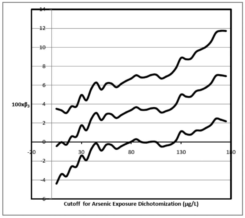
Magnitude of interaction estimates (and 95% confidence interval) for different arsenic concentration dichotomization cutoffs.

5. Conclusions

In this paper we have provided results concerning the conclusions one can draw about causal interactions on the underlying continuous exposure scale when a continuous exposure has been dichotomized. The results extend prior literature on dichotomization from the analysis of main effect to the analysis of interaction. In contrast to a great deal of the existing literature on dichotomization, our results are positive rather than negative. Rather than giving results about the limitations of analysis under dichotomization, our results here demonstrate what one can conclude about underlying continuous exposures even when analysis has been conducted on a dichotomized version of the exposure.

In the results given above we have let the minimum value of the continuous exposure be zero. One could however, restrict the sample to individuals with exposure values above some other minimum (any level below the cutoff h) and apply the results replacing the level zero in the theorems with whatever minimum has been chosen. By considering different dichotomization points of the continuous exposure and also different minimum values of the continuous exposure, one can gain insight on whether the underlying interaction involving the continuous exposure is dose-dependent. Such conclusions may generate useful public health information on how reducing the exposure to certain levels may result in large reductions in the outcome due to interaction between exposures. However, such an approach is also subject to severe multiple testing problems. Bonferonni corrections are likely to be highly conservative as the tests for different cutoff will be highly dependent. Future work could consider alternative approaches for inference across ranges of cutoffs.

An interesting feature of the approach taken in our application is that we were able to avoid modeling of the relationship between the outcome and the continuous exposure. The actual outcome “model” was in fact saturated (with an intercept, two main effects and an interaction term) since the two exposures in the model were dichotomous or had been dichotomized. Confounding was addressed through weighting rather than outcome modeling. The outcome model itself thus could not be misspecified, though conclusions could be sensitive to the models for the weights. This ability to avoid misspecification of the outcome model is potentially desirable as conclusions about the presence of interactions can be sensitive to misspecification of the functional relationship between exposure and outcome; misspecification of a main effect of a continuous exposure in an outcome model can lead to erroneous conclusions about interactions; further discussion of issues of misspecification in the context of interaction analyses are given elsewhere (Vansteelandt et al., 2008; Maity et al., 2009; VanderWeele et al., 2010). This feature of being able to avoid misspecification of the outcome model in interaction analyses is a potential argument in favor of dichotomization. Of course, the price one pays for such dichotomization is somewhat less precise conclusions, as discussed in the paragraph below.

The results we have described here are subject to a number of limitations. First, the results we have provided for drawing inference about causal interaction with regard to the underlying continuous scale give sufficient, but not necessary conditions, for the presence of causal interaction. If conditions (1) and (2) in Theorems 1 and 2 are not satisfied we cannot conclude the absence of causal interaction. Second, when the conditions are satisfied all we can conclude is the presence of a causal interaction which involves some level of the continuous exposure above the cutoff for dichotomization; we cannot say precisely what level or levels of the continuous exposure manifest such causal interaction. Third, the results required reasonable strong assumptions; they required monotonicity assumptions for one of both exposures; even Theorem 1 which tests the stronger of the two probability contrast conditions required a monotonicity assumption for the continuous exposure (though not for the binary exposure). Theorem 2 required a conditional independence assumption; and Theorem 1 gave stronger conclusions with the conditional independence assumption than without. The theorems also required that control had been made for some set of covariates that would suffice to control for confounding of the effects of the exposures on the outcome. This is a fairly standard assumption in causal inference but one which may be violated and, with observational data, will generally at best hold approximately. Future work could consider sensitivity analyses techniques for assessing the sensitivity of one's conclusions about interaction to potential unmeasured confounding.

Future research might also extend the current results in two further directions. First, future research might consider cases in which both exposures are continuous and have been dichotomized and whether analogous results hold in this setting. Second, one might also attempt to develop more general results in which a continuous exposure has not been dichotomized but rather broken up into some number k categories and consider whether conclusions about causal interactions could be drawn on the underlying continuous scale.

Appendix

Proof of Theorem 1

Let Suppose for binary exposure X₁ and dichotomized exposure X₂ = 1(V > h), inequality (1) is satisfied then

$$\begin{array}{l}0<p_{11\mathbf{\text{c}}}-p_{10\mathbf{\text{c}}}-p_{01\mathbf{\text{c}}}\\ =P(D\mid X_1=1,V>h,\mathbf{\text{c}})-P(D\mid X_1=1,V\le h,\mathbf{\text{c}})-P(D\mid X_1=0,V>h,\mathbf{\text{c}})\\ =P(D\mid X_1=1,V>h,\mathbf{\text{c}})-{\int }_{v\le h}P(D\mid X_1=1,V=v,\mathbf{\text{c}})p(v\mid X_1=1,V\le h,\mathbf{\text{c}})dv-{\int }_{v>h}P(D\mid X_1=0,V=v,\mathbf{\text{c}})p(v\mid X_1=0,V>h,\mathbf{\text{c}})dv\\ =P(D\mid X_1=1,V>h,\mathbf{\text{c}})-{\int }_{v\le h}P(D_{1v}\mid X_1=1,V=v,\mathbf{\text{c}})p(v\mid X_1=1,V\le h,\mathbf{\text{c}})dv-{\int }_{v>h}P(D_{0v}\mid X_1=0,V=v,\mathbf{\text{c}})p(v\mid X_1=0,V>h,\mathbf{\text{c}})dv\\ \le P(D\mid X_1=1,V>h,\mathbf{\text{c}})-{\int }_{v\le h}P(D_{10}\mid X_1=1,V=v,\mathbf{\text{c}})p(v\mid X_1=1,V\le h,\mathbf{\text{c}})dv-{\int }_{v>h}P(D_{0h}\mid X_1=0,V=v,\mathbf{\text{c}})p(v\mid X_1=0,V>h,\mathbf{\text{c}})dv\\ =P(D\mid X_1=1,V>h,\mathbf{\text{c}})-{\int }_{v\le h}P(D_{10}\mid \mathbf{\text{c}})p(v\mid X_1=1,V\le h,\mathbf{\text{c}})dv-{\int }_{v>h}P(D_{0h}\mid \mathbf{\text{c}})p(v\mid X_1=0,V>h,\mathbf{\text{c}})dv\\ =P(D\mid X_1=1,V>h,\mathbf{\text{c}})-P(D_{10}\mid \mathbf{\text{c}})-P(D_{0h}\mid \mathbf{\text{c}})\\ =P(D\mid X_1=1,V>h,\mathbf{\text{c}})-P(D_{10}\mid X_1=1,V>h,\mathbf{\text{c}})-P(D_{0h}\mid X_1=1,V>h,\mathbf{\text{c}})\\ =P(D-D_{10}-D_{0h}\mid X_1=1,V>h,\mathbf{\text{c}})\end{array}$$

where the third equality following by consistency, the less-than-or-equal-to inequality follows by monotonicity, and the second to last and fourth to last equalities follow by unconfoundedness. If there were no individual ω with X₁(ω) = 1, V(ω) > h, C(ω) = c and D(ω) = 1 but D₁₀(ω) = D_0h(ω) = 0 then we would have that P(D−D₁₀−D_0h∣X₁ = 1, V > h, c) ≤ 0. Thus if p_11c − p_10c − p_01c > 0 then there must be some individual with X₁(ω) = 1, V(ω) > h, C(ω) = c and D(ω) = 1 but D₁₀(ω) = D_0h(ω) = 0.

Suppose now also X₁ and V are independent conditional on C. In the proof above, the term, ∫_v>h P(D∣X₁ = 0, V = v, c)p(v∣X₁ = 0, V > h, c)dv, could be expressed as

$$\begin{array}{l}{\int }_{v>h}P(D_{0v}\mid X_1=0,V=v,\mathbf{\text{c}})p(v\mid X_1=0,V>h,\mathbf{\text{c}})dv\\ ={\int }_{v>h}P(D_{0v}\mid X_1=0,V=v,\mathbf{\text{c}})p(v\mid X_1=1,V>h,\mathbf{\text{c}})dv\\ ={\int }_{v>h}P(D_{0v}\mid X_1=1,V=v,\mathbf{\text{c}})p(v\mid X_1=1,V>h,\mathbf{\text{c}})dv\\ =P(D_{0v}\mid X_1=1,V=v,\mathbf{\text{c}})\end{array}$$

and we would thus have that 0 < p_11c − p_10c − p_01c implies 0 < P(D − D₁₀ − D_0v∣X₁ = 1, V > h, c) from which it would follow that if p_11c − p_10c − p_01c > 0 then there must be some individual with X₁(ω) = 1, V(ω) > h, C(ω) = c and D(ω) = 1 but D₁₀(ω) = D_0v(ω) = 0.

Addendum to Proof of Theorem 1

Note that if there are a sufficient number of subjects with the minimal level of the exposure, V = 0, instead of testing p_11c−p_10c−p_01c > 0 i.e. p_11c − P(D∣X₁ = 1, V ≤ h, c) − p_01c > 0, one could alternatively test p_11c − P(D∣X₁ = 1, V = 0, c) − p_01c > 0. This second term can be rewritten as P(D∣X₁ = 1, V = 0, c) = P(D₁₀∣X₁ = 1, V = 0, c) = P(D₁₀∣X₁ = 1, V > h, c). Thus the proof of Theorem 1 and the conclusion of Theorem 1 that there must be some individual with X₁(ω) = 1, V(ω) > h, C(ω) = c and D(ω) = 1 but D₁₀(ω) = D_0v(ω) = 0 would apply (without the conditional independence assumption) if p_11c − P(D∣X₁ = 1, V = 0, c) − p_01c > 0 is satisfied rather than p_11c − p_10c − p_01c > 0. The latter condition implies the former since by monotonicity of V, P(D∣X₁ = 1, V = 0, c) ≤ P(D∣X₁ = 1, V ≤ h, c) but estimates of P(D∣X₁ = 1, V = 0, c) may in practice be imprecise if there are few subjects with V = 0 in which case testing p_11c − p_10c − p_01c > 0 may be more practical.

Proof of Theorem 2

We have that

$$\begin{array}{l}{p}_{11\mathbf{\text{c}}}-p_{01\mathbf{\text{c}}}-p_{10\mathbf{\text{c}}}+p_{00\mathbf{\text{c}}}\\ =P(D\mid X_1=1,V>h,\mathbf{\text{c}})-P(D\mid X_1=1,V\le h,\mathbf{\text{c}})-P(D\mid X_1=0,V>h,\mathbf{\text{c}})+P(D\mid X_1=0,V\le h,\mathbf{\text{c}})\\ ={\int }_{v>h}P(D\mid X_1=1,V=v,\mathbf{\text{c}})p(v\mid X_1=1,V>h,\mathbf{\text{c}})dv-{\int }_{v>h}P(D\mid X_1=0,V=v,\mathbf{\text{c}})p(v\mid X_1=0,V>h,\mathbf{\text{c}})dv-{\int }_{v\le h}P(D\mid X_1=1,V=v,\mathbf{\text{c}})p(v\mid X_1=1,V\le h,\mathbf{\text{c}})dv+{\int }_{v\le h}P(D\mid X_1=0,V=v,\mathbf{\text{c}})p(v\mid X_1=0,V\le h,\mathbf{\text{c}})dv\\ ={\int }_{v>h}P(D_{1v}\mid X_1=1,V=v,\mathbf{\text{c}})p(v\mid V>h,\mathbf{\text{c}})dv-{\int }_{v>h}P(D_{0v}\mid X_1=0,V=v,\mathbf{\text{c}})p(v\mid V>h,\mathbf{\text{c}})dv-{\int }_{v\le h}P(D_{1v}\mid X_1=1,V=v,\mathbf{\text{c}})p(v\mid V\le h,\mathbf{\text{c}})dv+{\int }_{v\le h}P(D_{0v}\mid X_1=0,V=v,\mathbf{\text{c}})p(v\mid V\le h,\mathbf{\text{c}})dv\\ ={\int }_{v>h}P(D_{1v}-D_{0v}\mid \mathbf{\text{c}})p(v\mid V>h,\mathbf{\text{c}})dv-{\int }_{v\le h}P(D_{1v}-D_{0v}\mid \mathbf{\text{c}})p(v\mid V\le h,\mathbf{\text{c}})dv\end{array}$$ (A1)

where the third equality follows by consistency and the fourth by unconfoundedness. For the first term in (A1) we have that

$$\begin{array}{l}{\int }_{v>h}P(D_{1v}-D_{0v}\mid \mathbf{\text{c}})p(v\mid V>h,\mathbf{\text{c}})dv\\ ={\int }_{v>h}P(D_{1v}-D_{0v}\mid D_{0v}=1,\mathbf{\text{c}})P(D_{0v}=1\mid \mathbf{\text{c}})p(v\mid V>h,\mathbf{\text{c}})dv+{\int }_{v>h}P(D_{1v}-D_{0v}\mid D_{0v}=0,\mathbf{\text{c}})P(D_{0v}=0\mid \mathbf{\text{c}})p(v\mid V>h,\mathbf{\text{c}})dv\\ =0+{\int }_{v>h}P(D_{1v}\mid D_{0v}=0,\mathbf{\text{c}})P(D_{0v}=0\mid \mathbf{\text{c}})p(v\mid V>h,\mathbf{\text{c}})dv\end{array}$$

where the third equality follows by monotonicity. For the second term in (A1) we have

$$\begin{array}{l}-{\int }_{v\le h}P(D_{1v}-D_{0v}\mid \mathbf{\text{c}})p(v\mid V\le h,\mathbf{\text{c}})dv\\ =-{\int }_{s\le h}P(D_{1s}-D_{0s}\mid \mathbf{\text{c}})p_{V\mid V\le h,\mathbf{\text{c}}}(s)ds\\ =-{\int }_{s\le h}[{\int }_{v>h}\{P(D_{1s}-D_{0s}\mid D_{0v}=1,\mathbf{\text{c}})P(D_{0v}=1\mid \mathbf{\text{c}})+P(D_{1s}-D_{0s}\mid D_{0v}=0,\mathbf{\text{c}})P(D_{0v}=0\mid \mathbf{\text{c}})\}\times P(v\mid V>h,\mathbf{\text{c}})dv]p_{V\mid V\le h,\mathbf{\text{c}}}(s)ds\\ =-{\int }_{s\le h}\{{\int }_{v>h}P(D_{1s}-D_{0s}\mid D_{0v}=1,\mathbf{\text{c}})P(D_{0v}=1\mid \mathbf{\text{c}})+P_V(v\mid V>h,\mathbf{\text{c}})dv\}{p}_{V\mid V\le h,\mathbf{\text{c}}}(s)ds-{\int }_{s\le h}\{{\int }_{v>h}P(D_{1s}\mid D_{0v}=0,\mathbf{\text{c}})P(D_{0v}=0\mid \mathbf{\text{c}})P_V(v\mid V>h,\mathbf{\text{c}})dv\}{p}_{V\mid V\le h,\mathbf{\text{c}}}(s)ds\\ \le 0-{\int }_{s\le h}\{{\int }_{v>h}P(D_{10}\mid D_{0v}=0,\mathbf{\text{c}})P(D_{0v}=0\mid \mathbf{\text{c}})+P_V(v\mid V>h,\mathbf{\text{c}})dv\}{p}_{V\mid V\le h,\mathbf{\text{c}}}(s)ds\\ ={\int }_{v>h}P(D_{10}\mid D_{0v}=0,\mathbf{\text{c}})P(D_{0v}=0\mid \mathbf{\text{c}})P_V(v\mid V>h,\mathbf{\text{c}})dv\end{array}$$

where the third equality and also the inequality both follow by monotonicity. Thus the expression in (A1) is equal to

$${\int }_{v>h}E(D_{1v}-D_{10}\mid D_{0v}=0,\mathbf{\text{c}})P(D_{0v}=0\mid \mathbf{\text{c}})p(v\mid V>h,\mathbf{\text{c}})dv.$$

Suppose that for all v > h there is no individual for whom D_1v(ω) = 1 but D₁₀(ω) = D_0v(ω) = 0 then amongst those with D_0v = 0 we would have that D_1v(ω) = 1 implies D₁₀(ω) = 1 and thus we would have that

$${\int }_{v>h}E(D_{1v}-D_{10}\mid D_{0v}=0,\mathbf{\text{c}})P(D_{0v}=0\mid \mathbf{\text{c}})p(v\mid V>h,\mathbf{\text{c}})dv\le 0.$$

Consequently, if p_11c − p_01c − p_10c + p_00c > 0 then there must be some v > h and some individual ω such that D_1v(ω) = 1 but D₁₀(ω) = D_0v(ω) = 0.

References

- Ahsan H, Chen Y, Parvez F, Argos M, Hussain AI, Momotaj H, Levy D, van Geen A, Howe G, Graziano J. Health Effects of Arsenic Longitudinal Study (HEALS): description of a multidisciplinary epidemiologic investigation. J Expo Sci Environ Epidemiology. 2006;16:191–205. doi: 10.1038/sj.jea.7500449. [DOI] [PubMed] [Google Scholar]
- Assmann SF, Hosmer DW, Lemeshow S, Mundt KA. confidence intervals for measures of interaction. Epidemiology. 1996;7:286–90. doi: 10.1097/00001648-199605000-00012. [DOI] [PubMed] [Google Scholar]
- Chen CL, Hsu LI, Chiou HY, Hsueh YM, Chen SY, Wu MM, et al. Ingested arsenic, cigarette smoking, and lung cancer risk: a follow-up study in arseniasis-endemic areas in Taiwan. JAMA. 2004;292:2984–90. doi: 10.1001/jama.292.24.2984. [DOI] [PubMed] [Google Scholar]
- Chen Y, Graziano JH, Parvez F, Hussain I, Momotaj H, van Geen A, Howe GR, Ahsan H. Modification of risk of arsenic-induced skin lesions by sunlight exposure, smoking, and occupational exposures in Bangladesh. Epidemiology. 2006;17:459–467. doi: 10.1097/01.ede.0000220554.50837.7f. [DOI] [PubMed] [Google Scholar]
- Cohen J. The cost of dichotomization. Applied Psychological Measurement. 1983;7:249–253. [Google Scholar]
- Cole SR, Hernán MA. Constructing inverse probability weights for marginal structural models. American Journal of Epidemiology. 2008;168:656–664. doi: 10.1093/aje/kwn164. [DOI] [PMC free article] [PubMed] [Google Scholar]
- Cox DR. Note on grouping. Journal of the American Statistical Association. 1957;52:543–547. [Google Scholar]
- Delpizzo V, Borghes JL. Exposure measurement errors, risk estimate and statistical power in case-control studies using dichotomous analysis of a continuous exposure variable. International Journal of Epidemiology. 1995;24:851–862. doi: 10.1093/ije/24.4.851. [DOI] [PubMed] [Google Scholar]
- Federov V, Mannino F, Zhang R. Consequences of dichotomization. Pharmaceutical Statistics. 2009;8:50–61. doi: 10.1002/pst.331. [DOI] [PubMed] [Google Scholar]
- Ferreccio C, Gonzalez C, Milosavjlevic V, Marshall G, Sancha AM, Smith AH. Lung cancer and arsenic concentrations in drinking water in Chile. Epidemiology. 2000;11:673–9. doi: 10.1097/00001648-200011000-00010. [DOI] [PubMed] [Google Scholar]
- Gamble MV, Liu X, Ahsan H, Pilsner R, Ilievski V, Slavkovich V, et al. Folate, homocysteine, and arsenic metabolism in arsenic-exposed individuals in bangladesh. Environ Health Perspect. 2005;113:1683–8. doi: 10.1289/ehp.8084. [DOI] [PMC free article] [PubMed] [Google Scholar]
- Gustafson P, Nhu DL. Comparing the effects of continuous and discrete covariate mismeasurement, with emphasis on the dichotomization of mismeasured predictors. Biometrics. 2002;58:878–887. doi: 10.1111/j.0006-341x.2002.00878.x. [DOI] [PubMed] [Google Scholar]
- Hopenhayn-Rich C, Biggs ML, Smith AH, Kalman DA, Moore LE. Methylation study of a population environmentally exposed to arsenic in drinking water. Environ Health Perspect. 1996;104:620–8. doi: 10.1289/ehp.96104620. [DOI] [PMC free article] [PubMed] [Google Scholar]
- Hosmer DW, Lemeshow S. Confidence interval estimation of interaction. Epidemiology. 1992;3:452–56. doi: 10.1097/00001648-199209000-00012. [DOI] [PubMed] [Google Scholar]
- Karagas MR, Tosteson TD, Morris JS, Demidenko E, Mott LA, Heaney J, et al. Incidence of transitional cell carcinoma of the bladder and arsenic exposure in New Hampshire. Cancer Causes Control. 2004;15:465–72. doi: 10.1023/B:CACO.0000036452.55199.a3. [DOI] [PubMed] [Google Scholar]
- MacCallum RC, Zhang S, Preacher KJ, Rucker DD. On the practice of dichotomization of quantitative variables. Psychological Methods. 2002;7:19–40. doi: 10.1037/1082-989x.7.1.19. [DOI] [PubMed] [Google Scholar]
- Maity A, Carroll RJ, Mammen E, Chatterjee N. Testing in semiparametric models with interaction, with applications to gene-environment interactions. Journal of the Royal Statistical Society, Series B. 2009;71:75–96. doi: 10.1111/j.1467-9868.2008.00671.x. [DOI] [PMC free article] [PubMed] [Google Scholar]
- Neyman J. Sur les applications de la thar des probabilities aux experiences Agaricales: Essay des principle. In: Dabrowska D, Speed T, translators. Statistical Science. Vol. 5. 1923. pp. 463–472. Excerpts reprinted (1990) in English. [Google Scholar]
- Robins JM. A new approach to causal inference in mortality studies with sustained exposure period - application to control of the healthy worker survivor effect. Mathematical Modelling. 1986;7:1393–1512. [Google Scholar]
- Robins JM, Hernán MA, Brumback B. Marginal structural models and causal inference in epidemiology. Epidemiology. 2000;11:550–560. doi: 10.1097/00001648-200009000-00011. [DOI] [PubMed] [Google Scholar]
- Rothman KJ. Causes. American Journal of Epidemiology. 1976;104:587–592. doi: 10.1093/oxfordjournals.aje.a112335. [DOI] [PubMed] [Google Scholar]
- Rothman KJ, Greenland S, Lash TL. Modern Epidemiology. 3rd. Philadelphia: Lippincott Williams and Wilkins; 2008. [Google Scholar]
- Royston P, Altman DG, Sauerbrei S. Dichotomizing continuous predictors in multiple regression: a bad idea. Statistics in Medicine. 2006;25:127–141. doi: 10.1002/sim.2331. [DOI] [PubMed] [Google Scholar]
- Rubin D. Estimating causal effects of treatments in randomized and non-randomized studies. Journal of Educational Psychology. 1974;66:688–701. [Google Scholar]
- Senn S. Disappointing dichotomies. Pharmaceutical Statistics. 2003;2:239–240. [Google Scholar]
- Steinmaus C, Yuan Y, Bates MN, Smith AH. Case-control study of bladder cancer and drinking water arsenic in the western United States. Am J Epidemiol. 2003;158:1193–201. doi: 10.1093/aje/kwg281. [DOI] [PubMed] [Google Scholar]
- VanderWeele TJ. Concerning the consistency assumption in causal inference. Epidemiology. 2009a;20:881–883. doi: 10.1097/EDE.0b013e3181bd5638. [DOI] [PubMed] [Google Scholar]
- VanderWeele TJ. Sufficient cause interactions and statistical interactions. Epidemiology. 2009b;20:6–13. doi: 10.1097/EDE.0b013e31818f69e7. [DOI] [PubMed] [Google Scholar]
- VanderWeele TJ, Robins JM. The identification of synergism in the sufficient-component cause framework. Epidemiology. 2007;18:329–339. doi: 10.1097/01.ede.0000260218.66432.88. [DOI] [PubMed] [Google Scholar]
- VanderWeele TJ, Robins JM. Empirical and counterfactual conditions for sufficient cause interactions. Biometrika. 2008;95:49–61. [Google Scholar]
- VanderWeele TJ, Vansteelandt S, Robins JM. Marginal structural models for sufficient cause interactions. American Journal of Epidemiology. 2010;171:506–514. doi: 10.1093/aje/kwp396. [DOI] [PMC free article] [PubMed] [Google Scholar]
- Vansteelandt S, VanderWeele TJ, Tchetgen EJ, Robins JM. Multiply robust inference for statistical interactions. Journal of the American Statistical Association. 2008;103:1693–1704. doi: 10.1198/016214508000001084. [DOI] [PMC free article] [PubMed] [Google Scholar]
- Weinberg CR. How bad is categorization? Epidemiology. 1995;6:345–347. [PubMed] [Google Scholar]