Mathematical model of the dynamics of psychotherapy

Abstract

The success of psychotherapy depends on the nature of the therapeutic relationship between a therapist and a client. We use dynamical systems theory to model the dynamics of the emotional interaction between a therapist and client. We determine how the therapeutic endpoint and the dynamics of getting there depend on the parameters of the model. Previously Gottman et al. used a very similar approach (physical-sciences paradigm) for modeling and making predictions about husband–wife relationships. Given that this novel approach shed light on the dyadic interaction between couples, we have applied it to the study of the relationship between therapist and client. The results of our computations provide a new perspective on the therapeutic relationship and a number of useful insights. Our goal is to create a model that is capable of making solid predictions about the dynamics of psychotherapy with the ultimate intention of using it to better train therapists.

Introduction

One in four adults in the United States suffers with a diagnosable mental disorder. These disorders are the leading cause of disabilities and extract a physical and emotional toll on these individuals, their families, and their communities. Psychotherapy has been shown to be an effective method for treating these disorders (Lambert and Barley 2002; Kazdin 2008; Mozdzierz et al. 2009). Yet, only one quarter of those with these disorders seek psychotherapy and one half drop out after the first session (Muran et al. 2009). A therapist in possession of a better understanding of psychotherapy would be able to improve the success of therapy, reduce the client drop out rate, and yield better ways to train novice therapists.

The success of psychotherapy depends on the nature of the therapeutic relationship between a therapist and a client. Studies have sought to identify the most essential elements of this relationship. Although, those elements are not fully understood, previous psychotherapy studies have reported that the essential element is the personal relationship between the therapist and client, rather than an abstract theoretical framework used by the therapist (Lambert and Barley 2002; Kazdin 2008; Mozdzierz et al. 2009; Muran et al. 2009; Orlinsky and Howard 1977; Martin et al. 2000). This suggests that some features of this relationship can be represented by a model that describes how two people, a dyad, react to themselves and to each other.

Previous studies of this relationship dyad have used the social science paradigm of determining the functional correlations between dependent and independent variables. Here we use a physical science paradigm to investigate the nature of this relationship. Just such a physical science paradigm approach, based on rigorous mathematical modeling, was pioneered by Gottman et al. (2002) to study the interactions between husbands and wives and it proved useful in understanding the stability (or instability) of their marriages. They showed that this approach gives insights into the dynamics of a marriage and has the power to make specific successful predictions about whether the marriage is stable or ends in divorce. We now modify and extend their approach of husband–wife dyads to analyze and understand the therapist–client dyad.

Our work is the first mathematically rigorous model used in the study psychotherapy (with the exception of Gottman’s work, mentioned above). Psychotherapy studies have been done on a ‘case study’ basis or have used an intuitive approach with no mathematical backbone. In our approach, we formulate a rigorous mathematical model of the therapist–client relationship based on published empirical data and our own experience, determine the dynamical properties of that model, and then compare those properties to the known properties of the therapist–client relationship. We will show that this approach yields new insights into the therapeutic relationship. This model cannot, and is not intended to, represent the full nature of the complex human interaction in psychotherapy. However, the fact that it does reveal important insights suggests that some simple dynamical features may underlie the more complex behaviors that emerge in the therapeutic relationship.

The long term goal is for such a theoretical mathematical model to be used to describe and predict successful and unsuccessful therapeutic relationships depending on the parameters or conditions of the relationship. Thus, modeling the therapeutic relationship between therapists and clients may allow researchers to be able to evaluate the quality of the relationship and the effectiveness of specific interventions that might create some significant therapeutic gains with a predictability that has not yet been seen in the clinical research literature. The information may allow researchers to see how specific intervention strategies can predict changes in clients as well as see how specific intervention strategies actually produce changes in clients.

One of the fundamentally novel aspects of our type of approach (beyond the presence of math) is the perspective from which the model is developed. Rather than dissecting the individual components of a system (the client and therapist) in order to study them independently (i.e. compiling an exhaustive survey of possible attributes), we focus on reproducing the emergent dynamics of the relationship that exists between the components. We look for the set of (relevant) properties of the components that play a dominant role in these relationships. It is the relationships that inform the descriptions and properties of the components, not the other way around.

Mathematically, our model is based on coupled, ordinary, nonlinear differential equations. Differential equations have previously been used to model interaction at many scales, from human relationships [e.g. a love affair (Strogatz 1988, 1994)] to functional neurodynamics [e.g. neuronal populations (Ghosh et al. 2008)]. Our perspective shares some commonalities with agent-based modeling, where a system of agents, each following a set of (relatively simple) rules, can give rise to emergent dynamics. Agent-based modeling has been successful in reproducing emergent behaviors in large biological systems [e.g. bird flocking (Reynolds 1987), the spread of epidemics/dynamics of populations (Chowell et al. 2003)], social systems [e.g. conflict (Cederman 2003), ethnic violence (Lim et al. 2007)], and learning [e.g. the impact of emotion on the strength of beliefs (Memon and Treur 2010)]. The advantage of our dynamical systems approach using ordinary differential equations is that we can analyze many of the properties of our system analytically. Our model is therefore much less computationally intensive than most agent-based simulations.

Model

Our mathematical model is a system of two-dimensional, ordinary differential equations (ODEs) representing the emotional valance of a therapist and client. Our ODEs were based on Gottman et al.’s difference equations (Gottman et al. 2002) as reformulated by Larry Liebovitch into differential equations (Liebovitch et al. 2008). We have used a similar approach in models of conflict (Liebovitch et al. 2008) and gene regulatory networks (Liebovitch et al. 2009). The equations for and are

1

2

These equations correspond to the dynamics of the therapist, T (Eq. 1), and client, C (Eq. 2), respectively, where these variables are the emotional valence, or affect, of the therapist and client. For example, a positive value of T would indicate the therapist is in a positive state, and a negative value of T indicates the therapist is in a negative state and similarly for the positive and negative values of C for the client. The variables m ₁ and m ₂ represent the therapist’s and client’s (respectively) inertia to change and b ₁ and b ₂ represent their emotional values when alone. The parameters c ₁ and c ₂ are the coupling/reactivity strengths, or scaling factors, of the influence functions. We assume c _1,2 > 0. The system is coupled via the influence functions F _C(C) and F _T(T).

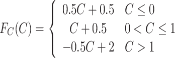
One of the major contributions of this model is the formulation of these influence functions. These are the blueprints for one actor’s emotional affect in response to the other actor’s. Specifically, the influence that the client has on the therapist F _C(C) and the influence that the therapist has on the client F _T(T). These functions are piecewise linear segments in the differential equations reflecting the dynamics of the therapist–client interaction. In other words, they dictate how the two members of the dyad will influence each other. Although these influence functions are based on published empirical data and our own experience, they are somewhat speculative in nature but nonetheless can still provide a starting point for this exploratory project. These functions are

3

4

and the rationale for their choice is explored in “Influence functions”.

The dynamics of the system’s behavior can be analyzed by identifying the critical points of the model, which can represent the final steady state values that the dyad reach at the conclusion of therapy. We then investigate for which initial conditions of T and C the client and therapist will reach the stable states. Finally, we will see how the dynamics of their behavior depend on the parameters of the model.

Influence functions

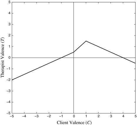
We now describe the influence functions and the empirical basis for their functional form. How the therapist’s valence depends on the client’s valence, F _C(C), is shown in Fig. 1. When the client’s affect is negative, the therapist will exhibit more positive affect, though they may, under prolonged exposure to clients negative affect, begin to exhibit neutral and even negative affect in the face of extreme negative behavior. This may even create a steady state in the negative–negative space, which would effectively be the death of therapy—a “black hole” from which the therapeutic relationship dies (Bohart and Tallman 2010; Gelso 2009; Gelso and Hayes 2002; Horvath and Bedi 2002; Norcross 2010; Safran et al. 2002).

Fig. 1.

F _C(C), Client’s influence function on the therapist

When the client is affectively neutral, therapists will generally utilize strategies to elicit more positive emotions. They will attempt to encourage clients, or try to get the client to focus on their strengths and abilities, in the hopes that this change of focus will change the clients affect (Bohart and Tallman 2010). At the same time, therapists may try to elicit any affect on the part of the client (which may sometimes be negative). However, unless tied to a broader strategy, this is generally born out of frustration and may undermine the therapeutic alliance (Lambert and Barley 2002; Gelso 2009; Horvath and Bedi 2002; Norcross 2010; Safran et al. 2002).

As the client’s affect moves from neutral to positive, initially, the therapist will also exhibit more positive affect. However, there is a point where, as the client’s affect becomes more positive, the therapist may begin to exhibit more neutral affect, as the therapist no longer needs to actively encourage the client, but the positive affect sustains itself (Lambert and Barley 2002; Bohart and Tallman 2010; Gelso 2009; Gelso and Hayes 2002; Horvath and Bedi 2002; Norcross 2010; Safran et al. 2002).

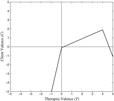
How the client’s valence depends on the therapist’s valence, F _T(T), is shown in Fig. 2. When a therapist exhibits negative affect, the client is likely to react even more negatively. The client may experience therapist negative emotion as judgmental, or a signal of some disappointment in the client. This may be the result of therapist frustration with either the pace of treatment, the client’s unwillingness to change, or fears about the therapist’s own performance in conducting therapy (Bohart and Tallman 2010; Anderson et al. 2010). It is reasonable to suspect that this would be a part of a novice therapist’s practice, but could also be reflective of therapists who may be on the brink of burnout. This frustration may not even be acknowledged by the therapist, but it may get picked up by the client, and move the therapy towards the more negative end of the graph. This is an indicator of a therapeutic rupture, which in turn is a predictor of premature termination from therapy (Muran et al. 2009; Norcross 2010). At the same time, there may be circumstances when a display of negative emotion may be beneficial to the therapeutic relationship. In particular, appropriate confrontation or expressions of disappointment may be necessary feedback to the client. Again, the immediate result may be a therapeutic rupture, but if it is done purposefully or strategically, it may have a long term benefit for the client. The success of this strategy depends a lot on the skill of the therapist and the strength of the therapeutic relationship (Lambert and Barley 2002; Gelso 2009; Gelso and Hayes 2002; Horvath and Bedi 2002; Safran et al. 2002; Anderson et al. 2010; Norcross 2002).

Fig. 2.

F _T(T), Therapist’s influence function on the client

When the therapist is affectively neutral, most clients are likely to be either slightly negative or neutral (particularly early in the therapeutic process). Some clients may not be influenced one way or another to a therapist’s neutral affect, unless they find (i.e., project) it to be a signal of therapist disinterest (e.g., the tabula rasa of psychoanalysis), at which point clients may react negatively (Lambert and Barley 2002; Bohart and Tallman 2010; Gelso 2009; Gelso and Hayes 2002; Horvath and Bedi 2002; Norcross 2010; Safran et al. 2002).

As the therapist’s affect moves from neutral to positive, initially, the client may remain neutral, or slightly negative (Lambert and Barley 2002; Bohart and Tallman 2010; Gelso 2009; Gelso and Hayes 2002; Horvath and Bedi 2002; Safran et al. 2002; Norcross 2002). However, as the therapist’s affect becomes more positive, the client may respond positively by exhibiting more neutral affect (Safran et al. 2002; Skovholt and Jennings 2004). This could be a sign of the client either buying into the therapists message, or a sign that the client is beginning to experience some positive results from the therapeutic intervention. A positive steady state may emerge at this point, where therapeutic gains may be maximized (Norcross 2010). However, as a consequence of extreme expressions of positive affect on the part of the therapist, the client might turn negative (i.e., get turned off, especially if they perceive that it is disingenuous or too pollyannish).

Analysis and solution

To truly appreciate the insights that the model provides, one should look to the phase portraits that emerge from numerically integrating the system from various initial conditions. A phase portrait shows the directions and paths of emotional change for the dyad. These changes are a function of the dyad’s previous emotional state and the parameters of the model. Phase portraits produced by the model are explored in “Phase portraits”.

For the purposes of simplifying the model as much as possible while still preserving the dynamics, let us assume for this numerical analysis a system with parameters m ₁, m ₂ = −1, b ₁, b ₂ = 0, and c ₁, c ₂ = 1. It’s important to note that these particular parameter choices are evenly matched. This would be the sign of novice therapist, as an expert therapist might evoke more reactivity from a client than a client evokes in the therapist (e.g. c ₂ > c ₁).

It is also important at this point to understand the significance of a nullcline. The nullclines exist where the rate of change of the emotional valence of the client or therapist equals zero. In order to explore the dynamics of a system, one must start by finding the critical points, or states, in that system. These critical points are found where the nullclines intersect. In other words, the nullclines define the points in the system where the rate of change of the client and therapist both equal zero. With the values of the parameters mentioned above, the nullclines and become

5

and

6

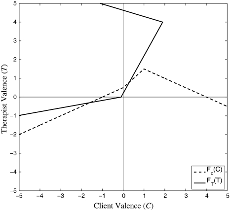
which are shown in Fig. 3. What this means is that for these parameter values, the nullclines equate to the influence functions. The critical points at the intersection of these nullclines are

Fig. 3.

Influence functions, and therefore the nullclines (for the parameter values m _1,2 = −1, b _1,2 = 0 and c _1,2 = 1)

Linear stability analysis is used in order to analyze the dynamics of this system. The stability of each critical point of the model (critical points are defined by the intersection of the nullclines; where the rate of change of both the client’s and therapist’s emotional state equals zero), can be analyzed using it’s corresponding Jacobian matrix. For this system, with these parameters, stability analysis reveals that the first critical point is a saddle (having one positive and one negative eigenvalue) and that the second is an attractor (having two negative eigenvalues). This attractor is the stationary state in the system which defines the values that the variables T and C reach once sufficient time has passed (as long as they are not captured by the unstable force of the saddle point which would result in C and T going to ). The location of this stable state depends on the parameters in the system.

The following equation can be used to generalize the process of stability analysis in the region immediately about a specific critical point.

7

The critical points emerge from the system as a result of the parameter (and influence function) choices. They are best visualized with a phase portrait, which shows the dynamics of the system from various initial conditions. We shall discuss phase portraits in “Phase portraits”.

If we generalize our influence function segments to the form F _C(C) = M ₁ C + B ₁ and F _T(T) = M ₂ T + B ₂, then the segments existing in the region of our critical point we are analyzing can be used to define the slopes I ₁ = c ₁ M ₁ and I ₂ = c ₂ M ₂. In other words, I ₁ and I ₂ are the influence function slopes (M ₁ and M ₂) multiplied by the reactivity scaling factors (c ₁ and c ₂). Once again, this is useful for understanding the dynamics of the relationship in the region immediately surrounding the critical point being analyzed.

The influence functions are defined by fixed numbers (with fixed ranges for the individual segments); therefore it is beyond the scope of this model to have a purely analytical form of these functions (which are treated computationally). In order to approximate a general solution for any given set of intersecting line segments, we must incorporate the parameters that we set to zero in our numerical analysis (b ₁ and b ₂) and the ones we disregarded when doing our stability analysis (B ₁ and B ₂). Let us define β₁ = c ₁ B ₁ + b ₁ and β₂ = c ₂ B ₂ + b ₂. We can then express our system (for any given pair of lines) as

The system has particular solutions

8

and

9

and general solution

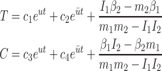where and tr = m ₁ + m ₂ (the trace of the matrix from Eq. 7), det = m ₁ m ₂ − I ₁ I ₂ (the determinant of the matrix from Eq. 7).

Phase portraits

The numerical integration function in Matlab, ODE 113, was used to numerically integrate our system of equations from different initial conditions.

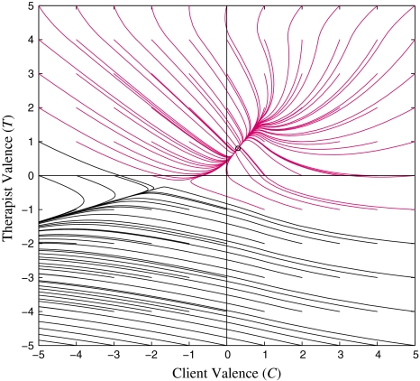
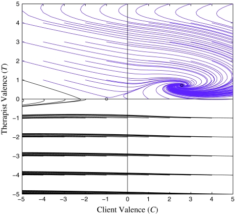
The results of the integration for the parameters defined in “Analysis and solution” are shown in Fig. 4. The trajectories go to the stable attractor at (C, T)₂ = (0.3, 0.8) or are pulled towards and then pushed away from the saddle point at (C, T)₁ = (−1.6, −0.3). The evolution of the system to the stable point would represent a successful therapeutic endpoint. For example, if the client or therapist are initially maximally positive (we’ve all encountered people in this state from time to time), they both end up mildly positive, which is the desired outcome.

Fig. 4.

Phase portrait of the system integrated with parameter values m _1,2 = −1, b _1,2 = 0 and c _1,2 = 1

In Fig. 4, where client and therapist have equal influence with each other, the relationship will likely end up at the positive attractor, as long as the therapist begins with positive emotion. However, if the client starts therapy in a very negative emotional state (C = −5 or −4) then the therapist must be more positive in order to overcome the movement towards the negative saddle point and into the “black hole”. Furthermore, with these parameters of the model, if the client begins therapy with a mild negative state (C = −1) or is neutral, the therapist can also match the negative emotion and still attract the relationship towards the positive stable steady state (approximately T = 1 and C = 1). In addition, if the client starts therapy with very positive affect (C = 2 to 5) the therapist can also display some negative or neutral emotion and still draw the relationship to the positive steady state. Going negative can be a strategy for the therapist to either bring a client who is mildly negative or neutral (C = −1 or 0) about therapy into a positive space. It may also be a strategic method for tamping down a client who is displaying highly (and possibly unrealistically) positive emotions. Since, in this scenario, both the client and the therapist are equally influential of the other, one can look at the other side of the coin. Specifically, if the therapist initially is highly positive (T = 5 to 2) and the client is either negative or positive, the therapist will be drawn down toward the positive stable steady state. The key, it seems, for this relationship to be successful, is that (in most instances) the therapist must avoid beginning with a negative affect. The only exception is if the client is initially very negative, in which case, the relationship will be pulled towards negative emotional states, no matter what the therapist does.

Now, let’s explore what happens as we vary a parameter of our model. We will say that the client is more reactive than the therapist, meaning the client responds strongly to the therapist (c ₁ = 1, c ₂ = 10), which could be the mark of a skilled practitioner.

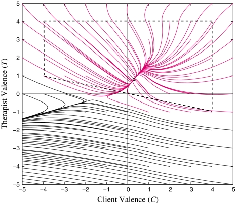
Figure 5 shows the phase-space plots of the trajectories of the therapist and client if the client responds very strongly to the therapist (c ₂ = 10 rather than 1). This may be an indication of a very influential or skilled therapist. Just as in the first phase portrait (Fig. 4), there are two critical points, one of which is a stable steady state attractor where the client is very positive and the therapist is moderately positive, and the other is a saddle point.

Fig. 5.

Phase portrait of the system integrated with parameter values m _1,2 = −1, b _1,2 = 0, c ₁ = 1 and c ₂ = 10

There are some noteworthy results. The therapeutic relationship is attracted toward the positive critical point (steady state attractor) and the emotional state of the relationship spirals, or oscillates up and down in time, before reaching this final steady state. This seems to be in line with clients’ frequent oscillations (i.e. ambivalence) regarding change.

The client winds up more positive than the therapist, and the relationship is attracted to the steady state rapidly (as indicated by the tight spiraling). This seems to be a very good outcome for therapy. There is also a cautionary finding here that the client will likely respond very strongly to any negative input from the therapist. As shown in Fig. 5, any time that the therapist starts with a negative affect on the therapist axis, the relationship will be directed towards the saddle point and from there to increasingly negative values. When the therapist starts with positive affect, the relationship will be directed towards the positive steady state. The only exception to this is when the client affect starts very negative (T = −5 to −3) and the initial therapist affect is only neutral or slightly positive (T = 0 to 1). Thus, just as in Fig. 4, as long as the therapist begins with positive emotion, the client will reach this positive outcome, unless the client starts very negative about treatment.

This model may be an ideal scenario for a brief therapy, where change is swift (as indicated by the tight spiraling) and the client is satisfied. Just as in Fig. 4, as long as the therapist begins with positive emotion, the client will reach this positive outcome, unless the client starts very negative about treatment.

Discussion

Relevant parameters

The dynamics of our system at any given critical point can be determined by Eq. 7.

If m ₁ m ₂ is positive (as is the case if m ₁ = m ₂ = −1), and if I ₁ and I ₂ have opposite signs, the determinant is positive. If I ₁ and I ₂ have the same sign, the sign of the determinant depends on whether the product I ₁ I ₂ is large enough to outweigh the positive influence of the inertial terms. The point here is if I ₁ and I ₂ have the same sign, and are large enough, then det < 0 and we have a saddle.

As stated, the slope I of a nullcline at the intersection point with another nullcline plays a large role in determining the dynamics at that critical point. The inertia of the actor m also has a significant role to play in the dynamics as well. We will now explore the importance of the determinant (det), trace (tr) and discriminant (tr ² − 4det) of the coefficient matrix of the system to analyzing the system’s dynamics at each of the critical points. If the det < 0, we get a saddle point. If the det > 0 and tr ² − 4det > 0, the critical point is a stable point. If tr ² − 4det < 0, then the critical point is a stable spiral. Recall that the coefficient matrix is determined by the parameters of the system and the influence functions (Table 1).

Table 1.

Relevant parameters

Signs of I 1, I 2	Magnitude	Expected behavior
Same	Large	Saddle
Same	Small	Attractor
Opposite	Small	Attractor
Opposite	Large	Spiral

Limit cycles

We now show that for this system, with these influence functions, there is no limit cycle present. The reason a limit cycle is not desirable in this model is simple: a limit cycle would represent a never-ending oscillation of client and therapist emotional state, which would not be a realistic therapeutic outcome.

Utilizing the concept of a trapping domain from Poincare-Bendixson’s theorem, we show that the flow of trajectories along the edges of a closed, appropriately defined region (what is important is the general shape of this region, rather than the specific equations defining it’s boundaries) such as the dashed line shown in Fig. 6 are inwards, towards the stable attractor point. If the flow never leaves the trapping domain, and we have shown that only a stable fixed point exists within this domain, then no limit cycle can exist. This does not preclude the existence of stable spiral behavior within the trapping domain, however.

Fig. 6.

Visualization of the trapping domain (dashed line)

Once a trajectory of the system flows into the trapping domain, it will not escape. The trapping domain is depicted in Fig. 6.

For the attractor point (C, T)₂, which exists at the intersection of the nullclines (Eqs. 5 and 6) derived from Eqs. 3 and 4 (where 0 < C ≤ 1 and 0 < T ≤ 4) at becomes and for our standard parameter values m ₁ =  − 1, b ₁ = 0 and c ₁ = 1, this becomes

10

Likewise, becomes and with the standard parameter values m ₂ =  −1, b ₂ = 0 and c ₂ = 1, this becomes

11

What follows is one of a range of possible domain sizes, but the concepts remain the same.

First, let us define, as generally as possible (without being redundant), our trapping domain’s left boundary. For C = −4 and will always be positive and flow rightwards. To test this, we substitute these values into Eq. 11. The rate of change is positive and the flow is rightwards or inwards toward the stable point.

Next, let us define our trapping domain’s upper boundary. For C = −4 ≤ x ≤ 4 and will always be negative and flow downwards. To test this, we substitute these values into Eq. 10. The rate of change is negative and the flow is downwards or inwards toward the stable point.

Now, let us define our trapping domain’s right boundary. For C = 4 and will always be negative and flow leftwards. To test this, we substitute these values into Eq. 11. The rate of change is negative and the flow is leftwards or inwards toward the stable point.

The trapping domain’s lower boundary is created by the saddle point in the negative–negative space (C, T)₁ = −1.6, −0.3. We shall define this lower boundary by the lower dashed line seen in Fig. 6. It begins at C, T = −4, 1 and ends at C, T = 4, −1. The equation for this line segment is T = −0.25C, where −4 ≤ C ≤ 4. Recall that a saddle point is stable along one direction (attractive) and unstable along the other (repulsive). The unstable region of this saddle point is explicitly defined (as shown in “Analysis and solution”) by our stability analysis and the integration of the system as seen in the phase portrait shown in Fig. 6. Any trajectory entering the trapping domain from this lower boundary will have been pushed in by the unstable force of the saddle point and will be pulled in by the stable attractor. On the other side of this saddle point (the lower left region of Fig. 6), trajectories are pushed into the therapeutic “black hole” from which there is no return.

No limit cycle can exist in this system because any trajectory entering the trapping domain will never escape, and within the trapping domain there only exists a single critical point, which is a stable attractor. Any trajectory not eventually caught by the attractive force of the stable point that resides within the trapping domain will be subject to the unstable force of the saddle point and descend into further negativity.

Bifurcation diagrams

We now present bifurcation diagrams showing how the critical points of the system change when independently changing the inertia, m ₂, of the client and the relative strength of the influences between the therapist and client, α = c ₂/c ₁.

Varying m₂

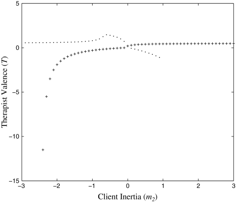
Shown in Fig. 7 are the therapist values for the fixed points as m ₂ is varied from −3 to 3 in steps of 0.1. The other parameters of the model are m ₁ = −1, c _1,2 = 1, b _1,2 = 0. For m ₂ ≤ −2.5, our saddle point ceases to exist. There is also a “hump” created by the shifting stable point from m ₂ = −0.75 to m ₂ = −0.25, with a peak at m ₂ = −0.5. The stable point and saddle exist at the same level of emotional valence for the therapist at m ₂ = 0 and for 0 < m ₂ < 1 the stable point begins to descend into negative emotional space for the therapist. At m ₂ = 1, the stable point ceases to exist and only the saddle remains for increasing values of m ₂.

Fig. 7.

Values of the attractor (.) and saddle (+) points of the therapist as a function of m ₂

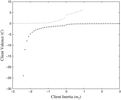
Shown in Fig. 8 are the client values for the fixed points as m ₂ is varied from −3 to 3 in steps of 0.1. The other parameters of the model are m ₁ = −1, c _1,2 = 1, b _1,2 = 0. This bifurcation diagram shows characteristics similar to our therapist plot. Specifically, the critical saddle point ceasing to exist at about m ₂ = −2.5. The stable point also shows signs of the hump at m ₂ = −0.5, but then continues in an upward trend right until the stable point ceases to exist at m ₂ = 1. The saddle point continues to exist for values of m ₂ > −2.5, just as in Fig. 7.

Fig. 8.

Values of the attractor (.) and saddle (+) points of the client as a function of m ₂

It should be kept in mind that the inertia of an actor is thought of as a dampening force on the dynamics of the system (i.e. m ₂ < 0 typically), so m ₂ values greater than zero will be unusual. Another way of interpreting a non negative m ₂ value would be that the therapist is exhibiting such a strong influence on the client, that the client has negative inertia. It appears that the actor with the least inertia (highest value of m ₂) will have the most positive emotional outcome, assuming the initial conditions are such that the trajectory goes to the stable point.

Varying α

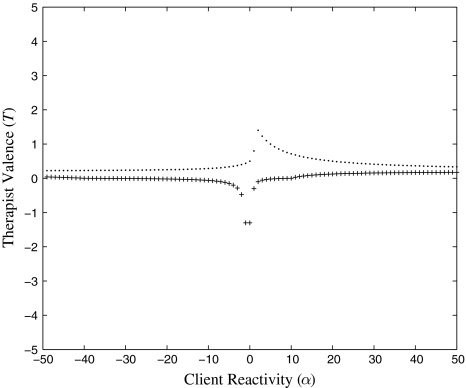
Shown in Fig. 9 are the therapist values for the fixed points as α = c ₂/c ₁ is varied from −50 to 50 in steps of 1, by increasing the client’s coupling strength, c ₂. The parameter c ₁ = 1 and is held constant throughout. The other parameters of the model are m _1,2 = −1, b _1,2 = 0. For α < 0, which would indicate a negative coupling strength on the client side (this is counterintuitive for a human dyad, much as positive values of m are counterintuitive), the stable point remains in slightly positive space for the therapist. A peak in the therapist’s emotional state is seen at around α = 2, which is exactly where the client’s emotional dynamic changes from a steep increase to a more gradual one.

Fig. 9.

Values of the attractor (.) and saddle (+) points of the therapist as a function of α = c ₂/c ₁

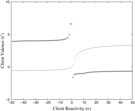
Shown in Fig. 10 are the client values for the fixed points as α is varied from −50 to 50 in steps of 1. The parameter c ₁ = 1 and is held constant throughout. The other parameters of the model are m _1,2 = −1, b _1,2 = 0. When α < 0, we see that the stable attractor exists in the negative space for the client, while the saddle is in positive emotional space. When α > 0 and the client’s reactivity scaling factor is raised, we see that the client’s emotional end state (the stable point) becomes more positive as well. This illustrates the first of our conclusions (below) that the person who is the most responsive ends up being the most positive.

Fig. 10.

Values of the attractor (.) and saddle (+) points of the client as a function of α = c ₂/c ₁

Conclusions

Through determining how the endpoints, stability, and dynamics of the system depends on various parameters, we have drawn a number of conclusions from this theoretical framework.

The therapist or client who is the most responsive to the other ends up being the most positive

If the client is more responsive to the affect of the therapist, the client reaches a more positive affect than the therapist. If the therapist is more responsive to the affect of the client, the therapist reaches a more positive affect than the client. This means that to achieve the most positive state for the client, which defines successful therapy, the therapist’s responses to the client should be moderated. This important conclusion of the model may provide a dynamical basis for understanding the intuitive empirical finding, over the last century of psychotherapy, of the advantages to be gained from the therapist presenting a low reactivity face to the client. In terms of the mathematics of the model, increasing the value of the influence function scaling factor c _1,2 will result in an increase in the slope I _1,2. This raises the respective coordinate along its axis, thus improving the emotional state of the person being influenced.

Recall that our fixed point is defined for T by Eq. 8 and for C by Eq. 9. In order for this conclusion to hold true, the person’s uninfluenced emotional state (their emotional state when alone) must not be negative (β_1,2 ≥ 0).

The final stable state of the client may be approached through emotional ups and downs

For many of the scenarios we’ve studied, the steady state is reached through a spiral trajectory. This translates to the client and therapist each going through up and down emotional swings before reaching their final steady states. These emotional swings are not necessarily backsliding on the part of the client. Rather they are a direct result of the dynamics driven by the therapist and client influence functions, and therefore must be expected in these therapeutic relationships.

A client who is less influenced by their own previous state takes longer to reach their final stable state

A person who is less influenced by their own previous state has a slowed approach to a final steady state attractor. The smaller a person’s inertial term m, the more likely they are to oscillate before reaching their steady state. Complementarily, the lower the magnitude of the trace tr of the system matrix, the slower the spiral decays.

A client who is less influenced by their own previous state follows a similar trajectory to one that is more responsive to their therapist

Responding more weakly to one’s own previous emotional state yields a similar pattern of dynamics as responding more strongly to the other person. We define types of phase portraits by the number and type of critical points that exist.

Suppose a point is close to being a saddle point. The determining factor for that is whether det = m ₁ m ₂ − I ₁ I ₂ < 0. If we’re on the tipping point between being a saddle and an attractor, we can assume that I ₁ and I ₂ have the same sign, so the only question is whether they are big enough. In this case, increasing I ₁ I ₂ will have the same effect as decreasing m ₁ m ₂, that is to say, increasing the influences has the same effect as weakening your response to your previous emotional state.

Now suppose a point is on the brink between being a stable point and a spiral. The determining factor is whether (m ₁ − m ₂)² + 4I ₁ I ₂ < 0. If we’re on the tipping point between being an attractor and a spiral, we can assume that I ₁ and I ₂ have opposite signs. In this case, increasing the influence functions has the same effect as bringing m ₁ and m ₂ closer together.

Summary

As noted above, this model cannot, and is not intended to, represent the full nature of the complex human interaction in psychotherapy. However, the fact that it does reveal important insights about therapist neutrality, client emotional swings, and the reciprocal roles of inertia and influence between therapist and client, are consistent with therapists’ empirical experiences. This may suggest that some simple dynamical features may underlie the more complex behaviors that emerge in the therapeutic relationship.

Future work

The present exploratory work is already quite a significant conceptual leap in trying to develop a new approach that may shed light on the dynamics of psychotherapy. We hope that it will serve as a firm starting point to further develop new theoretical and empirical studies. Theoretically, Gottman et al. (2002) found that changes in the influence functions with time were essential features of how relationships in marriages were improved (or worsened). We want to explore how changing these influence functions, during the course of therapy, can improve the therapeutic outcome. Experimentally, again as Gottman et al. (2002) did, we want to video record psychotherapy sessions, code the time dependent valence of the therapist and client, use that data to determine the best fit parameters of the model system, and then determine which of those parameters best correlates with independent measures of the success of therapy. We are especially interested in learning how the influence functions and dynamics differ between inexperienced and experienced therapists.

The long term goal is to understand enough about the dynamics of psychotherapy to suggest which approaches are likely to be the most beneficial for the client and how those approaches can be empirically tested. This may also lead to new ways to train therapists to utilize those best approaches.

References

- Anderson T, Lunnen KM, Ogles BM. Putting models and techniques in context. In: Duncan BL, Miller SD, Wampold BE, Hubble MA, editors. The heart and soul of change: delivering what works in therapy. 2. Washington, D.C.: American Psychological Association; 2010. [Google Scholar]
- Bohart AC, Tallman K. Clients: the neglected common factor. In: Duncan BL, Miller SD, Wampold BE, Hubble MA, editors. The heart and soul of change: delivering what works in therapy. 2. Washington, D.C.: American Psychological Association; 2010. [Google Scholar]
- Cederman LE. Modeling the size of wars: from billiard balls to sand piles. Am Political Sci Rev. 2003;97(1):135–150. doi: 10.1017/S0003055403000571. [DOI] [Google Scholar]
- Chowell G, Hyman JM, Eubank S, Castillo-Chavez C. Scaling laws for the movement of people between locations in a large city. Phys Rev E. 2003;68:066102. doi: 10.1103/PhysRevE.68.066102. [DOI] [PubMed] [Google Scholar]
- Gelso CJ. The real relationship in a postmodern world: theoretical and empirical explorations. Psychother Res. 2009;19(3):253–264. doi: 10.1080/10503300802389242. [DOI] [PubMed] [Google Scholar]
- Gelso CJ, Hayes JA. The management of countertransferrence. In: Norcross JC, editor. Psychotherapy relationships that work: therapist contributions and responsiveness to patient needs. New York: Oxford University Press; 2002. [Google Scholar]
- Ghosh A, Rho Y, McIntosh AR, Kötter R, Jirsa VK. Cortical network dynamics with time delays reveals functional connectivity in the resting brain. Cogn Neurodyn. 2008;2:115–120. doi: 10.1007/s11571-008-9044-2. [DOI] [PMC free article] [PubMed] [Google Scholar]
- Gottman J, Murray J, Swanson C, Tyson R, Swanson K. The mathematics of marriage: nonlinear models. Cambridge: MIT Press; 2002. [Google Scholar]
- Horvath AO, Bedi RP. The alliance. In: Norcross JC, editor. Psychotherapy relationships that work: therapist contributions and responsiveness to patient needs. New York: Oxford University Press; 2002. [Google Scholar]
- Kazdin AE. Evidence-based treatment and practice: new opportunities to bridge clinical research and practice, enhance the knowledge base, and improve patient care. Am Psychol. 2008;63:146–159. doi: 10.1037/0003-066X.63.3.146. [DOI] [PubMed] [Google Scholar]
- Lambert MJ, Barley DE. Research summary on the therapeutic relationship and psychotherapy outcomes. In: Norcross JC, editor. Psychotherapy relationships that work: therapist contributions and responsiveness to patient needs. New York: Oxford University Press; 2002. [Google Scholar]
- Liebovitch LS, Naudot V, Vallacher R, Nowak A, Bui-Wrzosinska L, Coleman P. Dynamics of two-actor cooperation-competition conflict models. Physica A. 2008;387:6360–6378. doi: 10.1016/j.physa.2008.07.020. [DOI] [Google Scholar]
- Liebovitch LS, Shehadeh LA, Jirsa VK, Hütt M-T, Marr C. Determining the properties of gene regulatory networks from expression data. In: Das S, Caragea D, Welch S, Hsu WH, editors. Handbook of research on computational methodologies in gene regulatory networks. Hershey: IGI Global; 2009. [Google Scholar]
- Lim M, Metzler R, Bar-Yam Y. Global pattern formation and ethnic/cultural violence. Science. 2007;317(5844):1540–1544. doi: 10.1126/science.1142734. [DOI] [PubMed] [Google Scholar]
- Martin DJ, Garske MP, Davis MK. Relation of the therapeutic alliance with outcome and other variables: a meta-analytic review. J Consult Clin Psychol. 2000;68:438–450. doi: 10.1037/0022-006X.68.3.438. [DOI] [PubMed] [Google Scholar]
- Memon ZA, Treur J. On the reciprocal interaction between believing and feeling: an adaptive agent modelling perspective. Cogn Neurodyn. 2010;4:377–394. doi: 10.1007/s11571-010-9136-7. [DOI] [PMC free article] [PubMed] [Google Scholar]
- Mozdzierz G, Peluso PR, Lisiecki J. Principles of counseling and psychotherapy: learning the essential domains and nonlinear thinking of master practitioners. New York: Routledge; 2009. [Google Scholar]
- Muran JC, Gorman BS, Eubanks-Carter C, et al. The relationship of early alliance ruptures and their resolution to process and outcome in three time-limited psychotherapies for personality disorders. Psychother Theory Res. 2009;46(2):233–248. doi: 10.1037/a0016085. [DOI] [PubMed] [Google Scholar]
- Norcross JC. Psychotherapy relationships that work: therapist contributions and responsiveness to patient needs. New York: Oxford University Press; 2002. [Google Scholar]
- Norcross JC. The therapeutic relationship. In: Duncan BL, Miller SD, Wampold BE, Hubble MA, editors. The heart and soul of change: delivering what works in therapy. 2. Washington, D.C.: American Psychological Association; 2010. [Google Scholar]
- Orlinsky DE, Howard KE. The therapist’s experience of psychotherapy. In: Gurman AS, editor. Effective psychotherapy: a handbook of research. New York: Pergamon; 1977. [Google Scholar]
- Reynolds CW. Flocks, herds and schools: a distributed behavioral model. Comput Graph. 1987;21(4):25–34. doi: 10.1145/37402.37406. [DOI] [Google Scholar]
- Safran JD, Muran JC, Samstang LW, Stevens C. Repairing alliance ruptures. In: Norcross JC, editor. Psychotherapy relationships that work: therapist contributions and responsiveness to patient needs. New York: Oxford University Press; 2002. [Google Scholar]
- Skovholt TM, Jennings L. Master therapists: exploring expertise in therapy and counseling. Boston: Allyn & Bacon; 2004. [Google Scholar]
- Strogatz SH. Love affairs and differential equations. Math Mag. 1988;61(1):35. doi: 10.2307/2690328. [DOI] [Google Scholar]
- Strogatz SH. Nonlinear dynamics and chaos: with applications to physics, biology, chemistry, and engineering. Reading: Addison-Wesley; 1994. [Google Scholar]