A Finite Field Method for Calculating Molecular Polarizability Tensors for Arbitrary Multipole Rank

Abstract

A finite field method for calculating spherical tensor molecular polarizability tensors α_lm;l′m′ = ∂Δ_lm/∂ϕ_l′m′* by numerical derivatives of induced molecular multipole Δ_lm with respect to gradients of electrostatic potential ϕ_l′m′* is described for arbitrary multipole ranks l and l′. Inter-conversion formulae for transforming multipole moments and polarizability tensors between spherical and traceless Cartesian tensor conventions are derived. As an example, molecular polarizability tensors up to the hexadecapole-hexadecapole level are calculated for water at the HF, B3LYP, MP2, and CCSD levels. In addition, inter-molecular electrostatic and polarization energies calculated by molecular multipoles and polarizability tensors are compared to ab initio reference values calculated by the Reduced Variation Space (RVS) method for several randomly oriented small molecule dimers separated by a large distance. It is discussed how higher order molecular polarizability tensors can be used as a tool for testing and developing new polarization models for future force fields.

I Introduction

Molecular polarizability tensors have played an important role in our understanding of intermolecular forces. The interaction energy of a molecule in an external electrostatic field is completely described by molecular multipoles and polarizability tensors as shown in the pioneering works of many researchers^1–10. In recent times, molecular polarizability tensors^11–13 are often calculated by finite field methods^14–18, in which the molecular polarizability is expressed as a numerical derivative of induced molecular multipole moment with respect to gradients of external electrostatic potential. For example, the components of the ab initio molecular dipole-dipole polarizability tensor α_pq can be calculated as a derivative of induced molecular dipole moment μ_p with respect to external electric field E_q

$${\alpha }_{pq}=\frac{\partial {\mathbf{\mu }}_p}{\partial {\mathbf{E}}_q}$$ (1)

In addition, Dykstra and co-workers^19–21 have calculated molecular polarizability tensors of higher multipole rank at the Hartree Fock (HF) level using analytic derivative techniques²².

Molecular polarizability tensors have been instrumental in developing polarization models for inter-molecular forces, which for example, have been used in developing polarizable models for water^23–34. Some common polarization models are based on induced dipoles^35–37, Drude oscillators³⁸, fluctuating charges^39–42, and continuum dielectric models^43,44. In many cases, the polarizability parameters are fit to or tested against experimental or theoretical molecular dipole-dipole polarizability tensors. In order to more accurately capture the anisotropy in the response charge density, Stone and co-workers^45–48 have proposed Distributed Polarizabilities, in which the static density susceptibility function^49,50 (also see eqns. 4 and 5) is projected onto an atomic point multipole basis set using Distributed Multipole Analysis^51,52 methods. Recent work^53–57 has focused on investigating new polarization models based on induced atomic dipoles and quadrupoles. The models based on induced higher order atomic multipoles are often tested by calculating molecular dipole-quadrupole and quadrupole-quadrupole molecular polarizability tensors and comparing with reference ab initio values. In addition, molecular polarizability tensors have been used directly as the model for polarization energy for small molecules, such as water. For example, molecular polarizability tensors up to the quadrupole-quadrupole^23–25 or octupole-octupole²⁹ level have been used to construct models of water-water inter-molecular interactions.

As described above, higher order molecular polarizability tensors can be used as a tool for testing and developing new polarization models for inter-molecular energy. However, the calculation of higher order molecular polarizability tensors is not routine. Aside from some notable exceptions discussed below, most quantum chemistry programs only calculate dipole-dipole molecular polarizability tensors. Finite field procedures^14–18 have been described for calculating molecular polarizability tensors up to the quadrupole-quadrupole or dipole-octupole level for highly symmetric small molecules or atoms. In this work, we describe a finite field derivative method for calculating molecular polarizability tensors α_lm;l′m′ of arbitrary multipole ranks l and l′ for molecules of any shape and size. The molecular polarizability tensors are calculated as numerical derivatives of induced multipole moment Δ_lm with respect to gradients of external electrostatic potential ϕ_l′m′*.

As mentioned above, some quantum chemistry programs do calculate higher order molecular polarizability tensors with some caveats. CADPAC⁵⁸ calculates dipole-quadrupole and quadrupole-quadrupole polarizability tensors in the traceless Cartesian convention at the Self Consistent Field (SCF) level. MOLPRO⁵⁹ and DALTON⁶⁰ calculates ‘pure’ Cartesian molecular polarizability tensors for arbitrary multipole rank at various levels of quantum theory, which include both SCF and electron correlation methods (MP2, CCSD, etc). However for modeling purposes, it would be more useful to express the molecular polarizabilities in their traceless Cartesian and spherical tensor conventions. Equations for inter-converting polarizability tensors between traceless Cartesian and spherical tensor conventions have been given for specific cases up to the quadrupole-quadrupole level^7,61. In this work, conversion formulae are derived for transforming multipoles and polarizability tensors between ‘pure’ Cartesian, traceless Cartesian, and spherical tensor conventions for arbitrary multipole rank. The derivations are mainly based on the polynomial properties of the regular solid harmonic functions⁶² C_lm (x, y, z) (see eqn. A.8 of the appendix). For multipoles, similar conversion formulae have been given in previous works^63,64, but not for polarizabilities.

As a test, molecular polarizabilities up to the hexadecapole-hexadecapole level are calculated for water in the equilibrium geometry at the HF, B3LYP, and MP2 levels using the correlation consistent basis sets^65–67. Special attention is focused on the convergence of molecular polarizability tensors with respect to increasing basis set size for various multipole ranks. In addition, molecular polarizability tensors up to the quadrupole-quadrupole level are calculated for water at the CCSD/d-aug-cc-pVQZ level and compared to previous ab initio calculations^21,68–72. Direct comparison to experiment⁷³ would require vibrational-rotational corrections^71,72,74.

An interesting question arises: ‘How important are the higher order molecular polarizability tensors in reproducing long range inter-molecular polarization energies?’ It is well-known that the inter-molecular electrostatic and polarization energies between two molecules separated by a large enough distance can be calculated by applying the molecular multipole approximation to intermolecular perturbation theory^61,75. The long range electrostatic energy can be calculated from the interaction of both molecular multipoles, while the long range polarization energy can be calculated from the interaction of molecular multipoles and polarizability tensors between molecules. Increasing the multipole rank l gives more accurate estimates of electrostatic and polarization energy. However, the effect of increasing the multipole rank l is not often quantified. In this work, inter-molecular electrostatic and polarization energies are calculated by molecular multipoles and polarizability tensors for several randomly oriented small molecule dimers separated by a ‘large distance’. The multipolar electrostatic and polarization energies are compared to ab initio reference values calculated at the HF/6-31++G** level using the Reduced Variation Space (RVS) method^76,77 in GAMESS⁷⁸. The accuracy of the energies calculated by molecular multipoles/polarizabilities is studied as a function of increasing multipole rank. A necessary condition for the multipole approximation between two molecules is that their molecular charge densities do not significantly overlap. It has been shown⁷⁹ that the overlap of inter-molecular charge density is approximately proportional to the inter-molecular exchange-repulsion energy. Therefore, we have constructed randomly oriented dimers separated by a ‘large distance’, in which the inter-molecular exchange-repulsion energy is less than 0.01 kcal/mol (3.5 – 5.0 Å closest atom-atom separation). Although the Hartree Fock (HF) level does not include electron correlation⁸⁰ and the 6-31++G** basis set is much smaller than most of the correlation consistent basis sets, the comparison of electrostatic and polarization energies calculated by molecular multipoles/polarizability tensors with ab initio demonstrates the importance of including higher order multipoles.

A special note concerning the calculation of molecular multipoles should be made. For approximate, non-variational wave-functions Ψ₀ which do not satisfy the Hellman-Feynmann theorem (e.g. MP2 or CCSD), it has been shown^81,82 that the molecular multipole moments calculated by taking the expectation value of the multipole moment operator do not reproduce the correct interaction energy when the molecule is placed in an external electrostatic field. For example, the interaction energy U of a molecule in a uniform weak external electric field E is given by

$$U(\mathbf{E})=-\mathbf{\mu }·\mathbf{E}-\frac{1}{2}\mathbf{E}·\mathbf{\alpha }·\mathbf{E}+\mathrm{..}$$ (2)

where μ is the molecular dipole moment and α is the molecular dipole-dipole polarizability matrix. The ab initio molecular dipole moment can be calculated by differentiating U with respect to E in the limit of small field strength.

$$\mathbf{\mu }={-\frac{\partial U}{\partial \mathbf{E}}|}_{\mathbf{E}=0}$$ (3)

However, if Ψ₀ does not satisfy the Hellman-Feynmann theorem, the definition for μ in eqn. 3 does not agree with its quantum mechanical expectation value μ ≠ 〈Ψ₀ |μ̂| Ψ₀〉. In this case, the recommended definition for molecular dipole is the energy derivative in eqn. 3. In this work, ab initio molecular multipoles are calculated from relaxed densities^83,84 which give the correct electrostatic energy in the presence of external fields.

We have written a program to calculate molecular polarizability tensors up to hexadecapole-hexadecapole using the output files from the Gaussian⁸⁵ suite of quantum chemistry programs and we plan to make our program freely available. In addition, mathematical background information^{61,62,86–90} is summarized in the appendix, while technical details behind some of the derivations are given in the Supplementary Information along with additional results.

II Methods

A. Review of Molecular Multipoles/Polarizability Tensors

The energy U of a molecule in a time-independent electrostatic field ϕ(r) can be expanded in a power series to second order in ϕ(r) by

$$U=U_0+\int d^3\mathbf{r}\rho (\mathbf{r})\varphi (\mathbf{r})+\frac{1}{2}\iint d^3{\mathbf{r}d}^3{\mathbf{r}}^{\prime }\varphi (\mathbf{r})\eta (\mathbf{r},{\mathbf{r}}^{\prime })\varphi ({\mathbf{r}}^{\prime })+\mathrm{..}$$ (4)

where U₀ is the energy of the molecule in vacuum, ρ(r) is the molecular charge density in vacuum, and η(r, r′) is the static density susceptibility function^49,50 defined by functional derivatives⁴⁹ of interaction energy U with respect to electrostatic potential

$$\rho (\mathbf{r})={\frac{\delta U}{\delta \varphi (\mathbf{r})}|}_{\varphi =0}\eta (\mathbf{r},{\mathbf{r}}^{\prime })={\frac{{\delta }^{2}U}{\delta \varphi (\mathbf{r})\delta \varphi ({\mathbf{r}}^{\prime })}|}_{\varphi =0}$$ (5)

If the charge source of the external potential does not overlap with the molecular charge distribution, ∇²ϕ= 0 in the volume encompassing the molecule. In this case, Rowe⁸⁷ has shown that ϕ(r) can be expanded about the molecular center R in a ‘spherical tensor Taylor series’ by

$$\varphi (\mathbf{r})=\sum _{l=0}^{\infty }\sum _{m=-l}^l\frac{C_{lm}(\mathbf{r}-\mathbf{R})C_{lm}^{\ast }(\nabla )}{(2l-1)!!}\varphi (\mathbf{R})$$ (6)

where * indicates the complex conjugate, C_lm(r) is a solid harmonic polynomial⁶² (eqns. A.3 and A.8), and C_lm (∇) is a solid harmonic gradient operator^62,87 (eqn. A.10). The molecular center R is arbitrary. However, the multipole expansion will have faster convergence properties if R corresponds to a central point of the molecule, such as the center of mass or center of nuclear charge. Inserting eqn. 6 into eqn. 4 results in a multipole expansion of the interaction energy U into electrostatic U_ele and polarization U_pol contributions

$$U=U_0+U_{\mathit{ele}}+U_{\mathit{pol}}+\mathrm{..}$$ (7)

$$U_{\mathit{ele}}=\sum _{lm}{Q}_{lm}{\varphi }_{lm}^{\ast }$$ (8)

$$U_{\mathit{pol}}=-\frac{1}{2}\sum _{lm}\sum _{l^{\prime }{m}^{\prime }}{\alpha }_{lm;l^{\prime }{m}^{\prime }}{\varphi }_{lm}^{\ast }{\varphi }_{l^{\prime }{m}^{\prime }}^{\ast }$$ (9)

where Q_lm is the molecular multipole moment in vacuum, α_lm;l′m′ is a molecular polarizability tensor, and ϕ_l′m′* is an external field gradient evaluated at R defined by

$$Q_{lm}\equiv \int d^3\mathbf{r}\rho (\mathbf{r})C_{lm}(\mathbf{r}-\mathbf{R})$$ (10)

$${\alpha }_{lm;l^{\prime }{m}^{\prime }}\equiv -\iint d^3{\mathbf{r}d}^3{\mathbf{r}}^{\prime }\eta (\mathbf{r},{\mathbf{r}}^{\prime })C_{lm}(\mathbf{r}-\mathbf{R})C_{l^{\prime }{m}^{\prime }}({\mathbf{r}}^{\prime }-\mathbf{R})$$ (11)

$${\varphi }_{lm}^{\ast }\equiv \frac{C_{lm}^{\ast }(\nabla )\varphi (\mathbf{R})}{(2l-1)!!}$$ (12)

The energy U in eqn. 7 may be viewed as a function ϕ_l′m′*. The molecular multipole Q_lm and polarizability α_lm;l′m′ can also be calculated as derivatives of energy by

$$Q_{lm}={\frac{\partial U}{\partial {\varphi }_{lm}^{\ast }}|}_{\varphi =0}$$ (13)

$${\alpha }_{lm;l^{\prime }{m}^{\prime }}={-\frac{{\partial }^{2}U}{\partial {\varphi }_{lm}^{\ast }\partial {\varphi }_{l^{\prime }{m}^{\prime }}^{\ast }}|}_{\varphi =0}$$ (14)

In addition, the induced molecular multipole moment Δ_lm can be defined for non-zero fields by

$${\mathrm{\Delta }}_{lm}({\varphi }_{l^{\prime }{m}^{\prime }}^{\ast })=\frac{\partial U}{\partial {\varphi }_{lm}^{\ast }}=Q_{lm}-\sum _{l^{\prime }{m}^{\prime }}{\alpha }_{lm;l^{\prime }{m}^{\prime }}{\varphi }_{l^{\prime }{m}^{\prime }}^{\ast }+\mathrm{..}$$ (15)

In this case, the molecular polarizability tensor can also be calculated as a first derivative of Δ_lm with respect to ϕ_l′m′* by

$${\alpha }_{lm;l^{\prime }{m}^{\prime }}={-\frac{\partial {\mathrm{\Delta }}_{lm}}{\partial {\varphi }_{l^{\prime }{m}^{\prime }}^{\ast }}|}_{\varphi =0}$$ (16)

In the following sections, it is described how eqn. 16 can be used to calculate ab initio molecular polarizability tensors by finite field derivatives of Δ_lm with respect to ϕ_l′m′*. Lastly, two important symmetry relations for α_lm;l′m′ follow from eqns. 11 and A.6

$${\alpha }_{lm;l^{\prime }{m}^{\prime }}={\alpha }_{l^{\prime }{m}^{\prime };lm}$$ (17)

$${\alpha }_{lm;l^{\prime }{m}^{\prime }}^{\ast }={(-1)}^{m+m^{\prime }}{\alpha }_{l-m;l^{\prime }-m^{\prime }}$$ (18)

B. Conversion Formulae for ‘Pure’ Cartesian Tensors

Most quantum chemistry programs calculate ‘pure’ Cartesian molecular multipole moments of the form

$${\mathrm{\Omega }}_{l_x{l}_y{l}_z}^{(l)}\equiv \int d^3\mathbf{r}\rho (\mathbf{r}){(x-X)}^{l_x}{(y-Y)}^{l_y}{(z-Z)}^{l_z}$$ (19)

where (l ≡ l_x + l_y + l_z) and R ≡ (X, Y, Z) is the multipole center, which is normally taken to be the origin, i.e. R = 0. Applequist⁸ defines unabridged Cartesian molecular multipoles by dividing ${\mathrm{\Omega }}_{l_x{l}_y{l}_z}^{(l)}$ in eqn. 19 by a factor l!. The Cartesian molecular multipoles can be converted to complex spherical tensor multipoles Q_lm by

$$Q_{lm}=\sum _{k=0}^{\left[\frac{l-\mid m\mid }{2}\right]}\sum _{p=0}^{k+m_{+}}\sum _{q=0}^{k+m_{-}}{a}_{k,p,q}^{lm}{\mathrm{\Omega }}_{p+q,\mid m\mid +2k-p-q,l-\mid m\mid -2k}^{(l)}$$ (20)

where m_± ≡ (|m| ± m)/2 and $a_{k,p,q}^{lm}$ is defined in eqn. A.9. This result follows from inserting the polynomial expression for C_lm (x, y, z) (eqn. A.8) into the definition for Q_lm (eqn. 10) and applying the definition for ${\mathrm{\Omega }}_{l_x{l}_y{l}_z}^{(l)}$ in eqn. 19. Some quantum chemistry programs, such as MOLPRO⁵⁹ and DALTON⁶⁰, also calculate ‘pure’ Cartesian moments of the static density susceptibility function η (r, r′) as

$${\mathrm{\Pi }}_{l_x,l_y,l_z;{l_x}^{\prime },{l_y}^{\prime },{l_z}^{\prime }}^{(l)(l^{\prime })}\equiv -\iint d^3{\mathbf{r}d}^3{\mathbf{r}}^{\prime }{x}^{l_x}{y}^{l_y}{z}^{l_z}\eta (\mathbf{r},{\mathbf{r}}^{\prime }){x^{\prime }}^{{l_x}^{\prime }}{y^{\prime }}^{{l_y}^{\prime }}{z^{\prime }}^{{l_z}^{\prime }}$$ (21)

where (l ≡ l_x + l_y + l_z), (l′ ≡ l_x′ + l_y′ + l_z′), and the multipole center is taken to be the origin (R = 0). ‘Pure’ Cartesian molecular polarizablities can be transformed into spherical tensor polarizabilities by

$${\alpha }_{lm;l^{\prime }{m}^{\prime }}=\sum _{k=0}^{\left[\frac{l-\mid m\mid }{2}\right]}\sum _{p=0}^{k+m_{+}}\sum _{q=0}^{k+m_{-}}\sum _{k^{\prime }=0}^{\left[\frac{l^{\prime }-\mid m^{\prime }\mid }{2}\right]}\sum _{p^{\prime }=0}^{k^{\prime }+{m_{+}}^{\prime }}\sum _{q^{\prime }=0}^{k^{\prime }+{m_{-}}^{\prime }}{a}_{k,p,q}^{lm}{a}_{k^{\prime },p^{\prime },q^{\prime }}^{l^{\prime }{m}^{\prime }}{\mathrm{\Pi }}_{p+q,\mid m\mid +2k-p-q,l-\mid m\mid -2k;p^{\prime }+q^{\prime },{\mid m\mid }^{\prime }+2k^{\prime }-p^{\prime }-q^{\prime },l^{\prime }-{\mid m\mid }^{\prime }-2k^{\prime }}^{(l)(l^{\prime })}$$ (22)

This result follows from inserting eqn. A.8 into the definition for α_lm;l′m′ in eqn. 11.

C. Inter-Conversion Formulae for Traceless Cartesian Tensors

The traceless Cartesian molecular multipole⁶¹ moment with respect to the origin (R = 0) is defined by

$${\mathrm{\Theta }}_{l_x{l}_y{l}_z}^{(l)}\equiv \int d^3\mathbf{r}\rho (\mathbf{r}){\zeta }_{l_x{l}_y{l}_z}^{(l)}(\mathbf{r})$$ (23)

where l ≡ l_x + l_y + l_z and ${\zeta }_{l_x{l}_y{l}_z}^{(l)}(\mathbf{r})$ is a traceless Cartesian multipole operator defined by

$${\widehat{\zeta }}_{l_x{l}_y{l}_z}^{(l)}(\mathbf{r})\equiv \frac{{(-1)}^l}{l!}{r}^{2l+1}{\partial }_x^{l_x}{\partial }_y^{l_y}{\partial }_z^{l_z}\frac{1}{r}$$ (24)

Note that both ${\zeta }_{l_x{l}_y{l}_z}^{(l)}(\mathbf{r})$ and the solid harmonic function C_lm(r) (eqn. A.8) are both polynomials in x, y, z. Generalizing standard conventions^3,4, traceless Cartesian molecular polarizability tensors are defined for arbitrary rank by

$${\alpha }_{l_x^1,l_y^1,l_z^1;l_x^2,l_y^2,l_z^2}^{(l_1)(l_2)}\equiv \{\begin{array}{rr}\hfill \frac{1}{(2l_1-1)!!}{\stackrel{\sim }{\alpha }}_{l_x^1,l_y^1,l_z^1;l_x^2,l_y^2,l_z^2}^{(l_1)(l_2)}& \hfill l_1=l_2\\ \hfill {\stackrel{\sim }{\alpha }}_{l_x^1,l_y^1,l_z^1;l_x^2,l_y^2,l_z^2}^{(l_1)(l_2)}& \hfill l_1\ne l_2\end{array}$$ (25)

where

$${\stackrel{\sim }{\alpha }}_{l_x^1,l_y^1,l_z^1;l_x^2,l_y^2,l_z^2}^{(l_1)(l_2)}\equiv -\iint d^3{\mathbf{r}d}^3{\mathbf{r}}^{\prime }\eta (\mathbf{r},{\mathbf{r}}^{\prime }){\widehat{\zeta }}_{l_x^1,l_y^1,l_z^1}^{(l_1)}(\mathbf{r}){\widehat{\zeta }}_{l_x^2,l_y^2,l_z^2}^{(l_2)}({\mathbf{r}}^{\prime })$$ (26)

Inter-conversion formulae between C_lm (r) and ${\widehat{\zeta }}_{l_x{l}_y{l}_z}^{(l)}(\mathbf{r})$ are given in eqns. A.11 and A.12 of the appendix. A derivation of these two key expressions (eqns. A.11 and A.12) is provided in the Supplementary Information. By inserting eqns. A.11 and A.12 into eqns. 23 and 10, respectively, inter-conversion formulae between traceless Cartesian and spherical tensor multipoles are found as

$${\mathrm{\Theta }}_{l_x{l}_y{l}_z}^{(l)}=\sum _{n=0}^{l_x+l_y}{b}_n^{l_x,l_y,l}{Q}_{l,2n-l_x-l_y}$$ (27)

$$Q_{lm}=\sum _{k=0}^{\mid m\mid }{c}_k^{lm}{\mathrm{\Theta }}_{\mid m\mid -k,k,l-\mid m\mid }^{(l)}$$ (28)

where $b_n^{l_x,l_y,l}$ and $c_k^{lm}$ are constants defined in eqns. A.13 and A.14, respectively. Similarly, inter-conversion formulae between traceless Cartesian and spherical tensor polarizability tensors are derived by inserting eqns. A.11 and A.12 into eqns. 26 and 11, respectively

$${\stackrel{\sim }{\alpha }}_{l_x,l_y,l_z;{l_x}^{\prime },{l_y}^{\prime },{l_z}^{\prime }}^{(l)(l^{\prime })}=\sum _{n=0}^{l_x+l_y}\sum _{n^{\prime }=0}^{{l_x}^{\prime }+{l_y}^{\prime }}{b}_n^{l_x,l_y,l}{b}_{n^{\prime }}^{{l_x}^{\prime },{l_y}^{\prime },l^{\prime }}{\alpha }_{l,2n-l_x-l_y;l^{\prime },2n^{\prime }-{l_x}^{\prime }-{l_y}^{\prime }}$$ (29)

$${\alpha }_{lm;l^{\prime }{m}^{\prime }}=\sum _{k=0}^{\mid m\mid }\sum _{k^{\prime }=0}^{\mid m^{\prime }\mid }{c}_k^{lm}{c}_{k^{\prime }}^{l^{\prime }{m}^{\prime }}{\stackrel{\sim }{\alpha }}_{\mid m\mid -k,k,l-\mid m\mid ;\mid m^{\prime }\mid -k^{\prime },k^{\prime },l^{\prime }-\mid m^{\prime }}^{(l)(l^{\prime })}$$ (30)

D. Molecular Polarizabilities as Finite Difference Derivatives

A procedure for calculating ab initio molecular polarizability tensors α_lm;l′m′ by finite field derivatives (eqn. 16) is described in this section. Many quantum chemistry programs calculate Cartesian molecular multipole moments in the presence of electric fields and Cartesian gradients of electric field. The Cartesian/spherical tensor conversion formulae given in sections B and C are used to develop a finite field procedure for calculating molecular polarizability tensors which can be used in most quantum chemistry programs.

The molecular polarizability tensor α_lm;l′m′, field gradient ϕ_l′m′*, and induced moment Δ_lm are complex quantities and can be expressed explicitly in real and imaginary parts by

$$\begin{array}{l}{\alpha }_{lm;l^{\prime }{m}^{\prime }}={\alpha }_{lm;l^{\prime }{m}^{\prime }}^r+i{\alpha }_{lm;l^{\prime }{m}^{\prime }}^i\\ {\mathrm{\Delta }}_{lm}={\mathrm{\Delta }}_{lm}^r+i{\mathrm{\Delta }}_{lm}^i\\ {\varphi }_{l^{\prime }{m}^{\prime }}^{\ast }={\varphi }_{l^{\prime }{m}^{\prime }}^r-i{\varphi }_{l^{\prime }{m}^{\prime }}^i\end{array}$$ (31)

The derivative with respect to ϕ_l′m′* can be expressed in terms of real and imaginary parts using a chain rule argument as

$$\frac{\partial }{\partial {\varphi }_{l^{\prime }{m}^{\prime }}^{\ast }}=\frac{\partial {\varphi }_{l^{\prime }{m}^{\prime }}^r}{\partial {\varphi }_{l^{\prime }{m}^{\prime }}^{\ast }}\frac{\partial }{\partial {\varphi }_{l^{\prime }{m}^{\prime }}^r}+\frac{\partial {\varphi }_{l^{\prime }{m}^{\prime }}^i}{\partial {\varphi }_{l^{\prime }{m}^{\prime }}^{\ast }}\frac{\partial }{\partial {\varphi }_{l^{\prime }{m}^{\prime }}^i}=\frac{1}{2}\left(\frac{\partial }{\partial {\varphi }_{l^{\prime }{m}^{\prime }}^r}+i\frac{\partial }{\partial {\varphi }_{l^{\prime }{m}^{\prime }}^i}\right)$$ (32)

The real and imaginary parts of α_lm;l′m′ can be found by inserting eqns. 31 and 32 into eqn. 16

$${\alpha }_{lm;l^{\prime }{m}^{\prime }}^r=-\frac{1}{2}\left(\frac{\partial {\mathrm{\Delta }}_{lm}^r}{\partial {\varphi }_{l^{\prime }{m}^{\prime }}^r}-\frac{\partial {\mathrm{\Delta }}_{lm}^i}{\partial {\varphi }_{l^{\prime }{m}^{\prime }}^i}\right)$$ (33)

$${\alpha }_{lm;l^{\prime }{m}^{\prime }}^i=-\frac{1}{2}\left(\frac{\partial {\mathrm{\Delta }}_{lm}^r}{\partial {\varphi }_{l^{\prime }{m}^{\prime }}^i}+\frac{\partial {\mathrm{\Delta }}_{lm}^i}{\partial {\varphi }_{l^{\prime }{m}^{\prime }}^r}\right)$$ (34)

The symmetry relation for α_lm;l′m′ in eqn. 18 can be expressed as real and imaginary parts by

$${\alpha }_{lm;l^{\prime }{m}^{\prime }}^r={(-1)}^{m+m^{\prime }}{\alpha }_{l-m;l^{\prime }{m}^{\prime }}^r{\alpha }_{lm;l^{\prime }{m}^{\prime }}^i={(-1)}^{m+m^{\prime }+1}{\alpha }_{l-m;l^{\prime }-m^{\prime }}^i$$ (35)

The 2l′+1 independent field variables are taken to be ϕ^r_l′m′ for 0 ≤ m′ ≤ l′ and ϕⁱ_l′m′ for 1 ≤ m′ ≤ l′. The induced ab initio molecular multipole moments Δ_lm are calculated in the presence of small external field perturbations h = ± 0.001 e/Å^l′+1 for ϕ^r_l′m′ or ϕⁱ_l′m′. Numerical derivatives of Δ^r_lm and Δⁱ_lm are calculated with respect to ϕ^r_l′m′ and ϕⁱ_l′m′, e.g.

$$\frac{\partial {\mathrm{\Delta }}_{lm}^r}{\partial {\varphi }_{l^{\prime }{m}^{\prime }}^r}\cong \frac{{\mathrm{\Delta }}_{lm}^r({\varphi }_{l^{\prime }{m}^{\prime }}^r=+h)-{\mathrm{\Delta }}_{lm}^r({\varphi }_{l^{\prime }{m}^{\prime }}^r=-h)}{2h}$$ (36)

The precision of the numerical derivatives can be determined by comparing α_lm;l′m′ with α_l′m′;lm for l ≠ l′ (eqn. 17). For example, the dipole-quadrupole polarizability (l = 1, l′ = 2) should be identical to the quadrupole-dipole polarizability (l = 2, l′ = 1) up to the precision of the numerical derivatives. The field step size of 0.001 e/Å^l′+1 was chosen to minimize the average difference in α_lm;l′m′ and α_l′m′;lm, resulting in molecular polarizabilities precise to 5 significant figures.

Induced ‘pure’ Cartesian molecular multipoles $\mathrm{\Delta }{\mathrm{\Omega }}_{l_x{l}_y{l}_z}^{(l)}={\mathrm{\Omega }}_{l_x{l}_y{l}_z}^{(l)}(V)-{\mathrm{\Omega }}_{l_x{l}_y{l}_z}^{(l)}(0)$ are calculated in the presence of perturbed external fields with Gaussian 03⁸⁵. The induced ‘pure’ Cartesian molecular multipoles are converted to induced spherical tensor multipoles Δ_lm using eqn. 20. The external field gradients are specified in Cartesian format with the following form

$$V_{l_x{l}_y{l}_z}^{(l)}\equiv \frac{1}{l_x!l_y!l_z}\frac{{\partial }^l\varphi }{\partial x^{l_x}\partial y^{l_y}\partial z^{l_z}}$$ (37)

The spherical tensor gradients ϕ_l′m′ are converted to the Cartesian field gradients by

$$V_{l_x{l}_y{l}_z}^{(l)}=\frac{l!}{l_x!l_y!l_z!}\sum _{n=0}^{l_x+l_y}{b}_n^{l_x,l_y,l}{\varphi }_{l,2n-l_x-l_y}$$ (38)

where $b_n^{l_x,l_y,l}$ is defined in eqn. A.13. This result follows by first noting that since ϕ_l′m′ is a traceless field (∇²ϕ= 0 ), $V_{l_x{l}_y{l}_z}^{(l)}$ will also be traceless. Since the polynomial transformations between C_lm (r)x y z and ${\widehat{\zeta }}_{l_x{l}_y{l}_z}^{(l)}(\mathbf{r})$ (A.11 and A.12) are valid if the x, y, z arguments are replaced by their derivatives, the conversion of ϕ_l′m′ into $V_{l_x{l}_y{l}_z}^{(l)}$ is related to the conversion of Q_lm into ${\mathrm{\Theta }}_{l_x{l}_y{l}_z}^{(l)}$ (eqn. 27) if the factorial multipliers (e.g. l!, l_x!, etc.) are appropriately taken into account.

The algorithm for calculating finite field molecular polarizabilities of rank (l, l′) is given by

1. Calculate the ab initio Cartesian molecular multipoles in vacuum ${\mathrm{\Omega }}_{l_x{l}_y{l}_z}^{(l)}(0)$

2. Set the 2l′+1 independent field variables {ϕ^r_l′m′ 0 ≤ m′ ≤ l′ and ϕⁱ_l′m′ 1 ≤ m′ ≤ l′} to +h

3. For each of the 2l′+1 independent field variables

   1. Convert ϕ_l′m′ to Cartesian field gradients by eqn. 38

   2. Calculate the induced ab initio Cartesian molecular multipoles $\mathrm{\Delta }{\mathrm{\Omega }}_{l_x{l}_y{l}_z}^{(l)}={\mathrm{\Omega }}_{l_x{l}_y{l}_z}^{(l)}(V)-{\mathrm{\Omega }}_{l_x{l}_y{l}_z}^{(l)}(0)$

   3. Convert the induced Cartesian multipoles $\mathrm{\Delta }{\mathrm{\Omega }}_{l_x{l}_y{l}_z}^{(l)}$ to induced spherical tensor multipoles Δ_lm by eqn. 20

4. Repeat 2 and 3) for negative field perturbations – h

5. For −l ≤ m ≤ l and 0 ≤ m′ ≤ l′, calculate ∂Δ^r_lm/∂ϕ^r_l′m′, ∂Δⁱ_lm/∂ϕ^r_l′m′, ∂Δ^r_lm/∂ϕⁱ_l′m′, and ∂Δⁱ_lm/∂ϕⁱ_l′m′, by eqn. 36. Calculate α^r_lm;l′m′, and αⁱ_lm;l′m′ by eqns. 33 and 34 for 0 ≤ m′ ≤ l′ and by eqns. 35 for −l′ ≤ m′ < 0.

E. Computational Details

Molecular polarizability tensors are calculated for water at the HF, B3LYP, MP2, and CCSD levels using the correlation consistent basis sets^65,66. The water geometry is initially optimized at the MP2/aug-cc-pVQZ level and given in Table I. The optimized O-H bond length and H-O-H bond angle are 0.9574 Å and 104.39°, respectively, which are close to the experimental results⁹¹ of 0.9572 Å and 104.52°. Note the molecular center is the origin (R = 0), which coincides with the center of nuclear charge.

Table I.

Optimized Water Geometry^a,^b (Å)

O	0.000000	0.000000	0.117377
H	0.000000	0.756478	−0.469510
H	0.000000	−0.756478	−0.469510

^aOptimized at the MP2/aug-cc-pVQZ level

^bThe origin (R = 0) is the center of nuclear charge.

The expressions derived in this work are first tested by calculating molecular polarizability tensors from various quantum chemistry programs. ‘Pure’ Cartesian molecular polarizabilities (eqn. 21) are calculated by MOLPRO⁵⁹ and converted to spherical tensor polarizabilities using eqn. 22, which are then converted to traceless Cartesian polarizabilities using eqns. 29 and 25. Spherical tensor finite field molecular polarizabilities are calculated using the procedure described in section D from the output files of Gaussian 03⁸⁵. The spherical tensor molecular polarizabilities are transformed to traceless Cartesian polarizabilities using eqns. 29 and 25. A trivial modification to the Gaussian 03⁸⁵ source code was made in order to print the molecular multipole moments to 10 decimal places of precision. In addition, traceless Cartesian polarizabilities up to quadrupole-quadrupole are calculated with CADPAC⁵⁸ at the HF level using a Cartesian tensor ab initio basis set. As an example, the HF/aug-cc-pVTZ dipole-quadrupole polarizability for water is given in Table II.

Table II.

Water^a Dipole-Quadrupole Polarizability Tensor^b (bohr ⁴)

	Ax;xz	Ay;yz	Az;xx	Az;yy	Az;zz
CADPAC	−0.63711	−5.16890	2.87531	−2.46465	−0.41065
Gaussianc	−0.63709	−5.16886	2.87527	−2.46456	−0.41070
Molprod	−0.63707	−5.16889	2.87529	−2.46462	−0.41067

^aWater geometry is given in Table I.

^bNon-zero molecular polarizability components calculated at the HF/aug-cc-pVTZ level with a Cartesian basis set

^cFinite Field method

^d‘Pure’ Cartesian polarizabilities converted to traceless Cartesian polarizabilities using eqns. 22, 29, and 25

Molecular polarizability tensors up to hexadecapole-hexadecapole are calculated for water at the HF, B3LYP, and MP2 levels using the correlation consistent basis sets^65,66. The aug-cc-pVXZ basis sets (X = D, T, Q, 5, 6) internally stored in Gaussian 03 are used, while the d-aug-cc-pVXZ basis sets are obtained from the Basis Set Exchange⁶⁷. In addition, the aug-cc-pVXZ and d-aug-cc-pVXZ basis sets are obtained from the Basis Set Exchange⁶⁷ and used to construct the diffuse exponents for the t-aug-cc-pVXZ basis sets using an even-tempered scaling procedure^65,66. In addition, a q-aug-cc-pV6Z basis set is partially constructed by adding a fourth shell of diffuse functions to the oxygen and hydrogen. However, due to basis set linear dependencies, the f, g, and h functions are removed from the fourth shell of diffuse functions for hydrogen. We have abbreviated the partially constructed q-aug-cc-pV6Z as ‘t6+’ for short. For the HF and MP2 levels, Cartesian molecular polarizabilities are calculated with MOLPRO⁵⁹ and converted to spherical tensor and traceless Cartesian polarizabilities using eqns. 22, 29, and 25. For the B3LYP and CCSD levels, spherical tensor molecular polarizability tensors are calculated with Gaussian 03⁸⁵ using the finite field procedure described in section D and transformed to traceless Cartesian polarizabilities using eqns. 29 and 25.

Dipole-dipole, dipole-quadrupole, and quadrupole-quadrupole polarizabilities for water reported in previous works^21,68–72 are also presented here for comparison. However, polarizabilities are tensors which depend on the orientation of the water molecule. In addition, polarizabilities of higher multipole rank than dipole-dipole (e.g. dipole-quadrupole and quadrupole-quadrupole) depend on the origin. In the appendix, rotation and translation formulae are derived for spherical tensor multipoles (eqns. B.2 and B.6) and polarizabilities (eqns. B.3 and B.7). The rotation formulae follow from the rotational properties of spherical harmomics⁸⁸, while the translation formulae follow from an addition theorem⁸⁹ for the solid harmonic function C_lm(r₁ + r₂). The traceless Cartesian polarizabilities reported in previous works^68–72 are converted to spherical tensor form, translated/rotated to agree with the water geometry used in this work (see Table I), and converted back to traceless Cartesian form. Note that Lui and Dykstra²¹ reports ‘pure’ Cartesian dipole-quadrupole (multiplied by ½) and quadrupole-quadrupole (multiplied by ¼) polarizabilities. The ‘pure’ Cartesian polarizabilities are first converted to spherical tensor form, translated/rotated to agree with this work’s water geometry, and then converted to traceless Cartesian form.

Molecular multipole moments and finite field polarizability tensors are calculated at the equilibrium geometries for the small molecules NH₃, CH₃F, H₂C=O, H₂O, NH₄⁺, HCO₃⁻, and CO₃²⁻ at the HF/6-31++G** level using Gaussian 03⁸⁵. The molecules are first optimized at the HF/6-31++G** level and the molecular multipoles/polarizabilities are calculated with respect to the center of mass (COM) of the molecule. Molecular dimers are generated by rigidly rotating each molecule by a random direction and rigidly translating the molecules so that the closest atom-atom separation is a value between 3.5 and 5.0 Å. We have devised an algorithm for generating random rotation matrices based on constructing a quarternion (q₀, q₁, q₂, q₃) with random components uniformly distributed between −1 ≤ q_μ ≤ 1. The quarternion is then normalized ${\sum }_{\mu }{q}_{\mu }^2=1$ and used to construct rotation matrices⁸⁸ R̄(q). A histogram plot of direction cosine angles θx, θy, and θz is given in Fig. 1 for several random rotation matrices R̄, i.e. θx= cos⁻¹ (x̂ · x̂′), θy= cos⁻¹ (ŷ · ŷ′), and θz= cos⁻¹ (ẑ · ẑ′) where (x̂, ŷ, ẑ) is a unit basis and (x̂′, ŷ′, ẑ′) is a randomly rotated unit basis.

Figure 1.

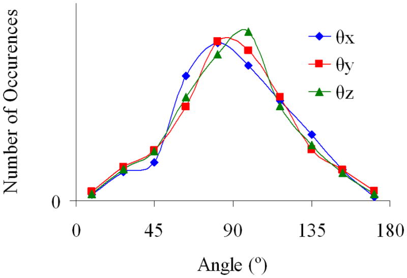
Histogram plot of direction cosine angles θx, θy, and θz for several random rotation matrices.

Ab initio electrostatic and polarization inter-molecular dimer energies are calculated with the RVS ^76,77 decomposition method using GAMESS⁷⁸. The ab initio electrostatic and polarization energies are compared to the corresponding energies calculated by molecular multipoles and polarizability tensors using expressions given by Stone⁶¹. A summary of these methods is given in Appendix C. In order for the multipole approximation to be valid, the inter-molecular density overlap of the molecules should be small. Since the exchange-repulsion energy is approximately proportional to the inter-molecular density overlap⁷⁹, only dimers in which the exchange-repulsion energy is less than 0.01 kcal/mol, are used.

III Results

1. Molecular Polarizability Tensor for Water

Molecular polarizability tensors up to the hexadecapole-hexadecapole level are calculated for water at the HF, B3LYP, and MP2 levels using the correlation consistent basis sets with additional augmented diffuse functions. Additional diffuse basis functions are important in calculating molecular polarizability tensors, since the electron charge density far away from the nuclei is more polarizable than the charge density near the nuclear centers. The z components of the dipole-dipole α_z;z, quadrupole-quadrupole C_zz;zz, octupole-octupole O_zzz;zzz, and hexadecapole-hexadecapole H_zzzz;zzzz polarizability tensor components calculated at the MP2 level are given in Tables III, IV, V, and VI respectively, as a function of increasing basis set size. For brevity, only the z components of the MP2 molecular polarizability tensors of rank l = l′ are listed. However, all components of the HF, B3LYP, and MP2 molecular polarizability tensors at different basis sets are given in the SI.

Table III.

α_z;z MP2 Water Dipole-Dipole Polarizability (bohr³)

X	aug-cc-pVXZ	d-aug-cc-pVXZ	t-aug-cc-pVXZ
D	9.044	9.692	9.679
T	9.484	9.719	9.727
Q	9.607	9.691	9.692
5	9.638	9.673	9.674
6	9.646	9.665	9.666

Table IV.

C_zz;zz MP2 Water Quadrupole-Quadrupole Polarizability (bohr⁵)

X	aug-cc-pVXZ	d-aug-cc-pVXZ	t-aug-cc-pVXZ
D	9.15	10.46	10.60
T	12.47	14.49	14.73
Q	13.54	14.68	14.69
5	14.05	14.64	14.63
6	14.32	14.61	14.61

Table V.

O_zzz;zzz MP2 Water Octupole-Octupole Polarizability (bohr⁷)

X	aug-cc-pVXZ	d-aug-cc-pVXZ	t-aug-cc-pVXZ
D	11.31	18.71	24.72
T	17.57	24.67	27.57
Q	21.56	30.04	31.02
5	24.28	30.50	30.79
6	25.94	30.54	30.65

Table VI.

H_zzzz;zzzz MP2 Water Hexadecapole-Hexadecapole Polarizability (bohr⁹)

X	aug-cc-pVXZ	d-aug-cc-pVXZ	t-aug-cc-pVXZ
D	4.20	10.69	*a
T	11.24	32.94	*
Q	19.09	43.53	57.58
5	26.48	53.60	61.22
6	32.73	54.57	60.42 (62.15)b

^aFor hexadecapole field perturbations, the SCF did not converge at the HF or B3LYP levels for the t-aug-cc-pVDZ and t-aug-cc-pVTZ basis sets.

^bThe value for H_zzzz;zzzz is given in parenthesis for the partially constructed q-aug-cc-pV6Z basis set (t6+).

The molecular polarizability tensor of lower multipole rank (e.g. dipole-dipole l = l′ = 1) converges faster with increasing basis set than polarizability tensors of higher multipole rank (e.g. hexadecapole-hexadecapole l = l′ = 4). For example from Table III, the smallest basis set aug-cc-pVDZ gives a reasonable estimate for the MP2 dipole-dipole polarizability of α_z;z = 9.044 bohr³ when compared to the value calculated by the largest t-aug-cc-pV6Z basis set of 9.666. The dipole-dipole polarizability converges relatively quickly when the basis set size is increased by including more polarization functions (α_z;z = 9.607 at MP2/aug-cc-pVQZ ) or including more diffuse shells (α_z;z = 9.692 at MP2/d-aug-cc-pVDZ).

In comparison, the quadrupole-quadrupole (l = l′ = 2) polarizability tensor converges more slowly with increasing basis set size than the dipole-dipole polarizability tensor. From Table IV, the smallest basis set aug-cc-pVDZ gives a less accurate estimate of C_zz;zz = 9.15 bohr⁵ forthe MP2 quadrupole-quadrupole polarizability when compared to the MP2/t-aug-cc-pV6Z result of 14.61. The d-aug-cc-pVTZ basis set gives a reasonable estimate of C_zz;zz = 14.49 bohr⁵.

The octupole-octupole (l = l′ = 3) polarizability O_zzz;zzz converges more slowly than the quadrupole-quadrupole polarizability. From Table V, the MP2/aug-cc-pVDZ result for O_zzz;zzz = 11.31 bohr⁷ can be compared to the MP2/t-aug-cc-pV6Z result of O_zzz;zzz = 30.65 bohr⁷. The d-aug-cc-pVQZ basis set gives a reasonable estimate of O_zzz;zzz = 30.04 bohr⁷.

The hexadecapole-hexadecapole (l = l′ = 4) H_zzzz;zzzz polarizability converges the slowest with increasing basis set size. From Table VI, the aug-cc-pVDZ basis set gives a poor estimate of H_zzzz;zzzz = 4.20 bohr⁹ when compared to the MP2/t-aug-cc-pV6Z result of H_zzzz;zzzz = 60.42 bohr⁹. It appears that the t-aug-cc-pV5Z basis set gives a reasonable estimate of H_zzzz;zzzz = 61.22 bohr⁹ when compared to the t-aug-cc-pV6Z result. In order to test the convergence of H_zzzz;zzzz at the t-aug-cc-pV6Z basis set, a fourth shell of diffuse functions is partially added the t-aug-cc-pV6Z basis set to give the ‘t6+’ basis set. At the MP2/t6+ level, H_zzzz;zzzz = 62.15 bohr⁹ indicating that H_zzzz;zzzz is reasonably converged at the t-aug-cc-pV5Z level. In addition, it should be noted that self-consistent field (SCF) convergence problems are found using the t-aug-cc-pVXZ (X = D,T) for hexadecapole field perturbations at both the HF and B3LYP levels.

Molecular polarizability tensors up to the quadrupole-quadrupole level are calculated at the HF, B3LYP, MP2, and CCSD levels with the d-aug-cc-pVQZ basis set and given in Table VII. The dipole-dipole polarizability xx, yy, and zz components of (8.976, 9.712, 9.310) bohr³ calculated at the CCSD/d-aug-cc-pVQZ level are in reasonably good agreement with previous CCSD calculations of (9.07, 9.77, 9.37) reported by Maroulis⁷¹ and of (9.05, 9.76, 9.37) reported by Avila⁷² using a basis set similar to that given by Maroulis⁷¹. In addition, Maroulis⁷¹ reports CCSD(T) dipole-dipole polarizabilites of (9.34, 9.93, 9.59). In this work, the dipole-dipole polarizability tensors calculated at the HF level are underestimated by 5–10% with respect to the more accurate CCSD calculations, while the dipole-dipole polarizability tensors calculated at the B3LYP level are overestimated by 5–10%. Interestingly, the MP2 results of (9.488, 9.942, 9.691) level slightly overestimates the molecular polarizabilities with respect to the CCSD level by 2–5% but agrees more with the CCSD(T) results reported by Maroulis⁷¹. Similar trends are found for the higher order dipole-quadrupole and quadrupole-quadrupole polarizability tensors. For completeness, dipole-quadrupole and quadrupole-quadrupole polarizability tensors reported in previous works^21,68–70 are also given in Table VII. The agreement between the HF dipole-quadrupole and quadrupole-quadrupole polarizabilities reported in this work and previous works^21,68,69 is mainly qualitative, since the d-aug-cc-pVQZ basis set used in this work contains s, p, d, f, g basis functions and is significantly larger than the basis sets used in the older works^21,68,69 which only contain s, p, d basis functions.

Table VII.

Water Molecular Polarizability Tensor^a (atomic units)

	HF	B3LYP	MP2	CCSD	Ref.
αxx	7.903	9.769	9.488	8.976	9.70e,	9.07f,	9.34g,	9.05h
αyy	9.186	10.204	9.942	9.712	10.06e,	9.77f,	9.93g,	9.76h
αzz	8.529	9.965	9.691	9.310	9.71e,	9.37f,	9.59g,	9.37h
Ax;xz	−0.42	−1.12	−1.08	−0.88	0.08b,	−0.03c,	−0.24d,	0.98e,
Ay;yz	−4.85	−5.47	−4.96	−5.01	−4.53b,	−4.93c,	−4.92d,	−2.08e
Az;xx	2.49	2.96	2.65	2.65	2.16b,	2.30c,	2.46d,	3.64e
Az;yy	−2.20	−2.06	−1.79	−2.00	−2.64b,	−2.50c,	−2.46d,	−3.25e
Az;zz	−0.29	−0.89	−0.86	−0.65	0.48b,	0.20c,	−0.01d,	−0.39e
Cxx;xx	13.47	18.23	16.27	15.18	8.57b,	10.13c,	11.83d,	13.73e
Cxx;yy	−7.12	−9.26	−8.31	−7.87	−5.05b,	−6.25c,	−6.88d,	−8.44e
Cxx;zz	−6.34	−8.96	−7.96	−7.30	−3.52b,	−3.88c,	−4.95d,	−5.29e
Cyy;yy	13.07	16.55	15.03	14.29	8.20b,	10.52c,	11.92d,	13.58e
Cyy;zz	−5.95	−7.29	−6.72	−6.42	−3.15b,	−4.27c,	−5.04d,	−5.14e
Czz;zz	12.30	16.26	14.68	13.72	6.67b,	8.15c,	9.99d,	10.43e
Cxy;xy	9.42	12.84	11.51	10.73	5.66b,	7.16c,	8.48d,	6.90e
Cxz;xz	9.45	12.97	11.59	10.75	5.33b,	6.09c,	4.64d,	5.99e
Cyz;yz	11.07	13.96	12.56	12.03	7.48b,	10.11c,	10.51d,	8.02e

^aThis Work. d-aug-cc-pVQZ = [7s6p5d4f3g/6s5p4d3f]

^bRef. 68 (1984), HF/[5s8p2d/2s1p]

^cRef. 21 (1987), HF/[6s5p3d/4s2p]

^dRef. 69 (1987), HF/(11s7p4d/5s2p1d)

^eRef. 70 (1994), CCSDT/[5s3p2d/3s2p]

^fRef. 71 (1998), CCSD/[9s6p6d3f/6s4p2d1f]

^gRef. 71 (1998), CCSD(T)/[9s6p6d3f/6s4p2d1f]

^hRef. 72 (2005), CCSD/[9s7p6d3f/6s5p2d1f]

As shown in Tables III – VI, the molecular polarizability tensors of lower multipole order l converge faster with increasing basis set than the polarizability tensors of higher multipole order. Using a heuristic argument, this trend can be explained in part by the angular momentum l used in basis functions. Ab initio basis sets are often constructed from spherically symmetric Gaussian type radial functions multiplied by a polynomial of degree l in x, y, z, which is associated with the angular momentum of the basis function. For example, in the aug-cc-pVTZ basis set, the oxygen atom has s, p, d, f basis functions corresponding to l = 0, 1, 2, 3 respectively. In the next higher level basis set of aug-cc-pVQZ, oxygen has s, p, d, f, g basis functions. The angular momentum l of the basis function is related to the multipole moments of the basis function. The ‘s’ basis functions are spherically symmetric, while the ‘p’ basis functions have non-zero dipole moments. Similarly, the ‘d’ and ‘f’ basis functions have non-zero quadrupole and octupole moments, respectively. Thus, accurate calculations of higher order multipole properties require basis sets composed of functions that have higher order multipole moments.

2. Test of the Molecular Multipole Approximation

In the previous section, the convergence of molecular polarizability tensors with respect to increasing basis set is investigated as a function of increasing multipole rank l. In this section, the convergence of long range intermolecular electrostatic and polarization energy calculated by molecular multipoles/polarizability tensors is investigated as a function of increasing multipole rank l at the HF/6-31++G** level. Ab initio electrostatic and polarization energies are calculated for randomly oriented small molecule dimers at the HF/6-31++G** level using the RVS method. The ab initio electrostatic and polarization energies are compared to energies calculated by molecular multipoles and polarizability tensors calculated at the HF/6-31++G** level. The dimers are separated into two sets: neutral-neutral dimers and neutral-charged dimers. The neutral molecules are NH₃, CH₃F, H₂C=O, and H₂O, while the charged ionic molecules are NH₄⁺, HCO₃⁻, and CO₃²⁻.

In Fig 2, scatter plots of inter-molecular electrostatic energies calculated by molecular multipoles up to rank l = 1, 2, 3 are compared with the reference HF/6-31++G** values for the neutral-neutral dimers. In Table VIII, the average magnitude of the electrostatic dimer energy <|E_{electrostatic}|> and the RMSD errors Δ_{electrostatic} in electrostatic dimer energy are given for l = 1, 2, 3, 4. For the neutral-neutral dimers, the value <|E_{electrostatic}|> = 0.267 kcal/mol can be compared to the RMSD errors Δ_{electrostatic} = 0.120, 0.028, 0.0070, and 0.0038 (kcal/mol) for molecular multipoles up to rank l = 1, 2, 3, 4, respectively. The corresponding percent errors (RMSD/<|E_ele|>) are 45%, 10%, 2.6%, and 1.4% for molecular multipoles up to rank l = 1, 2, 3, 4, respectively. For the neutral-charge dimers, the corresponding percent errors in electrostatic dimer energy are 19%, 4.1%, 0.85%, and 0.28% for molecular multipoles up to rank l = 1, 2, 3, 4, respectively. In both sets of dimers, a systematic increase in precision is obtained by increasing the multipole rank of the molecular multipole moments from l = 1 to l = 4.

Figure 2.

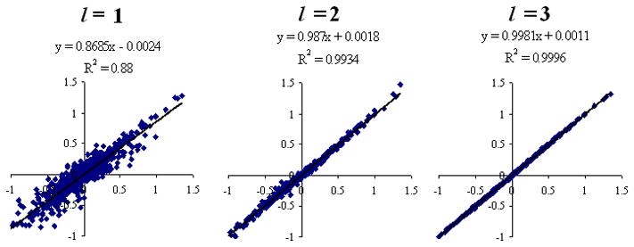
Long range electrostatic energies (kcal/mol) calculated by molecular multipoles up to rank l = 1, 2, 3 for randomly oriented neutral-neutral dimers at the HF/6-31++G** level.

Table VIII.

RMSD errors (Δ) and average magnitudes (<|E|>) in electrostatic energy and polarization energy (kcal/mol) calculated molecular multipoles and molecular polarizability tensors up to rank l = 1, 2, 3, 4 for randomly oriented neutral-neutral and neutral-charge dimers at the HF/6-31++G** level

Neutral-Neutral Dimers			Neutral-Charge Dimers
l	Δelectrostatic	Δpolarization	Δelectrostatic	Δpolarization
1	0.12032	0.001674	0.45475	0.03217
2	0.02836	0.000630	0.10014	0.00985
3	0.00702	0.000237	0.02072	0.00274
4	0.00385	0.000129	0.00681	0.00229
<|E|>	0.267	0.00425	2.431	0.136

Similarly, scatter plots of polarization energy calculated by molecular polarizability tensors up to rank l = 1, 2, 3 are compared to their reference HF/6-31++G** values in Figs 3 and 4 for the neutral-neutral and neutral-charged dimers, respectively. Molecular multipoles up to hexadecapole (l = 4) are used as the source for electrostatic field in the calculation of polarization energies. In Table VIII, the average magnitudes <|E_polarization|>and the RMSD errors in polarization energy Δ_polarization are given for both the neutral-neutral and the neutral-charged dimers. For the neutral-neutral dimers, the percent errors in polarization energy are 39%, 15%, 5.5%, and 3.0% for molecular polarizability tensors up to rank l = 1, 2, 3, 4, respectively. For the neutral-charged dimers, the percent errors in polarization energy are 24%, 7.2%, 2.0%, and 1.7% for molecular polarizability tensors up to rank l = 1, 2, 3, 4, respectively. As expected, a significant increase in precision is obtained by increasing the multipole rank of the molecular polarizability tensors from l = 1 to l = 4.

Figure 3.

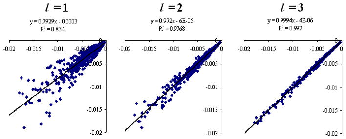
Long range polarization energies (kcal/mol) calculated by molecular polarizability tensors up to rank l = 1, 2, 3 and molecular multipoles up to hexadecapoles (l = 4) for randomly oriented neutral-neutral dimers at the HF/6-31++G** level.

Figure 4.

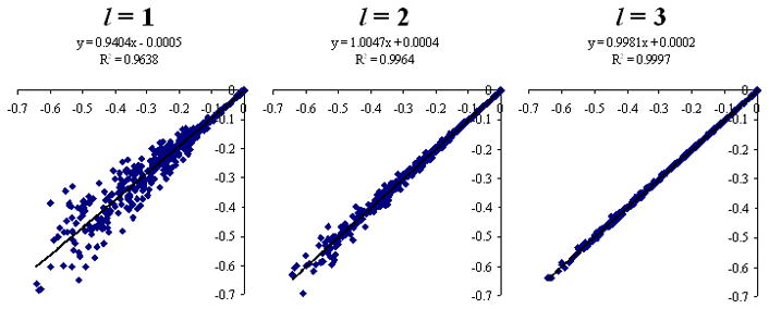
Long range polarization energies (kcal/mol) calculated by molecular polarizability tensors up to rank l = 1, 2, 3 and molecular multipoles up to hexadecapoles (l = 4) for randomly oriented neutral-charge dimers at the HF/6-31++G** level.

IV Conclusion

In this work, a finite field procedure for calculating molecular polarizability tensors of arbitrary multipole rank is proposed. Mathematical expressions for converting ‘pure’ Cartesian, traceless Cartesian, and spherical tensor multipoles and polarizability tensors are derived for arbitrary multipole rank. We have implemented the finite field method for calculating molecular polarizability tensors up to hexadecapole-hexadecapole using output files obtained from the Gaussian⁸⁵ suite of quantum chemistry programs. In addition, molecular polarizability tensors calculated by MOLPRO in the ‘pure’ Cartesian tensor form are converted to spherical tensor and traceless Cartesian forms.

As an example, molecular polarizability tensors are calculated for water at the HF, B3LYP, and MP2 levels up to hexadecapole-hexadecapole with the correlation consistent basis sets. It is shown that as the multipole rank l is increased, the polarizability converges more slowly with basis set size. In addition, dipole-dipole, dipole-quadrupole, and quadrupole-quadrupole polarizability tensors are calculated for water at the CCSD/d-aug-cc-pVQZ level and compared to previous works.

The molecular multipole approximation is tested on randomly oriented small molecule dimers separated by a large distance. Inter-molecular electrostatic and polarization energies calculated by molecular multipoles and polarizability tensors are compared to their ab initio reference values. A systematic increase in accuracy and precision is demonstrated in going from the molecular dipole approximation (l = 1) to the molecular hexadecapole approximation (l = 4). Although the molecular multipoles and polarizability tensors calculated at the HF level do not include electron correlation and the 6-31++G** basis set may not be converged with respect to the complete basis set limit, the calculations demonstrate the significance of including higher order molecular multipoles in reproducing ab initio electrostatic and polarization energies.

The formal results presented in this paper should prove useful to those engaged in the study of inter-molecular interactions by either high level calculation or approximation schemes. In particular, the method for obtaining molecular polarizability tensors of arbitrary multipole rank for arbitrary molecular systems and the formulae developed for inter-converting multipoles and polarizabilities between various tensor standards should prove invaluable.

Appendix

A. Mathematical Background

A spherical harmonic function Y_lm (θ,φ) is defined on a unit sphere (θ,φ) in terms of Associated Legendre functions^62,86 P_lm (cos θ) by

$$Y_{lm}(\theta ,\phi )\equiv {(-1)}^m\sqrt{\frac{2l+1}{4\pi }}\sqrt{\frac{(l-m)!}{(l+m)!}}{P}_{lm}(cos\theta )e^{im\phi }$$ (A.1)

Hobson⁶² has derived an especially useful polynomial expression for P_lm (cos θ) as

$$P_{lm}(cos\theta )=\frac{(l+m)!}{2^m}\sum _{k=0}^{\left[\frac{l-m}{2}\right]}{\left(\frac{-1}{4}\right)}^k\frac{{cos}^{l-m-2k}\theta {sin}^{m+2k}\theta }{(l-m-2k)!(m+k)!k!}$$ (A.2)

for 0 ≤ m ≤ l. A regular solid harmonic function C_lm is defined over all space r by

$$C_{lm}(\mathbf{r})\equiv r^l\sqrt{\frac{4\pi }{2l+1}}{Y}_{lm}(\theta ,\phi ).$$ (A.3)

A polynomial expression for C_lm (x, y, z) for 0 ≤ m ≤ l can be derived by inserting eqns. A.1 and A.2 in A.3

$$C_{lm}(\mathbf{r})={(-1)}^m\frac{A_{lm}}{2^m}\sum _{k=0}^{\left[\frac{l-m}{2}\right]}{\left(\frac{-1}{4}\right)}^k\frac{z^{l-m-2k}{(x+iy)}^{m+k}{(x-iy)}^k}{(l-m-2k)!(m+k)!k!}$$ (A.4)

where

$$A_{lm}\equiv \sqrt{(l+m)!(l-m)!}.$$ (A.5)

An important symmetry for solid harmonic functions is given by

$$C_{lm}^{\ast }(\mathbf{r})={(-1)}^m{C}_{l-m}(\mathbf{r})$$ (A.6)

By taking into account eqn. A.6, the expression for C_lm (x, y, z) in eqn. A.4 becomes valid for −l ≤ m ≤ l by

$$C_{lm}(\mathbf{r})={(-1)}^{m_{+}}\frac{A_{lm}}{2^{\mid m\mid }}\sum _{k=0}^{\left[\frac{l-\mid m\mid }{2}\right]}{\left(\frac{-1}{4}\right)}^k\frac{z^{l-\mid m\mid -2k}{(x+iy)}^{m_{+}+k}{(x-iy)}^{m_{-}+k}}{(l-\mid m\mid -2k)!(m_{+}+k)!(m_{-}+k)!}$$ (A.7)

where m_± ≡ (|m| ± m)/2. After expanding (x + iy)^m₊+k and (x–iy)^m₋+k, eqn. A.7 becomes

$$C_{lm}(\mathbf{r})=\sum _{k=0}^{\left[\frac{l-\mid m\mid }{2}\right]}\sum _{p=0}^{k+m_{+}}\sum _{q=0}^{k+m_{-}}{a}_{k,p,q}^{lm}{x}^{p+q}{y}^{\mid m\mid +2k-p-q}{z}^{l-\mid m\mid -2k}$$ (A.8)

where

$$a_{k,p,q}^{lm}\equiv \frac{{(-1)}^{\mid m\mid +q}{A}_{lm}}{2^{\mid m\mid +2k}(l-\mid m\mid -2k)!p!(k+m_{+}-p)!q!(k+m_{-}-q)!}{i}^{\mid m\mid +2k-p-q}$$ (A.9)

The solid harmonic gradient operator C_lm (λ) is defined by replacing r with its partial derivatives

$$C_{lm}(\nabla )\equiv \sum _{k=0}^{\left[\frac{l-\mid m\mid }{2}\right]}\sum _{p=0}^{k+m_{+}}\sum _{q=0}^{k+m_{-}}{a}_{k,p,q}^{lm}{\left(\frac{\partial }{\partial x}\right)}^{p+q}{\left(\frac{\partial }{\partial y}\right)}^{\mid m\mid +2k-p-q}{\left(\frac{\partial }{\partial z}\right)}^{l-\mid m\mid -2k}$$ (A.10)

Transformation formulae between C_lm (r) and ${\widehat{\zeta }}_{l_x{l}_y{l}_z}^{(l)}(\mathbf{r})$ (eqn. 24) are derived in the Supplementary Information and given by

$${\widehat{\zeta }}_{l_x{l}_y{l}_z}^{(l)}(\mathbf{r})=\sum _{n=0}^{l_x+l_y}{b}_n^{l_x,l_y,l}{C}_{l,2n-l_x-l_y}(\mathbf{r})$$ (A.11)

$$C_{lm}(\mathbf{r})=\sum _{k=0}^{\mid m\mid }{c}_k^{lm}{\widehat{\zeta }}_{\mid m\mid -k,k,l-\mid m\mid }^{(l)}(\mathbf{r})$$ (A.12)

where $b_n^{l_x,l_y,l}$ and $c_k^{lm}$ are constants given by

$$b_n^{l_x,l_y,l}\equiv \frac{i^{l_y}{A}_{l,2n-l_x-l_y}}{2^{l_x+l_y}l!}\sum _{q=max(0,n-l_x)}^{min(l_y,n)}\left(\begin{array}{c}{l}_x\\ n-q\end{array}\right)\left(\begin{array}{c}{l}_y\\ q\end{array}\right){(-1)}^{n+q}$$ (A.13)

$$c_k^{lm}\equiv \{\begin{array}{cc}\frac{l!{(-1)}^{m_{+}}}{A_{lm}}\left(\begin{array}{c}\mid m\mid \\ k\end{array}\right)i^k& m\ge 0\\ \frac{l!{(-1)}^k}{A_{lm}}\left(\begin{array}{c}\mid m\mid \\ k\end{array}\right)i^k& m<0\end{array}$$ (A.14)

Suppose r̂ = (sin θ cos φ, sin θ sin φ, cos θ) is a point on a unit sphere and R̄ is a Cartesian rotation matrix which transforms r̂, i.e. r̂′ = R̄·r̂ is another point on a unit sphere. Spherical harmonics are functions of r̂ and transform under rotations as

$$Y_{lm}(\overline{\mathbf{R}}·\widehat{\mathbf{r}})=\sum _{m^{\prime }=-l}^l{D}_{m^{\prime }m}^l[{\overline{\mathbf{R}}}^{-1}]Y_{{lm}^{\prime }}(\widehat{\mathbf{r}})$$ (A.15)

where D^l_m′m is a Wigner⁸⁸ function. Solid harmonic functions C_lm(r) are defined over all space r= rr̂. The rotational properties for C_lm(r) follow from eqns. A.3 and A.15 as

$$C_{lm}(\overline{\mathbf{R}}·\mathbf{r})=\sum _{m^{\prime }=-l}^l{D}_{m^{\prime }m}^l[{\overline{\mathbf{R}}}^{-1}]C_{{lm}^{\prime }{lm}^{\prime }{lm}^{\prime }}(\mathbf{r})$$ (A.16)

In addition, solid harmonic functions transform under translation through the following addition theorem⁸⁹

$$C_{lm}({\mathbf{r}}_1+{\mathbf{r}}_2)=\sum _{l^{\prime }=0}^l\sum _{m^{\prime }=-l^{\prime }}^{l^{\prime }}{B}_{l^{\prime }{m}^{\prime }}^{lm}{C}_{l^{\prime }{m}^{\prime }}({\mathbf{r}}_1)C_{l-l^{\prime },m-m^{\prime }}({\mathbf{r}}_2)$$ (A.17)

where $B_{l^{\prime }{m}^{\prime }}^{lm}$ is a constant defined by

$$B_{l^{\prime }{m}^{\prime }}^{lm}\equiv \frac{A_{lm}}{A_{l^{\prime }{m}^{\prime }}{A}_{l-l^{\prime },m-m^{\prime }}}$$ (A.18)

and A_lm is a constant defined in eqn. A.5.

B. Rotation/Translation Formulae for Multipoles and Polarizabilities

Rotation and translation formulae for multipoles and polarizabilities follow from eqns. A.16 and A.17, respectively. The following expressions are useful, for example, if multipoles or polarizabilities are rotated between different orientations or translated between different molecular centers.

Suppose a molecule with charge density ρ(r) is rotated to another orientation defined by a 3x3 Cartesian rotation matrix R̄. The rotated molecule has charge density ρ(R̄⁻¹·r) and multipoles with respect to the origin (R = 0) given by

$$\begin{array}{l}{Q}_{lm}^{\mathit{rot}}=\int d^3\mathbf{r}\rho ({\overline{\mathbf{R}}}^{-1}·\mathbf{r})C_{lm}(\mathbf{r})\\ =\int d^3{\mathbf{r}}^{\prime }\rho ({\mathbf{r}}^{\prime })C_{lm}(\overline{\mathbf{R}}·{\mathbf{r}}^{\prime })\end{array}$$ (B.1)

where the variable r have been transformed to r′= R̄⁻¹·r (note the Jacobian is 1 since det(R̄)=1). Inserting eqn. A.16 into eqn. B.1 gives

$$Q_{lm}^{\mathit{rot}}=\sum _{m^{\prime }=-l}^l{D}_{m^{\prime }m}^{(l)}[{\overline{\mathbf{R}}}^{-1}]Q_{{lm}^{\prime }}$$ (B.2)

where Q_lm are the multipoles of the unrotated molecule. Starting with eqn. 11, polarizabilities with respect to the origin (R = 0) transform under rotations as

$$\begin{array}{l}{\alpha }_{l_1{m}_1;l_2{m}_2}^{\mathit{rot}}=-\iint d^3{\mathbf{r}}_1{d}^3{\mathbf{r}}_2\eta ({\overline{\mathbf{R}}}^{-1}·{\mathbf{r}}_1,{\overline{\mathbf{R}}}^{-1}·{\mathbf{r}}_2)C_{l_1{m}_1}({\mathbf{r}}_1)C_{l_2{m}_2}({\mathbf{r}}_2)\\ =\sum _{{m_1}^{\prime }=-l_1}^{l_1}\sum _{{m_2}^{\prime }=-l_2}^{l_2}{D}_{{m_1}^{\prime }{m}_1}^{(l_1)}[{\overline{\mathbf{R}}}^{-1}]D_{{m_2}^{\prime }{m}_2}^{(l_2)}[{\overline{\mathbf{R}}}^{-1}]{\alpha }_{l_1{m_1}^{\prime };l_2{m_2}^{\prime }}\end{array}$$ (B.3)

where α_l1m1;l2m2 are the polarizabilities of the unrotated molecule.

A multipole with respect to the center R₁ is defined by eqn. 10 as

$$Q_{lm}^1=\int d^3\mathbf{r}\rho (\mathbf{r})C_{lm}(\mathbf{r}-{\mathbf{R}}_1)$$ (B.4)

Q¹_lm can be expressed in terms of multipoles with respect to a different center R₂ by applying the addition theorem (eqn. A.17) to C_lm(r – R₁)

$$C_{lm}(\mathbf{r}-{\mathbf{R}}_1)=\sum _{l^{\prime }=0}^l\sum _{m^{\prime }=-l^{\prime }}^{l^{\prime }}{B}_{l^{\prime }{m}^{\prime }}^{lm}{C}_{l^{\prime }{m}^{\prime }}(\mathbf{r}-{\mathbf{R}}_2)C_{l-l^{\prime },m-m^{\prime }}({\mathbf{R}}_{21})$$ (B.5)

where R₂₁ ≡ R₂ – R₁. Inserting eqn. B.5 into eqn. B.4 results in a translation formulae form multipoles.

$$Q_{lm}^1=\sum _{l^{\prime }=0}^l\sum _{m^{\prime }=-l^{\prime }}^{l^{\prime }}{B}_{l^{\prime }{m}^{\prime }}^{lm}{C}_{l-l^{\prime },m-m^{\prime }}({\mathbf{R}}_{21})Q_{l^{\prime }{m}^{\prime }}^2$$ (B.6)

Similarly, polarizabilities with respect to R₂ can be translated to R₁ by

$${\alpha }_{l_1{m}_1;l_2{m}_2}^1=\sum _{{l_1}^{\prime }=0}^{l_1}\sum _{{m_1}^{\prime }=-{l_1}^{\prime }}^{{l_1}^{\prime }}\sum _{{l_2}^{\prime }=0}^{l_2}\sum _{{m_2}^{\prime }=-{l_2}^{\prime }}^{{l_2}^{\prime }}{B}_{{l_1}^{\prime }{m_1}^{\prime }}^{l_1{m}_1}{B}_{{l_2}^{\prime }{m_2}^{\prime }}^{l_2{m}_2}{C}_{l_1-{l_1}^{\prime },m_1-{m_1}^{\prime }}({\mathbf{R}}_{21})C_{l_2-{l_2}^{\prime },m_2-{m_2}^{\prime }}({\mathbf{R}}_{21}){\alpha }_{{l_1}^{\prime }{m_1}^{\prime };{l_2}^{\prime }{m_2}^{\prime }}^2$$ (B.7)

C. Multipole Electrostatic/Polarization Dimer Energies

In this section, results given by Stone⁶¹ are briefly summarized. The electrostatic energy between two molecules A and B is given by

$$U_{\mathit{ele}}=\sum _{lm}{Q}_{lm}^A{\varphi }_{lm}^{0\ast }({\mathbf{R}}_A)$$ (C.1)

where $Q_{lm}^A$ is the set of multipoles of molecule A in the global frame (see eqn. C.6 below). The permanent field on molecule A (denoted by 0 superscript) due to the multipoles on molecule B is given by

$${\varphi }_{lm}^{0\ast }({\mathbf{R}}_A)=\sum _{l^{\prime }{m}^{\prime }}{T}_{lm;l^{\prime }{m}^{\prime }}({\mathbf{R}}_A-{\mathbf{R}}_B)Q_{l^{\prime }{m}^{\prime }}^B$$ (C.2)

The interaction matrix T_lm;l′m′ is given by

$$T_{lm;l^{\prime }{m}^{\prime }}(\mathbf{r})\equiv {(-1)}^{l^{\prime }}\sqrt{\frac{4\pi }{2L+1}}\sqrt{\left(\begin{array}{c}L+M\\ l+m\end{array}\right)\left(\begin{array}{c}L-M\\ l-m\end{array}\right)}\frac{Y_{LM}^{\ast }(\widehat{\mathbf{r}})}{r^{L+1}}$$ (C.3)

where Y_LM is a spherical harmonic, L ≡ l + l′, and M ≡ m + m′. A similar expression is given for the permanent field on molecule B.

The polarization energy between molecules A and B is given by

$$U_{\mathit{pol}}=\frac{1}{2}\sum _{lm}{\mathrm{\Delta }}_{lm}^A{\varphi }_{lm}^{0\ast }({\mathbf{R}}_A)+{\mathrm{\Delta }}_{lm}^B{\varphi }_{lm}^{0\ast }({\mathbf{R}}_B)$$ (C.4)

where ${\mathrm{\Delta }}_{lm}^A$ and ${\mathrm{\Delta }}_{lm}^B$ are the induced molecular multipoles for molecules A and B. In the calculation of ab initio second order polarization energies, the permanent vacuum charge density of one molecule polarizes the other molecule (and vice-versa). In other words, the induced charge densities do not polarize one another until self-consistency at second order. When comparing to the ab inito results, the induced multipoles were polarized by permanent molecular multipoles. For example, the induced multipole on molecule A is given by

$${\mathrm{\Delta }}_{lm}^A=-\sum _{l^{\prime }{m}^{\prime }}{\alpha }_{lm;l^{\prime }{m}^{\prime }}^A{\varphi }_{l^{\prime }{m}^{\prime }}^{0\ast }({\mathbf{R}}_A)$$ (C.5)

where ${\alpha }_{lm;l^{\prime }{m}^{\prime }}^A$ is the ab initio molecular polarizability tensor of molecule in the ‘global frame’ (see eqn. C.7 below) and ${\varphi }_{l^{\prime }{m}^{\prime }}^{0\ast }({\mathbf{R}}_A)$ is the electrostatic field gradients on molecule A due to the permanent molecular multipoles on molecule B given by eqn. C.2. A similar expression exists for molecule B.

The ab initio molecular multipoles and polarizability tensors are calculated in a ‘local’ reference frame with respect to the origin R = 0, which also coincides with the molecular center of mass. The ‘local’ and ‘global’ reference frame concept^28,61,90 has been used in models based on atomic multipoles. In the randomly oriented dimer geometries, the molecular multipoles and polarizability tensors are rotated to the ‘global’ reference frame of the molecule in the dimer geometry. The ‘local’ frame multipoles $Q_{{lm}^{\prime }}^L$ transform to ‘global’ frame multipoles $Q_{lm}^G$ through Wigner rotation matrices⁸⁸ $D_{m^{\prime }m}^{(l)}$ by

$$Q_{lm}^G=\sum _{m^{\prime }}{D}_{m^{\prime }m}^{(l)}[{\overline{\mathbf{R}}}^{-1}]Q_{{lm}^{\prime }}^L$$ (C.6)

where R̄ is a 3x3 Cartesian rotation matrix⁹⁰ describing the ‘local’ to ‘global’ frame transformation. Similarly, the ‘local’ frame molecular polarizability tensors transform to ‘global’ frame molecular polarizability tensors by

$${\alpha }_{l_1{m}_1;l_2{m}_2}^G=\sum _{{m_1}^{\prime }=-l_1}^{l_1}\sum _{{m_2}^{\prime }=-l_2}^{l_2}{D}_{{m_1}^{\prime }{m}_1}^{(l_1)}[{\overline{\mathbf{R}}}^{-1}]D_{{m_2}^{\prime }{m}_2}^{(l_2)}[{\overline{\mathbf{R}}}^{-1}]{\alpha }_{l_1{m_1}^{\prime };l_2{m_2}^{\prime }}^L$$ (C.7)

References

- 1.Buckingham AD, Pople JA. Proc Phys Soc (London) 1955;A68:905. [Google Scholar]
- 2.Buckingham AD. J Chem Phys. 1959;30:1580–1585. [Google Scholar]
- 3.Buckingham AD. Quart Rev. 1959;13:183–214. [Google Scholar]
- 4.McLean AD, Yoshimine M. J Chem Phys. 1967;47(6):1927–1935. [Google Scholar]
- 5.Buckingham AD, Utting BD. Annu Rev Phys Chem. 1970;21:287–316. [Google Scholar]
- 6.Böttcher CJF. Theory of electric polarization. 2. Elsevier Scientific Pub. Co; New York, NY: pp. 1973–87. [Google Scholar]
- 7.Gray CG, Lo BWN. Chem Phys. 1976;14:73–87. [Google Scholar]
- 8.Applequist J. Chem Phys. 1984;85:279–290. [Google Scholar]
- 9.Stone AJ. Chem Phys Lett. 1988;155(1):102–110. [Google Scholar]
- 10.Dykstra CE. J Comput Chem. 1988;9(5):476–487. [Google Scholar]
- 11.Maroulis G, Pouchan C. Chem Phys Lett. 2008;464:16–20. [Google Scholar]
- 12.Hohm U, Maroulis G. J Chem Phys. 2006;124(12):124312–6. doi: 10.1063/1.2181141. [DOI] [PubMed] [Google Scholar]
- 13.Hohm U, Maroulis G. J Chem Phys. 2004;121(21):10411–10418. doi: 10.1063/1.1809607. [DOI] [PubMed] [Google Scholar]
- 14.Cohen HD, Roothaan CCJ. J Chem Phys. 1965;43(10):S34–S39. [Google Scholar]
- 15.Maroulis G, Bishop DM. Chem Phys Lett. 1985;114(2):182–186. [Google Scholar]
- 16.Bishop DM, Pipin J, Lam B. Chem Phys Lett. 1986;127(4):377–380. [Google Scholar]
- 17.Bishop DM, Pipin J. Theor Chim Acta. 1987;71:247–253. [Google Scholar]
- 18.Maroulis G, Thakkar AJ. J Chem Phys. 1988;88(12):7623–7632. [Google Scholar]
- 19.Dykstra CE. J Chem Phys. 1985;82(9):4120–4125. [Google Scholar]
- 20.Liu S, Dykstra CE. Chem Phys Lett. 1985;119(5):407–411. [Google Scholar]
- 21.Liu S, Dykstra CE. J Phys Chem. 1987;91:1749–1754. [Google Scholar]
- 22.Dykstra CE, Jasien PC. Chem Phys Lett. 1984;109(4):388–393. [Google Scholar]
- 23.Millot C, Stone AJ. Mol Phys. 1992;77(3):439–462. [Google Scholar]
- 24.Millot C, Soetens JC, Costa MTCM, Hodges MP, Stone AJ. J Phys Chem A. 1998;102:754–770. [Google Scholar]
- 25.Batista ER, Xantheas SS, Jonsson H. J Chem Phys. 1998;109(11):4546–4551. [Google Scholar]
- 26.Stern H, Rittner F, Berne B, Friesner R. J Chem Phys. 2001;115:2237–2251. [Google Scholar]
- 27.Burnham CJ, Xantheas SS. J Chem Phys. 2002;16:1500–1510. [Google Scholar]
- 28.Ren P, Ponder JW. J Phys Chem B. 2003;107:5933–5947. [Google Scholar]
- 29.Torheyden M, Jansen G. Mol Phys. 2006;104:2101–2138. [Google Scholar]
- 30.Bukowski R, Szalewicz K, Groenenboom GC, van der Avoird A. Science. 2007;315:1249–1252. doi: 10.1126/science.1136371. [DOI] [PubMed] [Google Scholar]
- 31.Defusco A, Schofield DP, Jordan KD. Mol Phys. 2007;105:2681–2696. [Google Scholar]
- 32.Mankoo PK, Keyes T. J Chem Phys. 2008;129:034504–9. doi: 10.1063/1.2948966. [DOI] [PubMed] [Google Scholar]
- 33.Burnham CJ, Anick DJ, Mankoo PK, Reiter GF. J Chem Phys. 2008;128:154519–20. doi: 10.1063/1.2895750. [DOI] [PubMed] [Google Scholar]
- 34.Kumar R, Wang F, Jenness GR, Jordan KD. J Chem Phys. 2010;132:014309–12. doi: 10.1063/1.3276460. [DOI] [PubMed] [Google Scholar]
- 35.Appleqquist J, Carl JR, Fung KK. J Am Chem Soc. 1972;94(9):2952–2960. [Google Scholar]
- 36.Thole BT. Chem Phys. 1981;59:341–350. [Google Scholar]
- 37.Elking DM, Darden T, Woods RJ. J Comput Chem. 2007;28:1261–1274. doi: 10.1002/jcc.20574. [DOI] [PMC free article] [PubMed] [Google Scholar]
- 38.Lamoureux G, MacKerell AD, Roux B. J Chem Phys. 2003;119:5185–5197. [Google Scholar]
- 39.Rick SW, Stuart SJ, Berne BJ. J Chem Phys. 1994;101:6141–6156. [Google Scholar]
- 40.Stern HA, Kaminski GA, Banks JL, Zhou R, Berne BJ, Friesner RA. J Phys Chem. 1999;103:4730–4737. [Google Scholar]
- 41.Patel S, Brooks CL., III J Comput Chem. 2004;25:1–16. doi: 10.1002/jcc.10355. [DOI] [PubMed] [Google Scholar]
- 42.Patel S, MacKerell AD, Brooks CL., III J Comput Chem. 2004;25:1504–1514. doi: 10.1002/jcc.20077. [DOI] [PubMed] [Google Scholar]
- 43.Truchon JF, Nicholls A, Iftimie RI, Roux B, Bayly CI. J Chem Theory Comput. 2008;4(9):1480–1493. doi: 10.1021/ct800123c. [DOI] [PMC free article] [PubMed] [Google Scholar]
- 44.Truchon JF, Nicholls A, Iftimie RI, Roux B, Bayly CI. J Chem Theory Comput. 2009;5(7):1785–1802. doi: 10.1021/ct900029d. [DOI] [PMC free article] [PubMed] [Google Scholar]
- 45.Stone AJ. Mol Phys. 1985;56(5):1065–1082. [Google Scholar]
- 46.Le Sueur CR, Stone AJ. Mol Phys. 1993;78(5):1267–1291. [Google Scholar]
- 47.Le Sueur CR, Stone AJ. Mol Phys. 1994;83(2):293–307. [Google Scholar]
- 48.Misquitta AJ, Stone AJ. J Chem Phys. 2006;124:024111–14. doi: 10.1063/1.2150828. [DOI] [PubMed] [Google Scholar]
- 49.Parr RG, Yang W. Density Functional Theory of Atoms and Molecules. Oxford University Press; New York, NY: 1994. [Google Scholar]
- 50.McWeeny R. Methods of Molecular Quantum Mechanics. Academic Press; San Diego, USA: 1998. [Google Scholar]
- 51.Stone AJ. Chem Phys Lett. 1981;83(2):233–239. [Google Scholar]
- 52.Stone AJ. J Chem Theory Comput. 2005;1(6):1128–1132. doi: 10.1021/ct050190+. [DOI] [PubMed] [Google Scholar]
- 53.Celebi N, Angyan J, Dehez F, Millot C, Chipot C. J Chem Phys. 2000;112(6):2709–2717. [Google Scholar]
- 54.Williams GJ, Stone AJ. J Chem Phys. 2000;119(9):4620–4628. [Google Scholar]
- 55.Misquitta AJ, Stone AJ, Price SL. J Chem Theory Comput. 2008;4:19–32. doi: 10.1021/ct700105f. [DOI] [PubMed] [Google Scholar]
- 56.Holt A, Karlstrom G. J Comput Chem. 2008;29:2033–2038. doi: 10.1002/jcc.20976. [DOI] [PubMed] [Google Scholar]
- 57.Holt A, Bostrom J, Karlstrom G, Lindh R. J Comput Chem. 2010;31:1583–1591. doi: 10.1002/jcc.21502. [DOI] [PubMed] [Google Scholar]
- 58.Amos RD, Alberts IL, Andrews JS, Colwell SM, Handy NC, Jayatilaka D, Knowles PJ, Kobayashi R, Laidig KE, Laming G, Lee AM, Maslen PE, Murray CW, Rice JE, Simandiras ED, Stone AJ, Su MD, Tozer DJ. CADPAC: The Cambridge Analytic Derivatives Package Issue 6. Cambridge: 1995. [Google Scholar]
- 59.Werner H-J, Knowles PJ, Manby FR, Schutz M, Celani P, Knizia G, Korona T, Lindh R, Mitrushenkov A, Rauhut G, Adler TB, Amos RD, Bernhardsson A, Berning A, Cooper DL, Deegan MJO, Dobbyn AJ, Eckert F, Goll E, Hampel C, Hesselmann A, Hetzer G, Hrenar T, Jansen G, Koppl C, Liu Y, Lloyd AW, Mata RA, May AJ, McNicholas SJ, Meyer W, Mura ME, Nicklas A, Palmieri P, Pfluger K, Pitzer R, Reiher M, Shiozaki T, Stoll H, Stone AJ, Tarroni R, Thorsteinsson T, Wang M, Wolf A. MOLPRO [Google Scholar]
- 60.Angeli C, Bak KL, Bakken V, Christiansen O, Cimiraglia R, Coriani S, Dahle P, Dalskov EK, Enevoldsen T, Fernandez B, Hattig C, Hald K, Halkier A, Heiberg H, Helgaker T, Hettema H, Jensen HJ, Jonsson D, Jorgensen P, Kirpekar S, Klopper W, Kobayashi R, Koch H, Ligabue A, Lutnas OB, Mikkelsen KV, Norman P, Olsen J, Packer MJ, Pedersen TB, Rinkevicius Z, Rudberg E, Ruden TA, Ruud K, Salek P, Sanchez de Meras A, Saue T, Sauer SPA, Schimmelpfennig B, Sylvester-Hvid KO, Taylor PR, Vahtras O, Wilson DJ, Agren H. DALTON Release 2 [Google Scholar]
- 61.Stone AJ. The Theory of Intermolecular Forces. Oxford University Press; Oxford, UK: 2000. [Google Scholar]
- 62.Hobson EW. The Theory of Spherical and Ellipsoidal Harmonics. Chelsea; New York, NY: 1955. [Google Scholar]
- 63.Cipriani J, Silvi B. Mol Phys. 1982;45(2):259–272. [Google Scholar]
- 64.Özdođan T. J Math Chem. 2006;42(2):201–214. [Google Scholar]
- 65.Woon DE, Dunning TH. J Chem Phys. 1993;98(2):1358–1371. [Google Scholar]
- 66.Woon DE, Dunning TH. J Chem Phys. 1994;100(4):2975–2988. [Google Scholar]
- 67.Feller D. J Comput Chem. 1996;17(13):1571–1586. https://bse.pnl.gov/bse/portal.
- 68.Dacre PD. J Chem Phys. 1984;80(11):5677–5683. [Google Scholar]
- 69.Bishop DM, Pipin J. Theor Chim Acta. 1987;71:247–253. [Google Scholar]
- 70.Pluta T, Noga J, Bartlett RJ. Int J Quant Chem. 1994;28:379–393. [Google Scholar]
- 71.Maroulis G. Chem Phys Lett. 1998;289:403–411. [Google Scholar]
- 72.Avila G. J Chem Phys. 2005;122:144310–10. doi: 10.1063/1.1867437. [DOI] [PubMed] [Google Scholar]
- 73.Murphy WF. J Chem Phys. 1977;67(12):5877–5882. [Google Scholar]
- 74.Bishop DM. Rev Mod Phys. 1990;62(2):343–374. [Google Scholar]
- 75.London F. Z Phys. 1930;63:245. [Google Scholar]
- 76.Stevens WJ, Fink WH. Chem Phys Lett. 1987;139(1):15–22. [Google Scholar]
- 77.Chen W, Gordon MS. J Phys Chem. 1996;100:14316–14328. [Google Scholar]
- 78.Schmidt MW, Baldridge KK, Boatz JA, Elbert ST, Gordon MS, Jensen JJ, Koseki S, Matsunaga N, Nguyen KA, Su S, Windus TL, Dupuis M, Montgomery JA GAMESS Version 21 Nov. 1994. J Comput Chem. 1993;4:1347. [Google Scholar]
- 79.Wheatley RJ, Price SL. Mol Phys. 1990;69:507–533. [Google Scholar]
- 80.Szabo A, Ostlund NS. Modern Quantum Chemistry: Introduction to Advanced Electronic Structure. Dover Publications; Mineola, NY: 1996. [Google Scholar]
- 81.Diercksen GHF, Sadlej AJ. J Chem Phys. 1981;75(3):1253–1266. [Google Scholar]
- 82.Diercksen GHF, Roos BO, Sadlej A. J Chem Phys. 1981;59:29–39. [Google Scholar]
- 83.Handy NC, Schaefer HF., III J Chem Phys. 1984;81(11):5031–5033. [Google Scholar]
- 84.Wiberg KB, Hadad CM, LePage TJ, Breneman CM, Frisch MJ. J Phys Chem. 1992;96:671–679. [Google Scholar]
- 85.Frisch MJ, Trucks GW, Schlegel HB, Scuseria GE, Robb MA, Cheeseman JR, Montgomery JA, Jr, Vreven T, Kudin KN, Burant JC, Millam JM, Iyengar SS, Tomasi J, Barone V, Mennucci B, Cossi M, Scalmani G, Rega N, Petersson GA, Nakatsuji H, Hada M, Ehara M, Toyota K, Fukuda R, Hasegawa J, Ishida M, Nakajima T, Honda Y, Kitao O, Nakai H, Klene M, Li X, Knox JE, Hratchian HP, Cross JB, Bakken V, Adamo C, Jaramillo J, Gomperts R, Stratmann RE, Yazyev O, Austin AJ, Cammi R, Pomelli C, Ochterski JW, Ayala PY, Morokuma K, Voth GA, Salvador P, Dannenberg JJ, Zakrzewski VG, Dapprich S, Daniels AD, Strain MC, Farkas O, Malick DK, Rabuck AD, Raghavachari K, Foresman JB, Ortiz JV, Cui Q, Baboul AG, Clifford S, Cioslowski J, Stefanov BB, Liu G, Liashenko A, Piskorz P, Komaromi I, Martin RL, Fox DJ, Keith T, Al-Laham MA, Peng CY, Nanayakkara A, Challacombe M, Gill PMW, Johnson B, Chen W, Wong MW, Gonzalez C, Pople JA. Gaussian 03, Revision C.02. Gaussian, Inc; Wallingford CT: 2003. [Google Scholar]
- 86.Arfken GB. Mathematical Methods for Physicists. 5. Academic Press; San Diego, CA: 2000. [Google Scholar]
- 87.Rowe EGP. J Math Phys. 1978;19:1962–1968. [Google Scholar]
- 88.Varshalovich DA, Moskalev AN, Khersonskii VK. Quantum Theory of Angular Momentum. World Scientific; Singapore: 1988. [Google Scholar]
- 89.Chakrabarti S, Dewangan DP. J Phys B: At Mol Opt Phys. 1995;28:L769–L774. [Google Scholar]
- 90.Elking DM, Perera L, Duke R, Pedersen LG. J Comput Chem. 2010;31(15):2702–2713. doi: 10.1002/jcc.21563. [DOI] [PMC free article] [PubMed] [Google Scholar]
- 91.Benedict WS, Gailar N, Plyler EK. J Chem Phys. 1956;24(6):1139–1165. [Google Scholar]
Associated Data
This section collects any data citations, data availability statements, or supplementary materials included in this article.