Modified Watershed Technique and Post-Processing for Segmentation of Skin Lesions in Dermoscopy Images

Abstract

In previous research, a watershed-based algorithm was shown to be useful for automatic lesion segmentation in dermoscopy images, and was tested on a set of 100 benign and malignant melanoma images with the average of three sets of dermatologist-drawn borders used as the ground truth, resulting in an overall error of 15.98%. In this study, to reduce the border detection errors, a neural network classifier was utilized to improve the first-pass watershed segmentation; a novel “Edge Object Value (EOV) Threshold” method was used to remove large light blobs near the lesion boundary; and a noise removal procedure was applied to reduce the peninsula-shaped false-positive areas. As a result, an overall error of 11.09% was achieved.

1. Introduction

Lesion segmentation is a critical step in the automated analysis of digital dermoscopy images [1]. In previous research, Chen and Wang et al. implemented a watershed-based approach for automatic skin lesion segmentation in dermoscopy images, incorporating pre- and post-processing steps to reduce errors [2, 3]. The method of Chen, although yielding a low average border error of 5.3%, required 44 features for classifier determination of the border. Additionally, the error for Chen’s watershed implementation was compared to the boundaries determined by only a single dermatologist. The method of Wang et al. required no classifier and compared the automatic watershed borders to the average of three dermatologists’ borders, but the average border error was 15.98%. In this research, we use the same set of 100 contact-dermoscopy images used in previous studies and improve Wang’s and Chen’s methods by implementing three post-processing steps: 1) minimizing false peninsulas using an adaptive mathematical morphology technique, 2) removing large bright areas at the lesion boundary using a novel adaptive edge object value threshold, and 3) using a supervised neural network with feature selection added to reduce the errors by improving the lesion ratio estimate. Details of the basic watershed implementation are given in Wang et al. [3]. The remainder of this paper is organized into the following sections: 1) description of the watershed algorithm, 2) object merging using a lesion ratio estimate, 3) border smoothing, and 4) conclusion.

2. Watershed algorithm for lesion segmentation

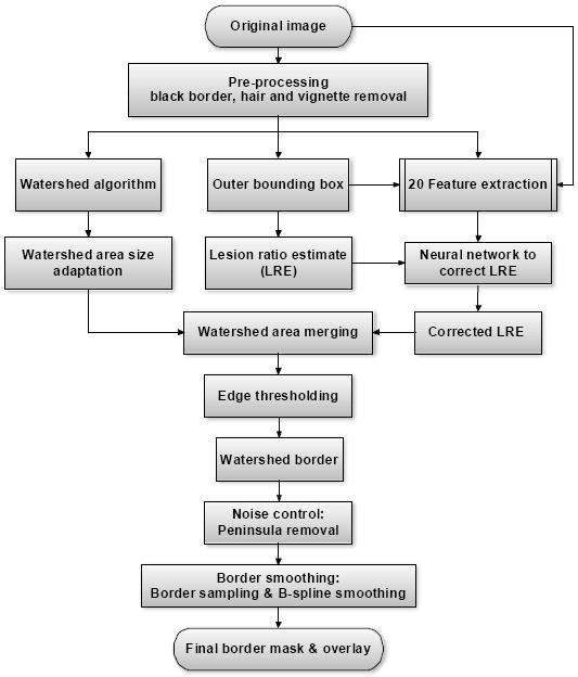
Figure 1 presents the flowchart of the watershed algorithm explored in this study. Each individual component will be discussed in following sections.

Fig. 1.

Lesion border segmentation using watershed algorithm flowchart.

2.1 Preprocessing: hair removal, vignette removal and black border removal

Hair, vignetting and black borders are three main types of noise in dermoscopy images that can affect the watershed merging procedure. A morphological closing operator is implemented to remove the hairs. Pixels darker than average in areas of high deviation in luminance are detected. Areas with a high concentration of these pixels are considered to be hair [3]. The vignetting effect (darkened image corners due to position-dependent loss of brightness in the output of an optical system) is minimized by a three-step brightness adjustment procedure. First, a set of concentric circular regions is defined. Then, starting at the image center, the brightness of the next circular region is adjusted so that the average intensity is the same as the center. This procedure continues for every region [3]. Black borders were cropped by determining the innermost point of the black rim at each corner of the image and then cropping [3].

2.2 Watershed algorithm

The watershed algorithm is an image segmentation algorithm based on the theory of mathematical morphology [4]. The watershed algorithm uses an intensity-based topographical representation in which the brighter pixels represent higher altitudes or the ‘hills’ and the darker pixels correspond to the ‘valleys,’ which allows for the determination of the path that a falling raindrop would follow. Watershed lines are the divide lines of ‘domains of attraction’ of water drops (or the boundaries of catchment basins). The flooding modification of the watershed algorithm is analogous to immersion of the relief in a lake flooded from holes at minima. This variant is more efficient than the original falling raindrop approach for many applications [3].

3. Lesion ratio estimate (LRE) and objects merging

3.1. LRE based on outer bounding box algorithm

The LRE is based on the outer bounding box ratio, which is the ratio of the area of the outer bounding box to the whole image area. Three formulas are used to determine the outer bounding box:

The vertical projection of the image is a function of the horizontal index j:

$$p_j={\sum }_{i=1}^n{I}_{\mathit{ij}}$$ (1)

Let p_f be the best-fit quadratic function created from the projection curve p_j:

$$p_f=a_2{x}^2+a_{1}x+a_0$$ (2)

To obtain the final subtraction equation, the means of the curves p¯_f and p¯_J are used to normalize the curve, yielding the final equation of the bounding curve B_j:

$$B_j=[p_j-(p_f-\overline{p_f})]\frac{p_j}{\overline{p_J}}$$ (3)

The maxima of B_j on each side of the global minimum provide the horizontal limits of the bounding box. A similar procedure provides the vertical limits of the bounding box [3]. Instead of processing the entire image as in Chen’s implementation [2], only the center of the image is processed, from 25% to 75% of the image height and width, saving up to 75% of the running time. Based on the outer bounding box, we established the relationship between the outer bounding box ratio and the new lesion ratio as NewLRE = B · 0.8633 − 0.1919, where B, the outer bounding box ratio, is the ratio of the bounding box area to the image area in the same manner as in [3], that is by finding the best-fit line based on the data from the 100-image data set. The entire data set was used because it was felt that with such a small data set, the entire set was needed to produce the best-fit line.

3.2 LRE correction based on neural network

The Random Forest data mining algorithm [5] was used in previous research to optimize the segmentation, using 44 features from the original images as inputs [2]: image area (in pixels); first-iteration lesion area (in pixels); gray levels of the high and low peaks of the object histogram (the histogram of the average gray levels of the watershed objects where watershed objects are the green, blue and luminance (R, G, B, L) (where luminance is defined as L = 0.299R + 0.587G + 0.114B; image pixel means; entire image pixel standard deviations; first watershed rim averages, i.e. the average intensity over the area between the borders determined by lesion ratio estimates γ and γ + 0.01 (using watershed segmentation in all four planes); mean LRE γ̂_L (the number of image pixels that have higher luminance than the mean luminance of the image in all four planes); pixel histogram x- and y-axis peak values, where pixel histogram refers to the histogram of the entire image in each of the four planes; pixel histogram variances and standard deviations (that is, the variances and standard deviations of the histogram functions in each of the four planes, not the pixel variances and standard deviations) and the average grayscale of the inner and outer bounding boxes. In this study, a supervised back-propagation neural network approach is explored for enhancing the segmentation accuracy. A feature selection procedure was carried out to eliminate the less significant/redundant features. Step-wise logistic regression (implemented in SAS [6], a statistical analysis software package) was used to select the best features by finding those with the lowest Chi-square value. SAS picked a total of 17 features: mean R and B values at the watershed rim (two features); average R, G, B values for the image (three features); peak G, B values of the object histogram (two features); pixel histogram standard deviation in B and L planes (two features); pixel histogram variance in L plane (one feature); inner bounding box in B plane (one feature); entire image pixel standard deviations in R, G, B and L planes (four features); the average intensity over the area between the borders determined by lesion ratio estimates γ and γ + 0.01 (using watershed segmentation in B plane) (one feature); and mean LRE in B plane (one feature). A dermatologist then added some features he considered essential and removed some similar features from the 17-feature set, resulting in a 20-feature set that performed better than the 17-feature set. The twenty features used are: mean R and B values at the watershed rim (two features); average R, G, B values for the image (three features); peak R, G, B values of the object histogram (three features); blue plane LRE (one feature); pixel histogram standard deviation in B and L planes (two features); pixel histogram variance in L plane (one feature); and the inner and outer bounding box R, G, B and L averages (eight features). Using these features as inputs, a feed-forward neural network using the back propagation training method is used to classify the lesion ratio estimate into one of three classes: proper estimate, over estimate (by 5% or more), and under estimate (by 5% or more). The network has twenty neurons with linear transfer functions and one bias neuron in the input layer, five neurons with (unipolar) sigmoid transfer functions in the hidden layer and one neuron in the output layer with a hyperbolic tangent transfer function at the neuron output. The learning gain is 0.2; momentum gain is 0.1. The training procedure stops when the root mean square error of the output is under 0.1 or when it reaches 100 epochs. The final lesion ratio estimate is given by:

$$\gamma ={\widehat{\gamma }}_B+0.025\cdot pp=\{\begin{array}{cc}0\hfill & \hfill \mathrm{proper\; estimate}\\ -1\hfill & \hfill \mathrm{over\; estimate}\\ 1\hfill & \hfill \mathrm{under\; estimate}\end{array}$$

where γ = final LRE and γ̂_B = bounding box (first) LRE. For the first LRE, the average error value is 15.98%. The average lesion ratio is about 0.25 (ratio of lesion area to the image area), so 2.5% of image area is around 10% of the lesion area. The value of 0.025 indicates adding or subtracting 2.5% of the image area. The neural network thresholded outputs of -1, 0, and 1 are classes that stand for over estimate, proper estimate and under estimate. A feed-forward back-propagation neural network was applied for data classification. The entire set of 100 images was randomly divided into ten disjoint subsets retaining the same ratio of malignant to benign images in each subset. Nine subsets (ninety images) were used as the training set and one subset (ten images) was used as the test set. The subsets were then rotated so that each subset was used as the test set exactly once. The result reported here is the average of these ten runs. The supervised neural network correctly classified 70% of the images into the three classes.

4. Object merging and border smoothing

4.1 Edge object value threshold and merging

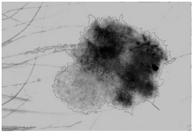
Large bright edge blobs at the boundary can introduce errors in the merging procedure. If the magnitude of the gradient near the lesion edge is not large, i.e. if the pixel gray levels change gradually, after the watershed approach large bright watershed objects can exist with the smaller part of the object inside the lesion and the larger part outside the lesion. In most cases, a false positive error results. One method to solve this problem is to use a threshold on an adaptive “edge object value (EOV)” defined as: EOV = R× A/B, where R = mean watershed object blue value, A = watershed object area size in pixels, and B = average lesion blue value. During the merging procedure, a watershed object at the edge of the current lesion boundary with an EOV above the threshold is not merged into the lesion area. Empirically, the EOV threshold was optimized at a value of 50,000 to eliminate large bright areas. This resulted in falsely eliminated areas in some lesions. Figure 2 shows the merged watershed objects and the lesion contour overlaid after applying the edge object value threshold procedure.

Fig. 2.

Edge object value threshold and primary watershed border overlay.

4.2 Border smoothing

4.2.1 Peninsula noise removal

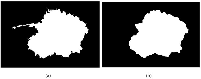
Peninsula noise (Figure 3(a)) is reduced by erosion followed by dilation with a circular structuring element proportional to the lesion size (Figure 3(b)), where the structuring element radius is given by $R=k\sqrt{A}$, where k is a tunable parameter (a value of 0.05 worked well) and A = lesion area. This operation of erosion followed by dilation with the same structuring element is also called opening.

Fig. 3.

Peninsula removal: (a) primary watershed border; (b) peninsula removed border.

4.2.2 B-Spline border smoothing and final border overlay

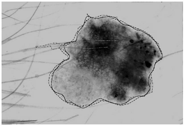
Second-order B-Spline closed-curve fitting [7] is applied to the peninsula-smoothed border of the lesion mask. Compared to intervals of 8 and 16, which work better for jagged borders, a distance of 32 was selected for the B-Spline smoothing interval. Average control points for the B-Spline are calculated at a distance of 32 pixels (in either the x- or y-direction, whichever occurs first) along the border (based on experimentation using 8-, 16- and 32-pixel distances) for the B-Spline smoothing interval [3]. In Figure 4, the solid line is the final watershed border after the border-smoothing method is applied, the dashed line is the average of three sets of manually-drawn borders, and the dash-dot line shows the watershed border without the peninsula removal process and neural network classification. Using an XOR operation to calculate the area error, this image gives a total error of 7.180% with 6.310% false negative and 0.8700% false positive.

Fig. 4.

Final border overlay: dermatologist border (dashed), watershed border without post-processing [3] (dash-dot), and final watershed border (solid)

5. Results

Three dermatologists manually determined lesion borders on all 100 images. The average of the three dermatologists’ borders was obtained using a distance transform summing method, as follows. First, a Euclidean distance transform was obtained of the interior of each dermatologist’s lesion (pixels on the border of the lesion were assigned a value of one and points farther in were assigned higher numbers). Those values count as votes for that pixel being a lesion pixel. Second, the same procedure was applied for the outside of the lesion counting those values as votes against. Then, the votes were tallied (the distance transforms were summed with the skin values as negatives). Ties were chosen to be lesion. As shown in Table 1, when compared with the average dermatologist border, our watershed method had a mean percentage border error of 11.09% (benign error of 11.00%, melanoma error of 11.53%, and an overall error of 11.09%) based on the 100-image set. The median and maximum errors for each group are: 9.16% and 34.55% for benign, 10.35% and 20.54% for melanoma, and 9.56% and 34.55% for overall.

Table 1.

Watershed border error statistics

Dermatologist	Diagnosis	Mean	Median	Maximum
Stoecker	Benign	0.1408	0.1222	0.3637
	Melanoma	0.1253	0.1108	0.2344
	Total	0.1363	0.1177	0.3637
Malters	Benign	0.1131	0.1002	0.3861
	Melanoma	0.1369	0.1131	0.4445
	Total	0.1200	0.1071	0.4445
Grichnik	Benign	0.1239	0.1086	0.4358
	Melanoma	0.1306	0.1244	0.2364
	Total	0.1259	0.1139	0.4358
Average	Benign	0.1100	0.0916	0.3455
	Melanoma	0.1153	0.1035	0.2054
	Total	0.1109	0.0956	0.3455

In Table 2, the watershed error is lower than the error obtained by the Gradient Vector Flow (GVF) snake method (benign 13.77%, melanoma 19.76%, and overall 15.59% using the numbers from one dermatologist’s borders) [8]. The watershed error is similar to that obtained with the J measure based SEGmentation (JSEG) method [9] on the same set of images (benign 10.83%, melanoma 13.75%, and overall 11.58%). The borders from the GVF snake method [8] and the Independent Histogram Pursuit (IHP) method [10] were compared with the border of only one dermatologist in the results given above. The IHP and Statistical Region Merging (SRM) [11] methods worked better than the watershed approach; however, the IHP method [10] was compared with only one dermatologist’s border and the SRM method [11] used a 90-image subset of the 100 images. The error metric used was the one developed by Hance et al. [12] and used in [3]. A number of studies have used the same image database for dermoscopy image segmentation [7-10, 13-15]. Some of the cited studies are not compared to the watershed method here because they used a different error metric.

Table 2.

Watershed border error comparison (–: data unavailable)

Dermatologist	Diagnosis	GVF	IHP	SRM	JSEG	Watershed
		100 images	100 images	90 images	100 images	100 images
Stoecker	Benign	0.1377	0.0321	0.1138	0.1083	0.1408
	Melanoma	0.1976	0.0253	0.1029	0.1375	0.1253
	Total	0.1559	0.0273	0.1111	0.1158	0.1363
Malters	Benign	–	–	0.1017	0.1082	0.1131
	Melanoma	–	–	0.1050	0.1298	0.1369
	Total	–	–	0.1027	0.1137	0.1200
Grichnik	Benign	–	–	0.1056	0.1226	0.1239
	Melanoma	–	–	0.1041	0.1341	0.1306
	Total	–	–	0.1052	0.1255	0.1259
Average	Benign	–	–	–	–	0.1100
	Melanoma	–	–	–	–	0.1153
	Total	–	–	–	–	0.1109

6. Conclusion

The watershed algorithm can segment skin lesions with high accuracy. The lesion ratio estimate and bounding box methods from [2] provide important additional information added to the watershed algorithm to control the lesion size, allowing correction of errors made at the first iteration. Using these tools, a supervised neural network was then implemented to further diminish the segmentation error. Novel post-processing steps presented here included adaptive morphological peninsula clipping and adaptive bright area merging thresholds.

References

- 1.Celebi ME, Iyatomi H, Schaefer G, Stoecker WV. Lesion border detection in dermoscopy images. Comput Med Imaging Graphics. 2009;33:148–153. doi: 10.1016/j.compmedimag.2008.11.002. [DOI] [PMC free article] [PubMed] [Google Scholar]
- 2.Chen X. Ph D Dissertation. Dept. of Electrical and Computer Engineering, University of Missouri-Rolla; 2007. Skin lesion segmentation by an adaptive watershed flooding approach. [Google Scholar]
- 3.Wang H, Moss RH, Chen X, Stanley RJ, Stoecker WV, Celebi ME, et al. Segmentation of skin lesions in dermoscopy images using a watershed technique. Skin Res Technol. 2010;16:378–384. doi: 10.1111/j.1600-0846.2010.00445.x. [DOI] [PMC free article] [PubMed] [Google Scholar]
- 4.Meyer F, Beucher S. Morphological Segmentation. J Vis Commun Image R. 1990;1:21–46. [Google Scholar]
- 5.Breiman L. Random Forests. Mach Learn. 2001;45:5–32. [Google Scholar]
- 6.SAS Institute, Inc.; Cary, NC, USA: [Google Scholar]
- 7.de Boor C. A Practical Guide to Splines. New York, NY: Springer-Verlag; 2001. [Google Scholar]
- 8.Erkol B, Moss RH, Stanley RJ, et al. Automatic lesion boundary detection in dermoscopy images using gradient vector flow snakes. Skin Res Technol. 2005;11:17–26. doi: 10.1111/j.1600-0846.2005.00092.x. [DOI] [PMC free article] [PubMed] [Google Scholar]
- 9.Celebi ME, Aslandogan YA, Stoecker WV, et al. Unsupervised border detection in dermoscopy images. Skin Res Techol. 2007;13:454–462. doi: 10.1111/j.1600-0846.2007.00251.x. [DOI] [PMC free article] [PubMed] [Google Scholar]
- 10.Delgado D, Butakoff C, Ersboll BK, Stoecker WV. Independent Histogram Pursuit for Segmentation of Skin Lesions. IEEE Transactions on Biomedical Engineering. 2008;55:157–161. doi: 10.1109/TBME.2007.910651. [DOI] [PMC free article] [PubMed] [Google Scholar]
- 11.Celebi ME, Kingravi H, Iyatomi H, Aslandogan A, Stoecker WV, Moss RH. Border Detection in Dermoscopy Images Using Statistical Region Merging. Skin Res Technol. 2008;14:347–353. doi: 10.1111/j.1600-0846.2008.00301.x. [DOI] [PMC free article] [PubMed] [Google Scholar]
- 12.Hance GA, Umbaugh SE, Moss RH, Stoecker WV. Unsupervised color image segmentation with application to skin tumor borders. IEEE Eng Med Biol. 1996;15:104–111. [Google Scholar]
- 13.Zhou H, Schaefer G, Sadka A, Celebi ME. Anisotropic Mean Shift Based Fuzzy C-Means Segmentation of Dermoscopy Images. IEEE Journal of Selected Topics in Signal Processing. 2009;3:26–34. [Google Scholar]
- 14.Celebi ME, Schaefer G, Iyatomi H, Stoecker WV, Malters JM, Grichnik JM. An Improved Objective Evaluation Measure for Border Detection in Dermoscopy Images. Skin Res Technol. 2009;15:444–450. doi: 10.1111/j.1600-0846.2009.00387.x. [DOI] [PMC free article] [PubMed] [Google Scholar]
- 15.Zhou H, Schaefer G, Celebi ME, Lin F, Liu T. Gradient vector flow with mean shift for image segmentation. Comput Med Imag Graph. 2010 doi: 10.1016/j.compmedimag.2010.08.002. in press, this issue, pages at proof time. [DOI] [PubMed] [Google Scholar]