Interactive, Computer-Assisted Tracking of Speckle Trajectories in Fluorescence Microscopy: Application to Actin Polymerization and Membrane Fusion

Abstract

Analysis of particle trajectories in images obtained by fluorescence microscopy reveals biophysical properties such as diffusion coefficient or rates of association and dissociation. Particle tracking and lifetime measurement is often limited by noise, large mobilities, image inhomogeneities, and path crossings. We present Speckle TrackerJ, a tool that addresses some of these challenges using computer-assisted techniques for finding positions and tracking particles in different situations. A dynamic user interface assists in the creation, editing, and refining of particle tracks. The following are results from application of this program: 1), Tracking single molecule diffusion in simulated images. The shape of the diffusing marker on the image changes from speckle to cloud, depending on the relationship of the diffusion coefficient to the camera exposure time. We use these images to illustrate the range of diffusion coefficients that can be measured. 2), We used the program to measure the diffusion coefficient of capping proteins in the lamellipodium. We found values ∼0.5 μm²/s, suggesting capping protein association with protein complexes or the membrane. 3), We demonstrate efficient measuring of appearance and disappearance of EGFP-actin speckles within the lamellipodium of motile cells that indicate actin monomer incorporation into the actin filament network. 4), We marked appearance and disappearance events of fluorescently labeled vesicles to supported lipid bilayers and tracked single lipids from the fused vesicle on the bilayer. This is the first time, to our knowledge, that vesicle fusion has been detected with single molecule sensitivity and the program allowed us to perform a quantitative analysis. 5), By discriminating between undocking and fusion events, dwell times for vesicle fusion after vesicle docking to membranes can be measured.

Introduction

Advances in microscopic imaging continues to create unique demands for particle tracking in biological systems (1–4). Examples of tasks that involve tracking of bright spots include virus trafficking in live cells (5), motion of transmembrane proteins on the cell membrane (6), cell microrheology (3,4), dynamics and fusion of secretory and synaptic vesicles (7–10), and tracking of cytoskeletal proteins (11–14).

The field of algorithm development for particle tracking has a rich history. There are three approaches to apply these algorithms to biological systems. First, close collaboration among biologists, computer scientists, and physical scientists to develop specialized software (2). Second, many labs resort to commercial software. The latter, however, have the disadvantage that they are expensive, often require additional modules, and need to be modified by the vendor. Finally, a third possibility is to use open-source software tools that may be directly applied, or depending on the flexibility of the program, modified for a specific system.

One of the first freely available particle tracking tools was developed in IDL (15,16) to track the positions of colloidal particles. This algorithm involved image restoration followed by detection of particle positions and linking of positions into trajectories. This code has been converted to the MATLAB (The MathWorks, Natick, MA) and C++ languages and extended in three dimensions (17,18). It has also been adapted in the MATLAB program PolyParticleTracker (19). GMimPro is a detection and tracking software available as a compiled Windows program (20,21). Freely available MATLAB code for particle tracking further includes u-track (22), MTT (23), and plusTipTracker (24) (optimized for tracking microtubule plus-ends). The programs “u-track” and “MTT”, developed for tracking dense particle systems, use various criteria for deciding the likelihood of particle merging, starting, stopping, and gaps in detection failure.

Because the MATLAB platform is not always available, many researchers have contributed tracking algorithms as plug-ins for the open-source image analysis program ImageJ (National Institutes of Health, Bethesda, MD). Some open-source plug-ins are MTrack2, Manual Tracking, and Particle Tracker (25). The latter is based on the MATLAB code and methods developed in Sbalzarini and Koumoutsakos (26). Free ImageJ plug-ins, available as .jar files (compiled code), include MTrackJ (27) and SpotTracker (28).

All tracking algorithms start failing at low signal/noise ratio (S/N) and at high particle mobility during camera exposure. These challenging situations are common in single molecule studies in live cells (11,29). Another challenge occurs when one is interested in a small subset of particles within a heterogeneous population, such as single vesicles that fuse with the plasma membrane or with supported bilayers (7–10,30). The challenge is to track only that subset. In all those cases, the primary question is whether valid single particle tracks can be obtained at all.

To address the above challenges we developed an open-source particle-tracking tool, Speckle TrackerJ, as an ImageJ plug-in (31), with the following two-tier strategy:

• 1.Tracks are obtained with rough positioning accuracy, using user assistance and supervision when needed.
• 2.The positioning accuracy and precision of the existing tracks are improved.

This iterative approach is much more efficient than trying to achieve the best tracking performance in a single step in the challenging cases described above. The user can control which of the candidate particles to track over time with the aid of tracking models. We designed models that use the expected behavior of particles to improve detection and tracking. A modular construction allows modification and design of new tracking models. Our method is particularly useful when measuring particle lifetimes—i.e., trajectory length—in the presence of noise and blinking where user input is required to distinguish broken trajectories from real appearance and disappearance events.

We demonstrate that Speckle TrackerJ compares well with related software in control synthetic image sequences that cover a range of noise levels and particle mobilities. We then proceed to demonstrate the successful application of our method to four different challenging experimental situations: 1), dynamics of single capping proteins at the leading edge of motile cells; 2), single-molecule actin speckle lifetimes in lamellipodia; 3), release and diffusion of single fluorescent lipids from vesicles upon fusion with supported, planar bilayers; and 4), docking-to-fusion lifetimes of vesicles fusing with planar-supported bilayers mediated by soluble n-ethylmaleimide-sensitive factor attachment protein receptor (SNARE) proteins. In none of these situations could other existing software be used satisfactorily.

Materials and Methods

Particle representation

Trajectories of particles through time are recorded as speckle tracks. Each point of a track is represented by a speckle mark. Tracks can be created and modified by a user or through computer-assisted techniques. Computer-assisted tracking is divided into three steps: Step 1), detection of speckle mark candidates; Step 2), tracking through time to create a speckle track using a model; and Step 3), refinement of speckle mark positions. These steps can be repeated manually or using batch tracking. At any point during this process, the speckle tracks can be modified (see User Interface section in the Supporting Material).

Detecting particles

We implemented two detection methods:

• 1.Locate-Speckles. Uses a threshold value to create a binary image. A two-pass connected components algorithm is then applied to find speckle mark candidates.
• 2.Template-Locate. Performs the same operation as the Locate-Speckles method except that it uses existing speckle marks to create a normalized cross-correlation (NCC) filtered copy of the image. The NCC template is created by averaging a square region of adjustable size centered at existing speckle marks.

Tracking

Tracking has been separated into two components: the tracker algorithm (see Fig. S2 in the Supporting Material) and the tracker models. The tracker algorithm applies the selected model successively from frame to frame and records which speckle tracks are being modified; models modify speckle tracks by adding new marks (some only refine their position).

Tracker algorithm

Before the tracker starts, it initializes the selected model with existing speckle tracks (which tracks are used depends on the model). After initialization, the tracker creates a tracking list, a list of speckle tracks to be updated. The tracking loop begins by passing a speckle track and the current timeframe to the model, which then determines how to continue to the track. If the model determines that a track ends, the track is removed from the list. After the model finishes, the tracker checks the tracking list for speckle tracks that overlap. Overlap occurs if two tracks have a speckle mark on the same frame and the distance between those marks is less than a user-adjustable minimum distance parameter. If the tracking list is not empty, the tracker will move to the next frame and start the tracking loop again.

Tracker models

We implemented tracking models that use fixed and adaptable parameters (see Supporting Material and (31)). Adaptable-parameter models “learn” as tracking proceeds.

Diffusing-Spots is an adaptable-parameter model that adds a new mark to the speckle track in the frame immediately after the last frame that has already been marked. It searches for a new mark within a square region centered at the previous mark. The model is initialized by calculating the average intensity, 〈I〉, the variance in intensity, σ_δI², and the variance in frame to frame displacement, σ_d², calculated using all speckle marks from either the selected speckle track, if Auto-Track was used to start the tracker, or all existing tracks, if Auto-Track All was used. The intensity measurements are made by integrating the pixel intensity over a circle centered at the position of each speckle mark. The radius is a user-adjustable parameter. To predict the position of the next speckle mark, the model finds all pixels that are local maxima within the square search region. For each candidate location, the intensity, I, change in intensity from the previous frame, δI, and the displacement from the previous frame, d, is measured and used to generate weights,

$$\begin{array}{l}{w}_i=e^{\left(I-\langle I\rangle \right)/\left(\langle I\rangle -I_m\right)},\\ w_{\delta I}=e^{-\delta I^2/\left(2{\sigma }_{\delta I}^2\right)},\\ w_d=e^{-d^2/\left(2{\sigma }_d^2\right)},\end{array}$$ (1)

where I_m is the mean value of the intensity in all frames of the movie being analyzed. If I is >〈I〉, w_i is set to 1. The weights are summed with user-adjustable factors, f_i, f_δI, and f_d, to get a combined weight:

$$w=w_i{f}_i+w_{\delta I}{f}_{\delta I}+w_d{f}_d,f_i+f_{\delta I}+f_d=1.$$ (2)

The best candidate is accepted if w > w_min. If no candidate satisfies this condition, the track stops.

Diffusing-NCC is similar to Diffusing-Spots but it takes into account NCC values. Initialization consists of measuring the average intensity I over a circle and NCC value at every speckle mark position using a square template made from all speckle marks. To find a new candidate location, the model checks the square search region for the location with the maximum NCC value. Then the intensity and NCC value are measured at that location and used in a weighting function

$$w=e^{-\left[{\left(I-\langle I\rangle \right)}^2/\left(2{\sigma }_I^2\right)\right]}{e}^{-\alpha \left[{\left(NCC-\langle NCC\rangle \right)}^2/\left(2{\sigma }_{NCC}^2\right)\right]},$$ (3)

where averages and standard deviations are over all existing speckle marks and α is an adjustable parameter. If w is smaller than a threshold w_min, the track ends.

The Constant-Velocity-NCC model is the same as Diffusing NCC but the search for the best candidate occurs over a square whose center is displaced from the position of the previous speckle mark. This method is useful in cases where particles move with constant velocity.

Refine position

Speckle tracks can be refined to improve the position of existing speckle marks (see Supporting Material). The Adjustment model modifies existing speckle tracks by moving them to the center of intensity. The Gaussian-Fit model refines the position of speckles with subpixel accuracy by fitting a two-dimensional Gaussian to the intensity near a speckle mark.

Experiments

Details of experimental protocols can be found in Supporting Material. In summary, live cell imaging of XTC cells was carried out as described in Miyoshi et al. (29). Fluorescent speckle microscopy was carried out by observing cells expressing a low amount of EGFP-tagged proteins. Imaging acquisition was carried out at 21–23°C using PlanApo 100× (NA 1.40) or 150× (NA 1.45) oil objectives (Olympus, Melville, NY).

Single-vesicle docking and fusion experiments were performed as described in detail in Karatekin et al. (32). Synaptic/exocytic vesicle-associated v-SNARE proteins VAMP2/synaptobrevin and the target membrane associated t-SNAREs syntaxin and SNAP25 were reconstituted into small unilamellar vesicles (SUVs) and planar, supported bilayers (SBLs), respectively. The SUVs carry a small fraction of fluorescently labeled lipids. We used total internal reflection fluorescence microscopy (TIRFM) at 31 frames/s full-frame (512 × 512 pixels) or at 57 frames/s from a 400 × 256 pixel region of interest using a back-thinned electron-multiplying charge-coupled device camera (iXon DU897E; Andor Technology, Belfast, Northern Ireland).

Results

Speckle TrackerJ was designed with the ability to correctly follow multiple moving particles over their lifetimes in the presence of inhomogeneous backgrounds, noise, particle crossings, and multiple sources of intensity fluctuations. We have, however, implemented standard methods for subpixel particle localization, such as two-dimensional Gaussian fitting. In Fig. 1 we demonstrate how the localization accuracy ε of our program depends on S/N and pixel size (26,33) (see the Supporting Material). We find ε scales approximately linearly with σ/λ and inverse of S/N, as in other algorithms (15,34).

Figure 1.

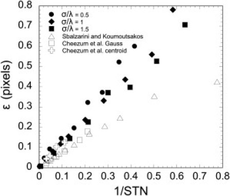
Standard deviation, ε, of the difference between particle position and speckle mark after refining with Gaussian-Fit, versus 1/S/N and ratio of point-spread function width to pixel size, σ/λ. Simulated particles were tracked as described in section S5 of the Supporting Material. The graphs shows data from Fig. 4 of Sbalzarini and Koumoutsakos (26) (σ/λ = 1) and Fig. 6 of Cheezum et al. (33) (σ/λ ≈ 1), who compared Gaussian-Fit and centroid algorithms. We did not include the lowest S/N data in Cheezum et al. (33) because some of these data points fall outside of the graph.

Below, we describe tests of our program, starting from simulated images of diffusing particles. We compare to other tracking tools in images of increasing complexity such as very high dynamic error and low S/N. We proceed to demonstrate the application of our method to experimental systems in which other free tools were unable to provide us with results due to additional complexities.

Single molecule diffusion simulations

A common task in particle tracking is measuring the diffusion coefficient, D. To validate and test the software, we generated simulated images of diffusing particles with different background noise levels (Fig. 2 A). We simulated point particles that perform random walks, contributing to the intensity of the image as they move during the exposure time, t_exp. The simulated camera exposure time was 50 ms and a pixel (px) represented 100 nm, similar to the experiments below. The time step dt = 0.0001 px²/(4 D) was adjusted such that the diffusion distance per dt is much less than a pixel. At each time step, particles were displaced by a distance selected from the two-dimensional diffusion propagator probability distribution. The intensity of each particle was convolved with a Gaussian kernel of standard deviation 2 px, representing the point-spread function.

Figure 2.

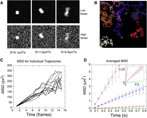
Tracking simulated diffusing particles. (A) Simulated images with increasing diffusion coefficients (left to right). (Bottom row) Same images with increased noise. (B) Marked trajectories. (C) MSD for individual tracks for D = 1 μm²/s (low noise). (D) Averaged MSD plots for different diffusion coefficients in Table 1. Error bars are mean ± 1 SD. (Inset) Enlarged version.

Further, we simulated the effects of camera noise, by adding normally distributed noise. We define the S/N ratio, S/N = I/σ_noise, where I is the average intensity (above the background) at the position of the speckle mark and σ_noise is the standard deviation of the intensity at the same position (26,33). These simulations did not include other sources of error such as fixed pattern noise, vibrations, drift, or fluctuations in the intensity of the fluorescent marker being tracked (3) (see Discussion).

In Fig. 2 A, slowly diffusing particles appear as small bright spots. With increasing D, diffusing particles appear as dimmer and more spread-out clouds due to diffusion during the exposure. This contributes to dynamic error (34,35). In addition, fast-moving particles move farther, so there are more crossed paths, which greatly hinders autotracking. The presence of noise especially limits the ability to detect clouds of fast-moving particles.

We tracked the particles in these images with our software and with two other software suites that have well-developed interfaces to handle complex tracking problems: Particle Tracker (26), which is based on the method developed by Crocker and Grier (15) and u-track (22). We tracked particles with our program using the Diffusing-Spots model and refined their positions using the Adjustment model followed by Gaussian-Fit (Fig. 2 B). To evaluate the accuracy, we measured the variance, s², of the distance between the speckle mark and the position of the simulated particle at the end of each exposure.

For low-diffusion coefficients, 0.01–0.1 μm²/s, all three particle trackers performed well, even at S/N below 4 (see Table 1). We were able to track the majority of the particles in the images through the end of the simulation (301 frames), with little need to fine-tune the program parameters (see Table S1 in Supporting Material). The calculated value of s² was consistent with the theoretical limit s² > 4/3 Dt_exp + 2ε², where ε is the static error in the absence of motion and 4/3 Dt_exp represents dynamic error (34). The calculated diffusion coefficients from plots of mean-square displacement (MSD) versus lag time achieved an accuracy >10% in most cases. These results suggest that our software is comparable to the existing tools under conditions that demand subpixel accuracy, where particles move on the order of ≤1 pixels per frame.

Table 1.

Results of tracking particles in simulated images using three different software tools

			u-track		Particle Tracker		Speckle TrackerJ
D (μm2/s)	S/N	4/3 D texp+2ε2 (px2)	s2 (px2)	D (μm2/s)	s2 (px2)	D (μm2/s)	s2 (px2)	D (μm2/s)
0.01	22.6	0.071	0.071 ± 0.0012	0.011	0.082 ± 0.0014	0.011	0.071 ± 0.0012	0.011
0.01	4.4	0.17	0.186 ± 0.003	0.011	0.266 ± 0.006	0.010	0.236 ± 0.004	0.011
0.1	20.4	0.67	0.68 ± 0.012	0.10	0.68 ± 0.011	0.11	0.68 ± 0.012	0.11
0.1	3.7	0.82	0.79 ± 0.013	0.11	0.85 ± 0.07	0.068	0.8 ± 0.013	0.10
1	6.3	6.8	6.9 ± 0.12	0.99	6.8 ± 0.12	1.0	6.9 ± 0.12	0.98
1	2.9	6.8	7.1 ± 0.13	1.01	7.5 ± 0.4	0.91	7.7 ± 0.13	1.0
4	3.4	27	33.8 ± 0.9	3.4	35.7 ± 2.0	4.3	36 ± 1.0	3.7
4	2.1	27	28 ± 1.1	3.5	∗	∗	47 ± 2.1	3.6

Columns 1 and 2 show simulated diffusion coefficient and S/N value. Column 3 shows the theoretical value for s², a sum of dynamic error and static error. Static error was calculated using the value of S/N and Fig. 1. The remaining columns show calculated s² and D.

^∗Unable to find good tracking parameters.

At the larger diffusion coefficients, 1 and 4 μm²/s, high dynamic error and low S/N makes tracking particles more challenging. Due to motion during exposure, the intensity of a particle can be so low that it is not discernable from the background.

For the high D cases, tuning the parameters in u-track and Particle Tracker leads to a tradeoff between broken tracks, due to missed particles, and many short-lived false positives (see Table 1 and Table S1). Although the performance can be optimized through tracking and linking parameters, manually pruning and merging tracks is not provided by the software. To address this issue, we limited our analysis to tracks that are longer than 20 frames. By doing this, we found the calculated diffusion coefficients were within 15% of the actual values. At high diffusion coefficients particles cross frequently, and during fully automated detection we could not exclude regions with clusters of particles. Some longer tracks were generated by switching from particle to particle.

An advantage of Speckle TrackerJ is the ability to track particles selectively. We were able to achieve the same accuracy in measuring high D values by seeding candidate speckle marks in regions with isolated particles and then Auto-Tracking. Even when Auto-Track failed after 10 frames, multiple tools allowed us to quickly find and manually join broken tracks and thus continue the track. For the highest noise and diffusion, both Speckle TrackerJ and u-track produced a similar number of total marks and a similar diffusion coefficient but the resulting tracks are quite different. Speckle TrackerJ yielded a few long tracks (see Table S1), which is an important aspect of particle tracking.

Each tracker required a similar amount of time to track particles. For problems that were tractable, the automated solutions for all three programs offered an advantage. For the more complicated scenarios, where it was impossible to automatically track all of the particles, Speckle TrackerJ quickly produced representative tracks. Selecting valid tracks is the main rate-limiting step in the analysis of the following experiments where a significant number of bright features such as clumps of immobile fluorophores need to be excluded from analysis.

Capping proteins at the leading edge of motile cells

Capping protein (CP) plays a critical role in regulation of actin-based structures, such as lamellipodial protrusions and actin patches in yeast (36,37). The α- and β-CP subunits bind to free barbed ends of actin filaments, blocking access to the barbed end. CP also interacts with phosphatidylinositol 4,5-bisphosphate (38). CP binding to membranes near the leading edge of motile cells may play a role in recruitment of CP protein to the leading edge (39,40). CP bound to the actin meshwork in lamellipodia dissociates from the network ∼25-fold faster than actin subunits (29). These findings suggested that cofilin-mediated actin filament severing triggers CP dissociation from the actin network by frequent severing. Fast severing and annealing reactions may contribute to structural reorganization of the actin network from the highly branched brushwork at the leading edge to the less branched network along the direction of retrograde flow (37).

To better understand why CP dissociates so fast in lamellipodia, we inspected diffuse CP, which would be separate from the actin network. We expect the diffusion coefficient of CP to represent the size of the protein, or protein complex to which they are attached. We performed experiments on XTC cells expressing EGFP-CPβ1 at low amounts and acquired images of the cell edge showing single CPs (Fig. 3, A and B). CP associated with the actin meshwork has a diffraction-limited spot appearance, whereas the faster diffusing species are more spread-out clouds (Fig. 3, A and B) similar to simulated images (Fig. 2 A).

Figure 3.

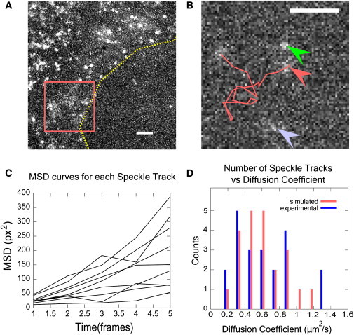
Tracking diffusing CPs at the leading edge of XTC cells. (A) Maximum intensity projection from a time-lapse recording of GFP-labeled CP at the leading edge. (Dashed line) Outline of leading edge. Exposure time was 66 ms and 1 pixel = 80 nm. Diffuse structures are diffusing molecules. (Bright speckles) CP proteins bound to the actin meshwork. (B) Enlarged section of box of panel A, single frame. (Line) Trace of a speckle track. (Middle arrow) Start of track. (Top arrow) Another diffusing speckle. (Bottom arrow) Cloud too mobile to track for enough frames. (C) MSD plots for individual speckle tracks from the time-lapse recording. (D) Distribution of diffusion coefficients found by fitting individual MSD curves with straight lines. Experimental: 22 tracked CPs. Simulated: results of tracking simulated particles for 10 frames with comparable conditions to the experiment: D = 0.6 μm²/s, 66 ms exposure, 1 px = 80 nm. Bin sizes are 0.14 μm²/s. Scale bars, 2 μm.

Tracking clouds of diffusing CP in Fig. 3 is challenging because of low S/N, high dynamic error, the presence of many static speckles and, occasionally, organelles that happen to contain fluorophores. The flexibility of our software allowed us to successfully track several of those diffusing molecules for 8–30 frames and calculate their individual MSD versus lag-time curves (Fig. 3 C). Fitting each MSD plot to a line, we calculated a distribution of diffusion coefficients, D (Fig. 3 D). The measured D values are in the range 0.2–2 μm²/s. Because we only tracked the CP speckles for as few as 10 frames, this range may represent measurement error: the accuracy in the measurement of D is lower when using shorter tracks. To evaluate this effect, we tracked particles in simulated images for 10 frames, with same exposure time and pixel size as in the experiment (41). Each particle had D = 0.6 μm²/s, and low noise was added to the image, same as in Fig. 2 A. We found a spread of D values similar to the spread of values in experiments (Fig. 3 D). We also note that the experimental images may include a population (we estimated ≤50%) of CP with D > 1 μm²/s that could not be tracked.

The D values in Fig. 3 D are much lower than those of proteins of similar molecular weight, e.g., actin monomers that are near 5 μm²/s (42). An intriguing hypothesis is that these slowly diffusing CPs are short severed actin filament oligomers. This would be consistent with the suggestion of Miyoshi et al. (29) that short CP lifetimes represent rapid actin filament severing near the barbed end. Future work is required, however, to test alternative mechanisms such as slow diffusion due to association of CP with the cell membrane.

Actin speckle lifetimes in lamellipodia

An important application of particle tracking involves measurements of lifetimes of actin monomers and tubulin dimers incorporated into filaments (11,13,29,43). When labeled actin or tubulin are in sufficiently low abundance compared to the unlabeled pool, polymerized labeled subunits appear as discrete speckles (Fig. 4 B) (11). Signals from diffusing subunits are much weaker because their intensity is distributed over several pixels (Fig. 2 A). Depending on the marker concentration, the speckles may represent single molecules (11,13,29,43) or groups of few labeled molecules (12,44). Single molecule speckle microscopy has shown that the dynamics of the cytoskeleton are characterized by continuous remodeling, involving constant assembly and disassembly that corresponds to speckle appearance and disappearance events in the images. Measurements of speckle lifetimes (time interval between speckle appearance and disappearance) have shown a broad distribution of lifetimes of actin in lamellipodia and tubulin in spindles (11,13,29). Tracking of speckle motions also provides information on filament transport (11–13,29,44).

Figure 4.

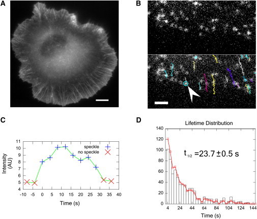
Speckle lifetime measurements. (A) XTC cell expressing EGFP-actin at high concentrations in which actin filaments in the lamellipodia appear as a continuous field. Scale: 8 μm. (B) Leading edge of lamellipodium with very dilute concentration of EGFP-actin. Single EGFP-actin monomers appear as speckles. (Bottom) Tracked speckles. Scale: 2.65 μm. (C) Intensity profile of speckle marked (arrow) in panel B. (D) Histogram of speckle lifetimes (n = 709). (Squares) Raw data. (Columns) Data normalized for photobleaching. Normalization and half-life estimation as in Watanabe and Mitchison (11).

We expressed EGFP-actin in XTC cells (11,29); see Fig. 4 A. We used cells with low EGFP-actin concentration (Fig. 4 B). In this panel, each speckle is a single actin monomer bound to the actin meshwork of the lamellipodium. During the course of the video (4 s intervals at 2 s exposure/frame), the actin speckles move away from the leading edge due to retrograde flow, as shown by the tracks in Fig. 4 B. Using the Constant-Velocity-NCC model, we tracked 900 actin speckles within 5 μm of the leading edge in 3–6 h, much faster compared to >12 h with the previous method (11). Each track was carefully checked: the automatic tracking still needed to be monitored to make sure of false-positives and speckle tracks that end prematurely due to gross changes in the background or blinking.

Fig. 4 C shows a typical graph of the intensity of a speckle through its lifetime. Measurements of speckle lifetimes demonstrate the rapid turnover of actin in the lamellipodium (Fig. 4 D). To calculate the half-life of actin monomers we adjusted the lifetimes to account for photobleaching and fit the cumulative number of speckles with an exponential (11). The measured half-life of 24 s is close to the previously measured value of 30 s (11).

SNARE-mediated fusion of single liposomes with supported bilayers, with single-molecule sensitivity

With few exceptions, intracellular fusion reactions are mediated by SNARE proteins; fusion is driven by pairing of vesicle-associated v-SNAREs with cognate t-SNAREs on the target membrane, resulting in a four-helix bundle (SNAREpin) that brings bilayers into close proximity (45,46). Much of our mechanistic understanding of SNARE-mediated fusion, as of this writing, has come from a bulk fluorescence dequenching assay in which small unilamellar vesicles containing v-SNAREs (v-SUVs) are mixed with SUVs containing t-SNAREs (t-SUVs) (45).

Recently, several researchers (47–50), including some of our group (32), have developed assays in which docking and fusion of single-vesicles with planar, supported bilayers (SBLs) can be detected. Unlike other single-vesicle approaches (47–50), this assay recapitulates the requirement for SNAP25, one of the essential t-SNARE components in vivo, without need for an artificial peptide (49). Using this assay, it was demonstrated previously that SUVs reconstituted with the synaptic/exocytic v-SNAREs VAMP/synaptobrevin fused rapidly with planar SBLs containing the synaptic/exocytic t-SNAREs syntaxin 1-SNAP25, with single fusion events occurring ∼130 ms after docking, and requiring 5–10 SNARE complexes per fusion event (32). Vesicles are continuously flown over the SBL. They dock at a constant rate and a small subset of docked vesicles fuse with the underlying SBL after a certain delay.

Diffusion of single fluorescent lipids from fused vesicles in supported bilayers

We used TIRFM to visualize for the first time, to our knowledge, the release and diffusion of single fluorescently labeled lipid molecules that initially reside in the SUV and become released into the SBL upon fusion of the two membranes. Because the SUV size is small (∼50 nm in diameter (32)), SUVs labeled with the fluorescent lipid LR-PE appear as diffraction-limited bright spots. After fusion, the LR-PE molecules diffuse away from the fusion site and become discernible as single speckles that can be tracked with ∼17ms time resolution (Fig. 5, A and B). Greater than 90% of the spots bleach in a single step, strongly suggesting they correspond to single-fluorophores.

Figure 5.

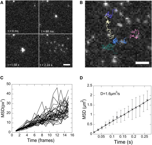
Single lipid tracking following vesicle fusion on a supported bilayer. (A) Montage of TIRFM images. (Top left) Before docking; (top right) docking; (bottom left) shortly after fusion; (bottom right) more time after fusion. Released lipids diffuse on the membrane. Residual lipids from prior fusion events can be seen in the first frame. (B) Image of tracked lipids. Images taken at 67 frames/s. (C) MSD for individual lipid trajectories. (D) Averaged MSD plots and linear fit from 33 lipids tracked for at least 30 frames. Error bars are 1 SD of the mean. Scale: 2.67 μm (10 pixels).

The challenge for tracking here is that the background at any time is filled with docked and unfused vesicles with a very broad range of intensities (due to different vesicle sizes and bleaching times), as well as with single molecules that have survived from other fusions. After visually identifying and seeding single molecules released from single fusion events, we tracked 33 single LR-PEs diffusing in the SBL that lasted >30 frames and calculated their MSD versus lag time (Fig. 5 C). The averaged MSD (Fig. 5 D) increases linearly with time, indicating a Brownian process. This suggests that the lipids that anchor the polymer cushion between the glass support and the SBL or membrane defects are dilute enough that they do not perturb LR-PE diffusion (51). We find D = 1.6 μm²/s, in close agreement with the diffusivity estimated previously from the increasing spread of the overall fluorescence signal as a function of time after fusion (32).

Analysis of vesicle docking and fusion events

Crucial information, only obtained by single-vesicle docking and fusion assays, is the lag time for fusion after a vesicle docks onto the SBL. This time reflects molecular mechanisms required for vesicles to become fusion-ready (e.g., by recruitment of proteins via lateral diffusion to the fusion site (32)) or rearrangements of the lipids/proteins leading to membrane fusion.

Docking of a vesicle onto the supported bilayer is characterized by the sudden appearance of a vesicle speckle, because TIRFM selectively visualizes only those vesicles very close to the surface (Fig. 6). In contrast, fusion events are characterized by the spread of the fluorescence intensity (initially concentrated within a SUV that appears as a diffraction-limited spot) within the SBL after merging of the SUV and SBL membranes.

Figure 6.

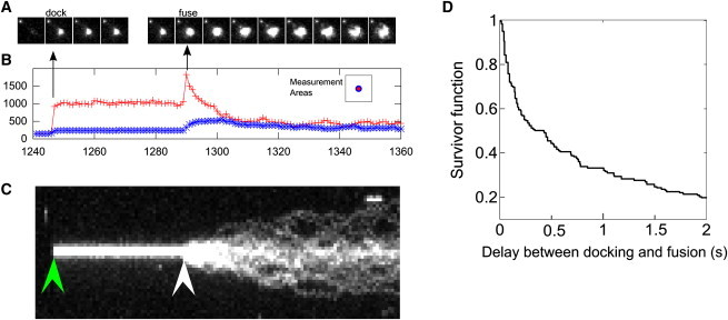
Detection and analysis of fusion events. (A) Successive frames of image sequence of a vesicle that docked (frame 1246) and fused (frame 1289). (B) Average intensities within an inner circle of 2.5 px radius centered at the position of the vesicle (top curve) and a surrounding ring 2.5 px wide (bottom curve). (C) The y-t projection of an image sequence. Docked vesicle appears as a thin band (left arrow). Fusion results in formation of comet-tail appearance (right arrow). (D) Probability that a vesicle survived without fusion beyond a given delay after docking (178 fusion events from 10 different acquisitions).

Measuring docking-to-fusion delays is challenging because: 1), The small subset of docked vesicles that fuse need to be identified; 2), broken trajectories and false detections distort the lifetime of the docked state; 3), docked vesicles have a broad intensity distribution; and 4), the vesicle disintegrates into numerous small speckles rapidly after fusion. Several algorithms have been designed for automated or lightly supervised detection of exocytosis events in live-cell TIRFM studies (10,52,53). These dedicated programs work well in specific applications, but are not completely reliable when conditions (cell type, marker properties, S/N) are changed. We have tested the program by Sebastian et al. (53) and a similar one written by one of us for SUV-SBL fusion, but have found that user input is required for the most reliable analysis of docking-to-fusion delays.

Two tools in Speckle TrackerJ assisted in identifying fusion events:

The first tool is based on tracing the intensities within a small circle around a vesicle and a ring just outside the circle. When fusion occurs, the average intensity in the inner circle initially increases sharply, within one frame: fluorophores come closer to the glass-buffer interface where the evanescent field intensity is higher, as well as due to polarization and possible dequenching effects (8,47,54). As the fluorophores leave the inner circle they enter the ring enclosing it. Thus, as the intensity in the inner circle drops, the intensity in the annulus increases (Fig. 6 B). This simple criterion was used in the past for assisting detection of fusion events (9).

The second tool is based on the projection of a sequence of images (xyt) onto the y-t plane. A docked vesicle appears as a bright line in such a projection, with the start of the line corresponding to the frame in which the vesicle docked. If the vesicle undocks, the line ends at the frame when undocking occurred. In contrast, if the vesicle fuses, then the dispersion of the fluorophores within the SBL results in a cometlike appearance of the projected profile (Fig. 6 C).

Fusing vesicles were identified as described above, and were tracked from the first frame in which they docked until the frame in which fusion occurred. A sample sequence is shown in Fig. 6 A. From these trajectories, we calculated the probability that a v-SUV survived beyond a delay t after docking (i.e., the survivor function; see Fig. 6 D). The delay time distribution matches closely the distribution obtained previously using mainly manual analysis (32).

Discussion

Speckle TrackerJ is most suited to situations where: 1), S/N is very low and/or particle mobility during camera exposure is high; 2), particles of interest constitute only a subset of all particles; 3), particle lifetimes in addition to mobilities are desired; and 4), particle densities are not too high so that the user supervision/assistance during tracking is feasible. The program can achieve subpixel resolution depending on the background noise and size of the pixel. Interpreting results that rely on subpixel resolution, however, requires careful consideration of additional issues, such as camera fixed pattern noise, vibration, shot noise, sample drift, and dynamic error. We refer the reader to extensive discussions in the literature on the relative importance of these factors and for recommendations on how to select experimental conditions for optimal tracking accuracy (3,4,18,34,35,55–58).

Tracking errors often lead to distorted MSD curves (3,18,34). The ability to control the quality of the acquired data in Speckle TrackerJ can help avoid possible artifacts due to the assumptions of tracking algorithms. Of course manual editing could also introduce errors: manual filling of gaps in particle tracks could distort the resulting MSD curves over the timescales related to the size of these gaps. Various tools in Speckle TrackerJ allow for easier testing and control of these issues.

There is a general trend toward fully automated, unsupervised detection, tracking, and analysis of larger and larger sets of data. However, at the forefront of single-molecule or single-vesicle biological research there are many situations where the S/N is very low, particle mobility is high during detection, a small subpopulation needs to be selectively analyzed, and/or both the particles and the background have broad intensity variations. Careful supervision of all tracks is required in such challenging situations, especially if the experimental approaches are new. The development of Speckle TrackerJ grew out of the need for a flexible tool combining supervised/assisted tracking with efficient automated algorithms. When imaging conditions are sufficiently good, Speckle TrackerJ allows unsupervised tracking with performance comparable to other, existing tools. In extremely difficult situations, with light user assistance, it allows obtaining and supervising tracks where existing tools fail.

References

- 1.Meijering E., Dzyubachyk O., van Cappellen W.A. Tracking in cell and developmental biology. Semin. Cell Dev. Biol. 2009;20:894–902. doi: 10.1016/j.semcdb.2009.07.004. [DOI] [PubMed] [Google Scholar]
- 2.Jaqaman K., Danuser G. Cold Spring Harbor Press; Cold Spring Harbor, NY: 2009. Computational Image Analysis of Cellular Dynamics: A Case Study Based on Particle Tracking. (This article can be found online, http://cshprotocols.cshlp.org/content/2009/12/pdb.top65.abstract). [DOI] [PMC free article] [PubMed] [Google Scholar]
- 3.Crocker J.C., Hoffman B.D. Multiple-particle tracking and two-point microrheology in cells. Methods Cell Biol. 2007;83:141–178. doi: 10.1016/S0091-679X(07)83007-X. [DOI] [PubMed] [Google Scholar]
- 4.Wirtz D. Particle-tracking microrheology of living cells: principles and applications. Annu. Rev. Biophys. 2009;38:301–326. doi: 10.1146/annurev.biophys.050708.133724. [DOI] [PubMed] [Google Scholar]
- 5.Brandenburg B., Zhuang X. Virus trafficking—learning from single-virus tracking. Nat. Rev. Microbiol. 2007;5:197–208. doi: 10.1038/nrmicro1615. [DOI] [PMC free article] [PubMed] [Google Scholar]
- 6.Dahan M., Lévi S., Triller A. Diffusion dynamics of glycine receptors revealed by single-quantum dot tracking. Science. 2003;302:442–445. doi: 10.1126/science.1088525. [DOI] [PubMed] [Google Scholar]
- 7.Karatekin E., Tran V.S., Henry J.P. A 20-nm step toward the cell membrane preceding exocytosis may correspond to docking of tethered granules. Biophys. J. 2008;94:2891–2905. doi: 10.1529/biophysj.107.116756. [DOI] [PMC free article] [PubMed] [Google Scholar]
- 8.Anantharam A., Onoa B., Axelrod D. Localized topological changes of the plasma membrane upon exocytosis visualized by polarized TIRFM. J. Cell Biol. 2010;188:415–428. doi: 10.1083/jcb.200908010. [DOI] [PMC free article] [PubMed] [Google Scholar]
- 9.Zenisek D., Steyer J.A., Almers W. Transport, capture and exocytosis of single synaptic vesicles at active zones. Nature. 2000;406:849–854. doi: 10.1038/35022500. [DOI] [PubMed] [Google Scholar]
- 10.Lopez J.A., Burchfield J.G., Hughes W.E. Identification of a distal GLUT4 trafficking event controlled by actin polymerization. Mol. Biol. Cell. 2009;20:3918–3929. doi: 10.1091/mbc.E09-03-0187. [DOI] [PMC free article] [PubMed] [Google Scholar]
- 11.Watanabe N., Mitchison T.J. Single-molecule speckle analysis of actin filament turnover in lamellipodia. Science. 2002;295:1083–1086. doi: 10.1126/science.1067470. [DOI] [PubMed] [Google Scholar]
- 12.Ponti A., Matov A., Danuser G. Periodic patterns of actin turnover in lamellipodia and lamellae of migrating epithelial cells analyzed by quantitative fluorescent speckle microscopy. Biophys. J. 2005;89:3456–3469. doi: 10.1529/biophysj.104.058701. [DOI] [PMC free article] [PubMed] [Google Scholar]
- 13.Needleman D.J., Groen A., Mitchison T. Fast microtubule dynamics in meiotic spindles measured by single molecule imaging: evidence that the spindle environment does not stabilize microtubules. Mol. Biol. Cell. 2010;21:323–333. doi: 10.1091/mbc.E09-09-0816. [DOI] [PMC free article] [PubMed] [Google Scholar]
- 14.Aratyn-Schaus Y., Oakes P.W., Gardel M.L. Dynamic and structural signatures of lamellar actomyosin force generation. Mol. Biol. Cell. 2011;22:1330–1339. doi: 10.1091/mbc.E10-11-0891. [DOI] [PMC free article] [PubMed] [Google Scholar]
- 15.Crocker J., Grier D.G. Methods of digital video microscopy for colloidal studies. J. Colloid Interface Sci. 1995;179:298–310. [Google Scholar]
- 16.http://physics.nyu.edu/grierlab/software.html.
- 17.http://www.physics.emory.edu/∼weeks/idl/.
- 18.Gao Y., Kilfoil M.L. Accurate detection and complete tracking of large populations of features in three dimensions. Opt. Express. 2009;17:4685–4704. doi: 10.1364/oe.17.004685. [DOI] [PubMed] [Google Scholar]
- 19.Rogers S.S., Waigh T.A., Lu J.R. Precise particle tracking against a complicated background: polynomial fitting with Gaussian weight. Phys. Biol. 2007;4:220–227. doi: 10.1088/1478-3975/4/3/008. [DOI] [PubMed] [Google Scholar]
- 20.Mashanov G.I., Molloy J.E. Automatic detection of single fluorophores in live cells. Biophys. J. 2007;92:2199–2211. doi: 10.1529/biophysj.106.081117. [DOI] [PMC free article] [PubMed] [Google Scholar]
- 21.http://www.nimr.mrc.ac.uk/gmimpro/.
- 22.Jaqaman K., Loerke D., Danuser G. Robust single-particle tracking in live-cell time-lapse sequences. Nat. Methods. 2008;5:695–702. doi: 10.1038/nmeth.1237. [DOI] [PMC free article] [PubMed] [Google Scholar]
- 23.Sergé A., Bertaux N., Marguet D. Dynamic multiple-target tracing to probe spatiotemporal cartography of cell membranes. Nat. Methods. 2008;5:687–694. doi: 10.1038/nmeth.1233. [DOI] [PubMed] [Google Scholar]
- 24.Matov A., Applegate K., Wittmann T. Analysis of microtubule dynamic instability using a plus-end growth marker. Nat. Methods. 2010;7:761–768. doi: 10.1038/nmeth.1493. [DOI] [PMC free article] [PubMed] [Google Scholar]
- 25.http://www.mosaic.ethz.ch/Downloads/ParticleTracker.
- 26.Sbalzarini I.F., Koumoutsakos P. Feature point tracking and trajectory analysis for video imaging in cell biology. J. Struct. Biol. 2005;151:182–195. doi: 10.1016/j.jsb.2005.06.002. [DOI] [PubMed] [Google Scholar]
- 27.http://www.imagescience.org/meijering/software/mtrackj/.
- 28.Sage D., Neumann F.R., Unser M. Automatic tracking of individual fluorescence particles: application to the study of chromosome dynamics. IEEE Trans. Image Process. 2005;14:1372–1383. doi: 10.1109/tip.2005.852787. [DOI] [PubMed] [Google Scholar]
- 29.Miyoshi T., Tsuji T., Watanabe N. Actin turnover-dependent fast dissociation of capping protein in the dendritic nucleation actin network: evidence of frequent filament severing. J. Cell Biol. 2006;175:947–955. doi: 10.1083/jcb.200604176. [DOI] [PMC free article] [PubMed] [Google Scholar]
- 30.Huet S., Karatekin E., Henry J.P. Analysis of transient behavior in complex trajectories: application to secretory vesicle dynamics. Biophys. J. 2006;91:3542–3559. doi: 10.1529/biophysj.105.080622. [DOI] [PMC free article] [PubMed] [Google Scholar]
- 31.http://athena.physics.lehigh.edu/speckletrackerj/.
- 32.Karatekin E., Di Giovanni J., Rothman J.E. A fast, single-vesicle fusion assay mimics physiological SNARE requirements. Proc. Natl. Acad. Sci. USA. 2010;107:3517–3521. doi: 10.1073/pnas.0914723107. [DOI] [PMC free article] [PubMed] [Google Scholar]
- 33.Cheezum M.K., Walker W.F., Guilford W.H. Quantitative comparison of algorithms for tracking single fluorescent particles. Biophys. J. 2001;81:2378–2388. doi: 10.1016/S0006-3495(01)75884-5. [DOI] [PMC free article] [PubMed] [Google Scholar]
- 34.Savin T., Doyle P.S. Static and dynamic errors in particle tracking microrheology. Biophys. J. 2005;88:623–638. doi: 10.1529/biophysj.104.042457. [DOI] [PMC free article] [PubMed] [Google Scholar]
- 35.Michalet X. Mean square displacement analysis of single-particle trajectories with localization error: Brownian motion in an isotropic medium. Phys. Rev. E. 2010;82:041914. doi: 10.1103/PhysRevE.82.041914. [DOI] [PMC free article] [PubMed] [Google Scholar]
- 36.Pollard T.D., Cooper J.A. Actin, a central player in cell shape and movement. Science. 2009;326:1208–1212. doi: 10.1126/science.1175862. [DOI] [PMC free article] [PubMed] [Google Scholar]
- 37.Watanabe N. Inside view of cell locomotion through single-molecule: fast F-/G-actin cycle and G-actin regulation of polymer restoration. Proc. Jpn. Acad. B Phys. Biol. Sci. 2010;86:62–83. doi: 10.2183/pjab.86.62. [DOI] [PMC free article] [PubMed] [Google Scholar]
- 38.Kim K., McCully M.E., Cooper J.A. Structure/function analysis of the interaction of phosphatidylinositol 4,5-bisphosphate with actin-capping protein: implications for how capping protein binds the actin filament. J. Biol. Chem. 2007;282:5871–5879. doi: 10.1074/jbc.M609850200. [DOI] [PMC free article] [PubMed] [Google Scholar]
- 39.Fujiwara I., Remmert K., Hammer J.A., 3rd Direct observation of the uncapping of capping protein-capped actin filaments by CARMIL homology domain 3. J. Biol. Chem. 2010;285:2707–2720. doi: 10.1074/jbc.M109.031203. [DOI] [PMC free article] [PubMed] [Google Scholar]
- 40.Kuhn J.R., Pollard T.D. Single molecule kinetic analysis of actin filament capping. Polyphosphoinositides do not dissociate capping proteins. J. Biol. Chem. 2007;282:28014–28024. doi: 10.1074/jbc.M705287200. [DOI] [PubMed] [Google Scholar]
- 41.Goulian M., Simon S.M. Tracking single proteins within cells. Biophys. J. 2000;79:2188–2198. doi: 10.1016/S0006-3495(00)76467-8. [DOI] [PMC free article] [PubMed] [Google Scholar]
- 42.McGrath J.L., Tardy Y., Hartwig J.H. Simultaneous measurements of actin filament turnover, filament fraction, and monomer diffusion in endothelial cells. Biophys. J. 1998;75:2070–2078. doi: 10.1016/S0006-3495(98)77649-0. [DOI] [PMC free article] [PubMed] [Google Scholar]
- 43.Yang G., Houghtaling B.R., Kapoor T.M. Architectural dynamics of the meiotic spindle revealed by single-fluorophore imaging. Nat. Cell Biol. 2007;9:1233–1242. doi: 10.1038/ncb1643. [DOI] [PubMed] [Google Scholar]
- 44.Danuser G., Waterman-Storer C.M. Quantitative fluorescent speckle microscopy of cytoskeleton dynamics. Annu. Rev. Biophys. Biomol. Struct. 2006;35:361–387. doi: 10.1146/annurev.biophys.35.040405.102114. [DOI] [PubMed] [Google Scholar]
- 45.Weber T., Zemelman B.V., Rothman J.E. SNAREpins: minimal machinery for membrane fusion. Cell. 1998;92:759–772. doi: 10.1016/s0092-8674(00)81404-x. [DOI] [PubMed] [Google Scholar]
- 46.Hu C., Ahmed M., Rothman J.E. Fusion of cells by flipped SNAREs. Science. 2003;300:1745–1749. doi: 10.1126/science.1084909. [DOI] [PubMed] [Google Scholar]
- 47.Liu T., Tucker W.C., Weisshaar J.C. SNARE-driven, 25-millisecond vesicle fusion in vitro. Biophys. J. 2005;89:2458–2472. doi: 10.1529/biophysj.105.062539. [DOI] [PMC free article] [PubMed] [Google Scholar]
- 48.Fix M., Melia T.J., Simon S.M. Imaging single membrane fusion events mediated by SNARE proteins. Proc. Natl. Acad. Sci. USA. 2004;101:7311–7316. doi: 10.1073/pnas.0401779101. [DOI] [PMC free article] [PubMed] [Google Scholar]
- 49.Domanska M.K., Kiessling V., Tamm L.K. Single vesicle millisecond fusion kinetics reveals number of SNARE complexes optimal for fast SNARE-mediated membrane fusion. J. Biol. Chem. 2009;284:32158–32166. doi: 10.1074/jbc.M109.047381. [DOI] [PMC free article] [PubMed] [Google Scholar]
- 50.Bowen M.E., Weninger K., Chu S. Single molecule observation of liposome-bilayer fusion thermally induced by soluble n-ethyl maleimide sensitive-factor attachment protein receptors (SNAREs) Biophys. J. 2004;87:3569–3584. doi: 10.1529/biophysj.104.048637. [DOI] [PMC free article] [PubMed] [Google Scholar]
- 51.Deverall M.A., Garg S., Naumann C.A. Transbilayer coupling of obstructed lipid diffusion in polymer-tethered phospholipid bilayers. Soft Matter. 2008;4:1899–1908. [Google Scholar]
- 52.Mele, K., A. Coster, …, P. Valotton. 2009. Automatic identification of fusion events in TIRF microscopy image sequences. In Computer Vision Workshops (ICCV Workshops), 2009 IEEE 12th International Conference on Kyoto. 578–584.
- 53.Sebastian R., Diaz M.E., Toomre D. Spatio-temporal analysis of constitutive exocytosis in epithelial cells. IEEE/ACM Trans. Comput. Biol. Bioinform. 2006;3:17–32. doi: 10.1109/TCBB.2006.11. [DOI] [PubMed] [Google Scholar]
- 54.Axelrod D., Burghardt T.P., Thompson N.L. Total internal reflection fluorescence. Annu. Rev. Biophys. Bioeng. 1984;13:247–268. doi: 10.1146/annurev.bb.13.060184.001335. [DOI] [PubMed] [Google Scholar]
- 55.Thompson R.E., Larson D.R., Webb W.W. Precise nanometer localization analysis for individual fluorescent probes. Biophys. J. 2002;82:2775–2783. doi: 10.1016/S0006-3495(02)75618-X. [DOI] [PMC free article] [PubMed] [Google Scholar]
- 56.Wu P.H., Agarwal A., Tseng Y. Analysis of video-based microscopic particle trajectories using Kalman filtering. Biophys. J. 2010;98:2822–2830. doi: 10.1016/j.bpj.2010.03.020. [DOI] [PMC free article] [PubMed] [Google Scholar]
- 57.Wu P.H., Arce S.H., Tseng Y. A novel approach to high accuracy of video-based microrheology. Biophys. J. 2009;96:5103–5111. doi: 10.1016/j.bpj.2009.03.029. [DOI] [PMC free article] [PubMed] [Google Scholar]
- 58.Berglund A.J. Statistics of camera-based single-particle tracking. Phys. Rev. E. 2010;82:011917. doi: 10.1103/PhysRevE.82.011917. [DOI] [PubMed] [Google Scholar]
Associated Data
This section collects any data citations, data availability statements, or supplementary materials included in this article.