Comparison of Penalty Functions for Sparse Canonical Correlation Analysis

Abstract

Canonical correlation analysis (CCA) is a widely used multivariate method for assessing the association between two sets of variables. However, when the number of variables far exceeds the number of subjects, such in the case of large-scale genomic studies, the traditional CCA method is not appropriate. In addition, when the variables are highly correlated the sample covariance matrices become unstable or undefined. To overcome these two issues, sparse canonical correlation analysis (SCCA) for multiple data sets has been proposed using a Lasso type of penalty. However, these methods do not have direct control over sparsity of solution. An additional step that uses Bayesian Information Criterion (BIC) has also been suggested to further filter out unimportant features. In this paper, a comparison of four penalty functions (Lasso, Elastic-net, SCAD and Hard-threshold) for SCCA with and without the BIC filtering step have been carried out using both real and simulated genotypic and mRNA expression data. This study indicates that the SCAD penalty with BIC filter would be a preferable penalty function for application of SCCA to genomic data.

1. Introduction

Few statistical methods have been developed to maximize the use of the enormous amount of genomic data to unravel the etiology of complex disease and drug related phenotypes. Currently, the standard analysis method for large genome-scale data has concentrated on analysis of a single data type, or experiment, at a time. This analysis approach ignores the interaction between genes, proteins and biochemical reactions which give rise to complex diseases and drug related phenotypes. Therefore, integrative analytical approaches are needed for the simultaneous assessment of multiple genomic data types and their influence on drug related-phenotypes and complex diseases.

One approach for such integrative analysis is canonical correlation analysis (CCA), proposed by Hotelling (1936). CCA focuses on the correlation between a weighted linear combination of variables in one set and a weighted linear combination of the variables in another set. The objective of CCA is to identify the pair of linear combinations having maximum correlation. The pairs of linear combinations are referred to as the canonical variables and their correlations are called canonical correlations. Following the identification of the first canonical correlation and canonical variables, the second pair of linear combinations is identified among all pairs uncorrelated with the initially selected pair, and so on. However, in many situations, attention is focused primarily on the first canonical correlation and variables.

When the number of variables far exceeds the number of subjects, such as in case of large-scale genomic studies, traditional CCA methods are no longer appropriate. In addition, when the variables are highly correlated, sample covariance matrices become unstable or undefined, leading to additional difficulty in estimating the canonical correlation and variables. Therefore, classical CCA requires a dimension reduction method to overcome this problem. Numerous methods have been developed for shrinkage and variable selection over the past decade including least absolute shrinkage and selection operator (Lasso) by Tibshirani (1996), Elastic-net by Zou and Hastie (2005), Smoothly Clipped Absolute Deviation (SCAD) by Fan and Li (2001) and non-negative Garrote by Breiman (1995). Recently, these methods have been applied to CCA for assessing the relationships between two sets of high-dimensional genomic data. The variable selection techniques are applied to the canonical variable loadings which set some of the coefficients to exact zeros, thereby selecting the remaining variables. The important variables selected are then called the sparse set of variables and the canonical correlation analysis using these variables is often referred to as sparse canonical correlation analysis (SCCA). Waaijenborg et al. (2008) first suggested a penalized version of canonical correlation analysis using an iterative regression procedure with the Univariate Soft Threshold (UST) version of the Elastic-net penalty. Subsequently, Parkhomenko et al. (2009) suggested the SCCA method using a form of regularization similar to UST elastic-net (Zou and Hastie, 2005). Witten et al. (2009) used the Lasso penalty in their SCCA. These methods are appealing; however, they do not directly control the sparsity of the solution. As a result, the methods may not necessarily produce sparse set of variables (Lykou and Whittaker, 2009). To overcome the issue, Zhou and He (2008) suggested two-step-procedure in carrying out SCCA in which a L₁ penalty was used on the variable loadings during the first step followed by additional variable filtering algorithm that uses Bayesian Information Criterion (BIC). However, no assessment to determine the “optimal” penalty function for SCCA involving genomic data has been completed.

In this paper, the performances of various penalty functions are assessed in application to SCCA, using the SCCA algorithm as outlined by Parkhomenko et al. Four penalty functions including Lasso (Tibshirani, 1996), Elastic-net (Zou and Hastie, 2005), SCAD (Fan and Li, 2001) and Hard-thresholding (Antoniadis, 1997) were applied to a pharmacogenomics study of the drug gemcitabine, along with simulation studies to assess the performance of the penalty functions to SCCA. In addition, the BIC variable filtering method was used, as outlined by Zhou and He (2008), to further filter out unimportant variables. Results from the simulation study indicate that the SCAD penalty with a BIC filter is a preferable penalty to use in the SCCA for genomic data.

2. Methods and Materials

2.1. Sparse canonical correlation analysis (SCCA)

Canonical correlation analysis (CCA) is a multivariate statistical method designed to explore the correlation between two sets of quantitative variables (Hotelling, 1936). Suppose two data sets X = (X¹, X²,…, X^p) and Y = (Y¹, Y²,…,Y^q) are of dimensions n × p and n × q, with p ≤ n and q ≤ n measured on the same set of n subjects. Suppose the columns of X and Y are standardized to have mean zero and standard deviation one. Let u and v be p×1 and q×1 vectors of weights and let ξ = Xu and η = Yv be linear combinations of the variables in data sets X and Y respectively, where ξ and η are n×1 vectors. Then, the coefficient vectors u and v are estimated by maximizing the following equation,

$$\begin{array}{l}\rho =\frac{\mathit{Cov}(\mathbf{\xi },\mathbf{\eta })}{{[\mathit{Var}(\mathbf{\xi })\mathit{Var}(\mathbf{\eta })]}^{1/2}}\\ =\frac{{\mathbf{u}}^{\mathbf{T}}{\mathbf{X}}^{\mathbf{T}}\mathbf{Yv}}{{[({\mathbf{u}}^{\mathbf{T}}{\mathbf{X}}^{\mathbf{T}}\mathbf{Xu})({\mathbf{v}}^{\mathbf{T}}{\mathbf{Y}}^{\mathbf{T}}\mathbf{Yv})]}^{1/2}},\end{array}$$ (1)

where X^TX and Y^TY are within-data covariance matrices and X^TY is the between-data covariance matrix. Note that scaling u and v does not affect the correlation coefficient. Therefore, the above equation can be re-expressed in the following way:

$$\rho =\mathit{corr}(\mathbf{\xi },\mathbf{\eta })=max{\mathbf{u}}^{\mathbf{T}}{\mathbf{X}}^{\mathbf{T}}\mathbf{Yv}\text{subject}\text{to}{\mathbf{u}}^{\mathbf{T}}{\mathbf{X}}^{\mathbf{T}}\mathbf{Xu}={\mathbf{v}}^{\mathbf{T}}{\mathbf{Y}}^{\mathbf{T}}\mathbf{Yv}=1.$$ (2)

When the number of variables is larger than the sample size, the CCA method mentioned above is not applicable. Possible multicollinearity between predictor variables further adds difficulty in the computation because the covariance matrices can become unstable or undefined. Therefore, a few important variables are selected using standard model selection criteria and the canonical correlation is computed using the selected set of variables making the results interpretable, which is referred to as Sparse Canonical Correlation Analysis (SCCA). Mathematically, SCCA is computed by maximizing the following penalized objective function, $\rho =\mathit{corr}(\mathbf{\xi },\mathbf{\eta })=\underset{u,v}{max}{\mathbf{u}}^{\mathbf{T}}{\mathbf{X}}^{\mathbf{T}}\mathbf{Yv}$ subject to, u^TX^TXu = v^TY^TYv= 1 with Penalties P ₁(u) and P ₂(v) on u and v respectively.

To deal with the multicollinearity issue, several methods have been proposed. Vinod (1976) proposed adding penalty terms to the diagonal elements of the covariance matrix which is similar to the ridge regression concept in regression analysis. This requires estimation of additional ridge parameters. Other extreme types of regularization have been used where the variance matrices are replaced with their corresponding diagonal matrices (Parkhomenko 2009) or identity matrices (Witten 2009). In this paper, the matrices X^TX and Y^TY are replaced with their corresponding diagonal matrices similar to the approach proposed by Parkhomenko et al. (2009).

2.2. Regularization and Shrinkage methods

Penalized linear regression techniques have been widely used to analyze high dimensional data which have in-built shrinkage and variable selection mechanisms. Let y be a n×1 vector and X be a n × p matrix. Then the penalized regression coefficient β is estimated from the following penalized regression model:

$${\widehat{\beta }}^{\mathit{penalized}}=\underset{\beta }{argmax}{\mid y-X\beta \mid }^2+p_{\lambda }(\beta ),$$ (3)

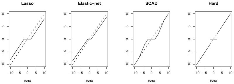
where p_λ (β) is the penalty term and λ is a tuning parameter which is estimated using cross validation or permutation methods. Ridge regression (Hoerl and Kennard, 1970) was the first penalized regression method designed to mediate the multicollinearity among the predictors in which a quadratic penalty term is added to the regular least square estimating equations. Ridge regression shrinks the coefficients towards zero by imposing a penalty on their squared size; however the shrunken coefficients never equal zero. As a result, ridge regression does not perform variable selection. Other penalty functions, such as Lasso, Elastic-net and SCAD, are available which account for the multi-collinearity issue (“shrinkage”) as well as set some of the coefficients to exact zeros producing sparse set of variables (i.e., variable selection). In this paper, we compare the performances of various penalty functions for SCCA using the algorithm as outlined by Parkhomenko et al. (2009). For all penalty functions, the sparseness parameters (tuning parameters for the penalty function) are estimated using cross validation. Figure 1 shows the thresholding rules or the solution functions of the four penalty functions assessed in this paper.

Figure 1.

Plots showing the thresholding rules of the four penalty functions.

2.2.1. Lasso penalty

The least absolute shrinkage and selection operator (Lasso) is a shrinkage method which sets some of the coefficients to zero and hence retains the ability of selecting important features (Tibshirani, 1996). The Lasso penalty term is defined as, $p_{\lambda }^{\mathit{lasso}}(\beta )=\lambda {\displaystyle \sum _{j=1}^p}\mid {\beta }_j\mid$, where λ is a tuning parameter. The solution of Lasso regression can be given as

$${\widehat{\beta }}_j^{\mathit{lasso}}={(\mid {\widehat{\beta }}_j\mid -\lambda )}_{+}\mathit{sign}({\widehat{\beta }}_j)$$ (4)

This coincides with the soft thresholding rule proposed by Donoho and Johnstone, (1994) and Donoho et al. (1995) which was applied to wavelet coefficients for the estimation of a function. SCCA utilizes a similar soft thresholding operator on the variable loading u and v, as û_j =(|û_j|−λ₁)₊ sign (û_j) and v̂_j =(|v̂_j|−λ₂)₊ sign (v̂_j) respectively.

2.2.2 Elastic-net penalty

Elastic-net (Zou and Hastie, 2005) is a regularization technique that simultaneously performs variable selection and continuous shrinkage. This method uses both the L₂ quadratic penalty of ridge regression and the L₁ penalty of Lasso, forming a convex combination. Therefore, this method retains the variable selection property while correcting for the extra shrinkage. The elastic net penalty function can be defined as $p_{\lambda }^{\mathit{elastic}-\mathit{net}}(\beta )={\lambda }_1{\displaystyle \sum _{j=1}^p}\mid {\beta }_j\mid +{\lambda }_2{\displaystyle \sum _{j=1}^p}{\beta }_j^2$. However, the computational cost is slightly higher for Elastic-net, as two tuning parameters need to be estimated.

As an alternative to Elastic-net, Zou and Hastie (2005) proposed univariate soft thresholding (UST) as a simplified version of the elastic-net; the solution of which is given as,

$${\widehat{\beta }}_j^{\mathit{elastic}-\mathit{net}}={(\mid {\widehat{\beta }}_j\mid -0.5\lambda )}_{+}\mathit{sign}({\widehat{\beta }}_j).$$ (5)

SCCA methods proposed by Waijenborg et al. (2008) and Parkhomenko et al. (2009) both use a soft thresholding rule similar to UST. In this paper, the univariate soft threshold version of the Elastic-net is used on variable loadings u and v as follows and is referred it as Elastic-net type of penalty: û_j =(|û_j|−0.5λ₁)₊ sign (û_j) and v̂_j =(|v̂_j|−0.5 λ₂)₊ sign (v̂_j).

2.2.3. Smoothly clipped absolute deviation penalty (SCAD)

Fan and Li (2001) proposed a non-convex penalty function referred to as the smoothly clipped absolute deviation (SCAD). They provided the following three criteria for a good penalty function: (i) Unbiasedness, (ii) Sparsity and (iii) Continuity. They further argued that SCAD penalty satisfies these properties. The SCAD penalty is given by

$$p_{\lambda }^{\mathit{scad}}(\beta )=\{\begin{array}{ll}\lambda \mid {\beta }_j\mid \hfill & \text{if}\mid {\beta }_j\mid \le \lambda \hfill \\ -\left(\frac{{\mid {\beta }_j\mid }^2-2a\lambda \mid {\beta }_j\mid +{\lambda }^2}{2(a-1)}\right)\hfill & \text{if}\lambda <\mid {\beta }_j\mid \le a\lambda \hfill \\ \frac{(a+1){\lambda }^2}{2}\hfill & \text{if}\mid {\beta }_j\mid >a\lambda \hfill \end{array}.$$ (6)

This corresponds to a quadratic spline function with knots at λ and aλ. The function is continuous and the first derivative for some a>2 and β> 0 can be given by

$$p_{\lambda }^{\prime }(\beta )=\lambda \left\{I(\beta \le \lambda )+\frac{{(a\lambda -\beta )}_{+}}{(a-1)\lambda }I(\beta >\lambda )\right\}.$$ (7)

The SCAD penalty is continuously differentiable on (−∞, 0)∪(0,∞) but singular at 0 with its derivatives zero outside the range[−aλ, aλ]. This penalty function results in small coefficients being set to zero, mid-size coefficients being shrunk towards zero and large coefficients remaining untouched. Thus, SCAD penalty produces a sparse solution and approximately unbiased coefficients for large coefficients. The solution for the SCAD penalty can be given as

$${\widehat{\beta }}_j^{\mathit{SCAD}}=\{\begin{array}{ll}{(\mid {\widehat{\beta }}_j\mid -\lambda )}_{+}\mathit{sign}({\widehat{\beta }}_j)\hfill & \hfill \text{if}\mid {\widehat{\beta }}_j\mid \le 2\lambda \\ \left\{(a-1){\widehat{\beta }}_j-\mathit{sign}({\widehat{\beta }}_j)a\lambda \right\}/(a-2)\hfill & \hfill \text{if}2\lambda <\mid {\widehat{\beta }}_j\mid \le a\lambda \\ {\widehat{\beta }}_j\hfill & \hfill \text{if}\mid {\widehat{\beta }}_{\text{j}}\mid >a\lambda \end{array}$$ (8)

This thresholding rule involves two unknown parameters λ and a. Theoretically, the best pair (λ, a) can be obtained using a two dimensional grid-search with criteria similar to cross validation methods. However, such an implementation could be computationally expensive. Based on a Bayesian standpoint and simulation studies, Fan and Li (2001) suggested a =3.7 to be a good choice for various problems. They have further argued that the performance of various variable selection problems do not improve significantly with a selected by data driven methods. In our comparison of the penalty functions, a was set to 3.7 with λ selected by cross validation. As mentioned before, the thresholding rule (8) was used for loading vectors u and v in this paper.

2.2.4. Hard-threshold penalty

Hard-thresholding, due to Antoniadis (1997) and Fan (1997), sets some coefficients to zero directly. But since it does not shrink any coefficients towards zero, this penalty function does not solve the problem of multicollinearity among the predictors. However, this penalty results in unbiased estimates for the variables with large effects. The solution of the hard-thresholding rule is given by

$${\widehat{\beta }}_j^{\mathit{hard}}={\beta }_{j}I(\mid {\beta }_j\mid >\lambda ).$$ (9)

2.3. Selection of sparseness parameters

Waaijenborg et al. (2008) and Parkhomenko et al. (2009) recommend k-fold cross validation method to optimize the penalty parameters for each canonical variate pair. The data is divided into two parts: $\frac{k-1}{k}$ proportion of data for training and the remaining $\frac{1}{k}$ proportion of data for testing (validation). The loading vectors are estimated in the training set and applied to the testing set. Parkhomenko et al. (2009) use cross validation to select the sparseness parameters λ_u and λ_v by maximizing the test sample correlation. The weight vectors u and v are estimated using the pre-specified values of λ_u andλ_v. Then, the correlation is computed as,

$${\mathrm{\Delta }}_{\mathit{cor}}=\frac{1}{k}\sum _{j=1}^k\left|\mathit{cor}({\mathbf{X}}_{\mathbf{j}}{\mathbf{u}}^{-\mathbf{j}},{\mathbf{Y}}_{\mathbf{j}}{\mathbf{v}}^{-\mathbf{j}})\right|,$$ (10)

where k is number of times the cross validation is performed, u^−j and v^−j are the weight vectors in the training sets X_−j and Y_−j respectively, in which the subset j was removed. Similarly, X_j and Y_j are the test sets respectively. Then λ_u and λ_v values corresponding to the maximum value of Δ_cor are the optimum sparseness (tuning) parameters.

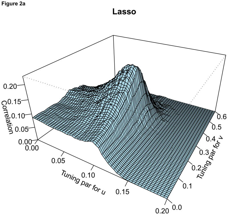
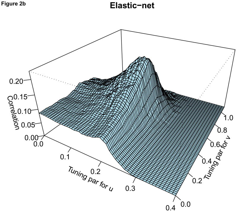
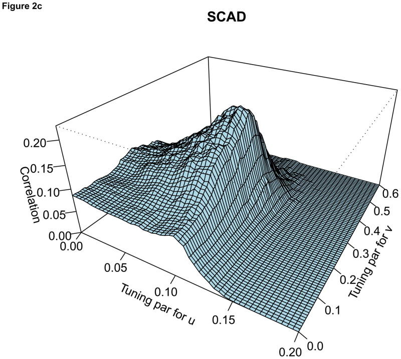
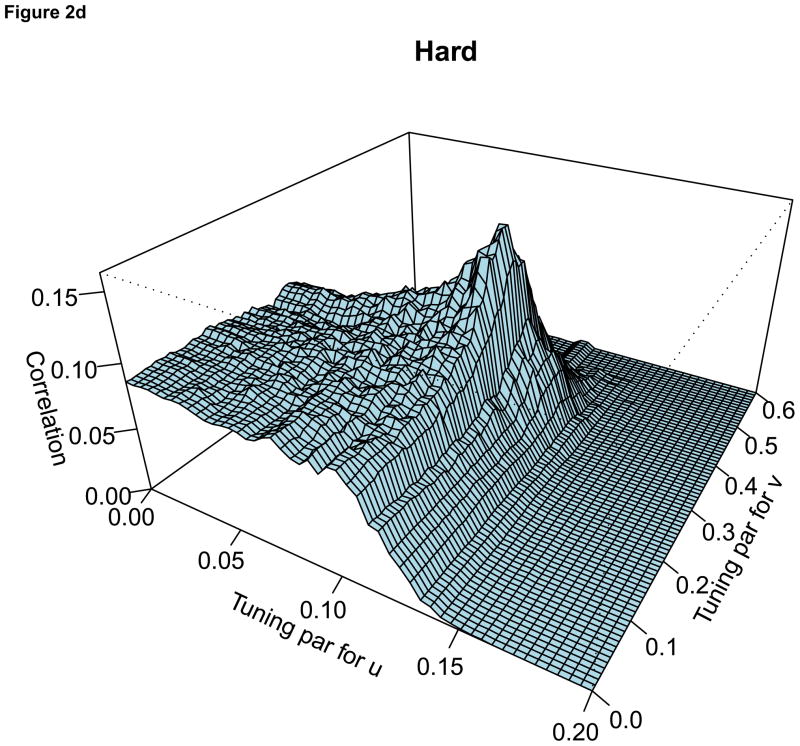
For the comparison of the penalty functions, in this paper, the approach of Parkhomenko et al. (2009) was used to select the tuning parameters. Sample 3D plots of test sample correlation vs tuning parameters are shown in Figure 2, with λ_u, λ_v and correlation coefficients on the X-axis, Y-axis and Z-axis respectively. The peaks in each plot correspond to maximum test sample correlation and combination of tuning parameters.

Figure 2.

For each plot, the X-axis represents the tuning parameter for u, Y-axis represents the tuning parameter for v and Z-axis represents the test sample correlation. Each plot represents sample plot for one simulated data only. Each simulated data has its own tuning parameters and the test sample correlation.

2.5. Variable filtering using BIC information

The main disadvantage of the available SCCA methods is that they do not have direct control over the sparsity. As a result, it is difficult to achieve effective dimension reduction. There is a trade-off between the maximum correlation and the sparsity of the variables. Zhou and He (2008) proposed two-step procedure balancing the loss in the correlation and gain in the sparsity of variables. In first step, they set a constraint on the loadings such that the sparse-correlation does not decrease below a lower confidence limit of the approximated canonical correlation by gradually imposing constraint through an iterative procedure. In the second step, the variable filtering is carried out using a BIC-type criterion, setting the smallest loading in absolute value to zero at each iteration for both variables. The new correlation coefficient is computed corresponding to new loadings at each iteration and the BIC is estimated by using

$$\mathit{BIC}(d)=nlog(1-r_d^2)+dlog(n),$$ (11)

where d =p+q is total number of parameters, n is sample size and $r_d^2$ is the correlation coefficient with d parameters. The variables corresponding to the minimum BIC value are the final selected variables.

2.6. Description of the Human Variation Panel

SCCA, using the various penalty functions, was applied to data collected on the HVP (Human Variation Panel). The HVP consists of EBV-transformed lymphoblastoid cells derived from 51 Caucasian-American (CA), 45 African-American (AA) and 51 Han Chinese-American (HCA) subjects (Coriell Institute, Camden, NJ) resulting in a total sample size of 147. Whole genome Expression data for the HVP was obtained using Affymetrix U133 Plus 2.0 Expression array chips, containing over 54,000 probe sets (Li et al., 2008). The mRNA Expression array data were normalized on the log2 scale using the GCRMA methodology (Zhijin et al., 2004). The gemcitabine pathway contains 31 probe sets from the Affymetrix U133 plus 2.0 Expression array chip.

Gnome-wide single nucleotide polymorphism (SNP) data was obtained using Illumina HumanHap 550K BeadChips for the HVP. The SNP genotyping was completed at the Genotyping Shared Resources at the Mayo Clinic in Rochester, MN (Li et al., 2009). SNPs mapped to the gemcitabine pathway, which passed quality control, were identified. In particular, there are 19 genes in the pathway with a total of 749 SNPs that meet Hardy-Weinberg equilibrium (HWE p > 0.001) and call rate > 95%. Missing genotypes were imputed prior to all analyses using the program fastPHASE (Scheet and Stephens, 2006). In this paper, the performances of the various penalty functions for SCCA are compared using the 31 mRNA Expression probe sets and 749 SNPs in the 19 genes within the gemcitabine pathway from the HVP.

SNP data from the HVP for the gemcitabine pathway was adjusted for race and possible population stratification as outlined by Niu et al. (2010). A principal component analysis (PCA) approach was used to adjust for population stratification, in which PCA was completed by race with the top five principal components saved. Individual genotypes were regressed on race and race specific principal components to obtain the residuals. The mRNA expression data was adjusted similarly for gender, race and population stratification. Then SCCA was applied to the adjusted data using the four different penalty functions.

2.7. Description of the simulated data

Simulation of the genotype data was based on the gemcitabine pathway SNP data, for the Caucasian cell lines within the HVP. Genotypes within genes in the gemcitabine pathway were mapped to chromosomes, with haplotype phase inferred from the SNP genotypes on the same chromosome using the program fastPHASE (Scheet and Stephens, 2006). These haplotype frequencies were used as the “true” haplotype frequencies for the underlying population, with haplotypes simulated using the hapsim library in R (http://cran.r-project.org/web/packages/hapsim/index.html). These haplotypes were then assigned in a sequential fashion to the 200 individuals, producing simulated genotypes for SNPs within the gene (and thus pathway) that mimic realistic LD for markers within the same gene, in addition to LD between genes on the same chromosome.

Following the simulation of the genotype data for n=200 subjects, mRNA gene expression data was simulated, such that, some of the SNPs were correlated with some of the mRNA variables. The mRNA expression values for each individual were simulated using a multivariate normal distribution X= M V N (μ_i, Σ), where μ_i = G_i × B, the mean for individual i, is based on the effect matrix B and genotypes for each individual G_i.Matrix B and vector G_i are defined in the following way. Let

$$\mathbf{B}=\left(\begin{array}{cccc}k& 0& \dots & 0\\ 0& 0& \dots & k\\ \dots & \dots & \dots & \dots \\ 0& 0& k& 0\end{array}\right)$$

represent a matrix with the number of rows equal to the number of SNPs and number of columns equal to the number of mRNA variables (i.e., B is a 734 by 31 matrix). Next, SNPs were selected to be associated with gene expression, with effect size of k = 0.96 for those SNP-mRNA pairs. Using this mean μ_i (based on G_i and B) and covariance matrix (Σ) based on the observed correlation structure between the mRNA expression values within the gemcitabine pathway, mRNA data for individual i was simulated. In addition, the simulations were also run with sample sizes 100, 150, 250, 300, 350, 400, 450 and 500 to assess the effects of the sample sizes on the performance of the methods. One-hundred simulations were run for each sample size.

3. Results

3.1 SCCA of the HVP data

Table 1 displays the sparse canonical correlations and the number of variables selected using various penalty functions when applied to the gemcitabine pathway. SCAD selected the fewest SNPs (113) and mRNA variables (21). Lasso, Elastic-net, and Hard-thresholding selected 316, 257 and 320 SNPs out of 749 total SNPs and 28, 26 and 27 mRNA expression variables out of 31 genes, respectively. The correlation coefficients from Lasso, Elastic-net and Hard-threshold were similar (r around 0.67); however, the correlation coefficient from the SCAD method (r =0.6059) was the smallest out of the four penalties.

Table 1.

Sparse canonical correlations and number of selected variables before and after using BIC filter method for the genomic data from the HVP.

Penalty	Before using BIC			After Using BIC
	Correlation (ρ)	SNP	mRNA	Correlation (ρ)	SNP	mRNA
Lasso	0.6657	316	28	0.4733	5	5
Elastic Net	0.6762	257	26	0.4849	6	5
SCAD	0.6059	113	21	0.4367	4	2
Hard-threshold	0.6605	320	27	0.5123	9	5

Next, the overlap of the selected variables for the four penalty functions was assessed, with 107 SNPs and 19 mRNA variables selected by all penalty functions. In addition to these commonly selected variables, 1 SNP and 1 mRNA was selected exclusively by Lasso, 1 SNP was only selected by Elastic-net, 5 SNPs and 1 mRNA were only selected by SCAD and 5 SNPs were only selected by Hard-threshold. Considering the two-way overlap of selected SNPs, there were 58 SNPs present only in Lasso and Hard-threshold, with no two-way over lap for mRNA variables. For three-way overlaps of selected variables, 149 SNPs and 7 mRNA variables were selected for Lasso, Elastic-Net and Hard-threshold with 1 SNP and 1 mRNA expression overlap for Lasso, SCAD and Hard-threshold. These results show that, except for a few cases, all four penalty functions selected a common set of variables.

However, SCCA with all four penalty functions resulted in a large number of selected variables. Following the application of the BIC filter, Lasso, Elastic-net, SCAD and Hard-thresholding selected 5, 6, 4 and 9 SNPs and 5, 5, 2 and 5 mRNA variables, respectively. As there is reduction in the number of variables, the corresponding first canonical correlation values were also reduced (values for r ranged from 0.43 to 0.51). There were 3 SNPs (rs10742250, rs17103186 and rs4877848) and 2 mRNA (201802_at and 1553995_a_at) variables selected by all four penalty functions. The fourth SNP selected by SCAD (rs1474500) was also selected by Elastic-net. There were 3 SNPs (rs10251079, rs10835678 and rs1332535) selected only by the Hard-threshold penalty.

3.2 SCCA of the simulated data

In addition to the application of SCCA using the four penalty functions to the HVP, the methods were also applied to simulated data sets, in which the “truth” was known. Seven SNP variables (rs2840075, rs16961564, rs1246274, rs2778944, rs7776847, rs11776754 and rs1265147) and five mRNA variables (203302_at, 219708_at, 220475_at, 223298_s_at and 223342_at) were chosen to have “non-zero” effects. The results were compared with respect to three parameters: average number of false discoveries (AvgFD); average number of non-discoveries (AvgND); and number of times true variables were selected (NTTS). False discovery here is defined as the number of noise variables selected and non-discovery represents the number of true variables that were not selected. AvgFD was computed by adding all the false discoveries detected across 100 simulations divided by 100 and AvgND was computed by adding all the non-discoveries across 100 simulations divided by 100. NTTS was computed for each true variable by keeping track of the number of simulations (out of 100) in which significant effects were detected. For example, if SNP rs2840075 was detected in 74 simulations out of 100 simulations, then the NTTS value for rs2840075 is 74. The NTTS values for both SNPs and mRNA were generally higher for the SCAD penalty. Therefore, to facilitate the comparison, the observed NTTS values for variables from Lasso, Elastic-net and Hard threshold were re-scaled with respect to the NTTS values of those variables from the SCAD penalty (i.e., the NTTS values for each SNP and each mRNA expression from Lasso, Elastic-net and Hard threshold methods was divided by the NTTS value of the corresponding SNPs and mRNA expression from the SCAD penalty).

The simulations were run with sample sizes 100, 150, 200, 250, 300, 350, 400, 450 and 500. The NTTS values for the simulations with these various sample sizes were similar. Therefore, only the NTTS results for a sample size of 200 are shown in Table 2 for purpose of comparison. The NTTS for most SNPs and mRNA variables were higher with SCAD than those from other penalty functions. For a few SNPs, the NTTS values from SCAD were identical to those from other methods. Similar trends were observed for the mRNA expression variables, with the SCAD penalty generally having higher NTTS values. Table 2 also shows the NTTS values after using the BIC filter algorithm on the results obtained from the SCCA methods. The NTTS values for most SNPs and mRNA expression variables were larger with SCAD than those from other penalty functions. A few variables had slightly smaller NTTS values after using the BIC filter. However, the relative performance of the four penalty functions before and after using the BIC filter were similar.

Table 2.

Table B represents number of times the true SNPs and mRNA expression variables selected (NTTS) out of 100 simulations from SCAD method. Table A represents the NTTS values of the variables from Lasso, Elastic-net and Hard threshold expressed with respect to NTTS values for those variables from SCAD.

(A)	Penalty	SNP	Scaled-NTTS		mRNA	Scaled-NTTS
			Before BIC	After BIC		Before BIC	After BIC
	Lasso	rs2840075	0.84	0.82
		rs16961564	0.96	0.92	203302_at	0.82	0.81
		rs1246274	0.88	0.86	219708_at	0.83	0.81
		rs2778944	1.00	0.97	220475_at	1.00	0.97
		rs7776847	0.93	0.90	223298_s_at	0.88	0.91
		rs11776754	0.90	0.87	223342_at	0.87	0.84
		rs1265147	0.81	0.77
	Elastic-net	rs2840075	0.88	0.87
		rs16961564	0.93	0.93	203302_at	0.89	0.92
		rs1246274	0.90	0.91	219708_at	0.88	0.89
		rs2778944	0.98	0.98	220475_at	1.00	1.00
		rs7776847	1.00	0.93	223298_s_at	1.03	1.02
		rs11776754	0.91	0.87	223342_at	0.97	0.94
		rs1265147	0.87	0.91
	Hard	rs2840075	0.80	0.77
		rs16961564	0.89	0.82	203302_at	0.84	0.84
		rs1246274	0.84	0.78	219708_at	0.75	0.73
		rs2778944	0.85	0.86	220475_at	0.85	0.83
		rs7776847	0.88	0.81	223298_s_at	0.86	0.87
		rs11776754	0.89	0.79	223342_at	0.76	0.75
		rs1265147	0.72	0.66

(B)	Penalty	SNP	NTTS		mRNA	NTTS
			Before BIC	After BIC		Before BIC	After BIC
	SCAD	rs2840075	74	71
		rs16961564	71	71	203302_at	76	73
		rs1246274	69	65	219708_at	75	74
		rs2778944	66	63	220475_at	72	72
		rs7776847	67	67	223298_s_at	69	67
		rs11776754	70	70	223342_at	68	68
		rs1265147	67	64

Scaling was done by the following way:

$$\begin{array}{l}\text{Scaled}\text{NTTS}\text{for}{\text{SNP}}_{\text{i}}\text{from}\text{M}=\frac{\text{NTTS}\text{for}{\text{SNP}}_{\text{i}}\text{from}\text{M}}{\text{NTTS}\text{for}{\text{SNP}}_{\text{i}}\text{from}\text{SCAD}},i=1,\dots ,7\\ \text{Scaled}\text{NTTS}\text{for}{\text{mRNA}}_{\text{j}}\text{from}\text{M}=\frac{\text{NTTS}\text{for}{\text{mRNA}}_{\text{j}}\text{from}\text{M}}{\text{NTTS}\text{for}{\text{mRNA}}_{\text{j}}\text{from}\text{SCAD}},j=1,\dots ,5\end{array}$$

Where, M stands for one of three penalty methods: (i) Lasso, (ii) Elastic-net or (iii) Hard threshold.

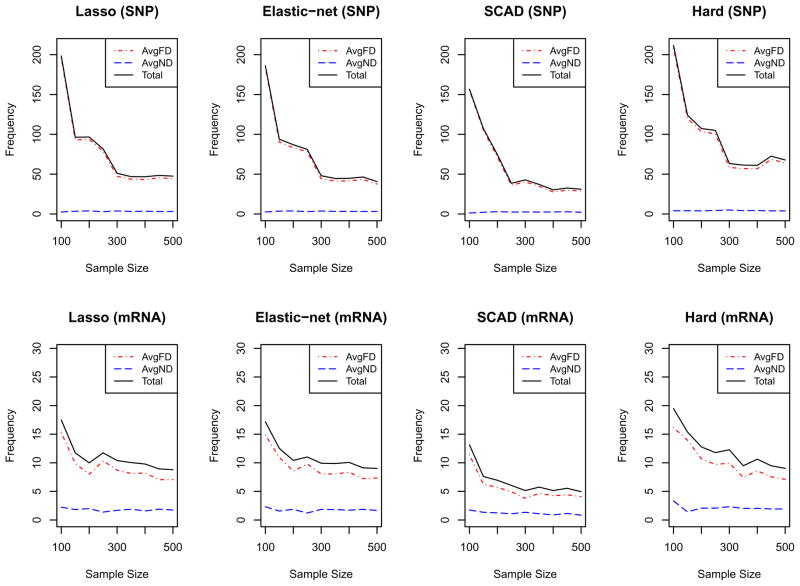
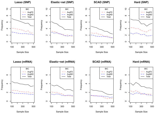
Next, the methods were compared with respect to AvgFD, AvgND and total discordance. Total discordance was computed by adding AvgFD and AvgND. In addition to these, the effects of the sample sizes in the performances of the methods were assessed. Simulations with sample sizes: 100, 150, 200, 250, 300, 350, 400, 450 and 500 were run. For each sample size, 100 simulations were run and AvgFD and AvgND values were computed, with the sum of the AvgFD and AvgND resulting in the total discordance. The AvgFD, AvgND and total discordance values are displayed in Figures 3 (before BIC filter) and 4 (after BIC filter). For SNPs, the AvgND values were consistently low for all sample sizes and penalty functions; however, the AvgFD varied with sample size and penalty function. AvgFD (and hence the total discordance) decreases as sample size increases for all penalties except the Hard-threshold penalty. After a sample size of 300, the penalty functions behave similarly in terms of AvgFD. However, for sample sizes smaller than 300, AvgFD is larger for Lasso and Elastic-net. Similar trends can be seen with the mRNA variables. Thus, there appears to be a strong effect of sample size on the performance (in terms of AvgFD) of the penalty functions. Figure 3 shows that discordances are consistently lowest with SCAD and highest for the Hard-threshold. Figure 3 also shows that the AvgFD decreases with sample size. However, there is still the presence of AvgFD for both SNP and mRNA variables even with a sample size of 500. Application of the BIC filter to SCCA substantially lowered the number of false positive variables as shown in Figure 4. Figure 4 further shows that both AvgND and AvgFD (and hence total discordance) are smaller for the SCAD penalty than other penalty functions.

Figure 3.

For each sub plot, the X-axis represents the sample sizes and the Y-axis represents the values. The top four plots are for SNP variables while the bottom four plots are for mRNA variables. In each plot, the red and blue dotted lines represent the average number of false discovery (AvgFD) and average number of non discovery (AvgND), respectively, and the solid line represents the average total discordance.

Figure 4.

For each sub plot, the X-axis represents the sample sizes and the Y-axis represents the values. Top four plots are for SNPs and the bottom four plots are for mRNA variables. In each plot, the red and blue dotted lines represent the average number of false discovery (AvgFD) and average number of non discovery (AvgND), respectively, and the solid line represents the average total discordance.

In addition, further simulations were carried out under the null association between the SNPs and mRNA expression (with effect size k = 0). None of the variables were selected in more than 5% of simulations before using the BIC filter. After using BIC filter, none of the variables were detected in more than 3% of the simulations.

4 Discussion and Conclusions

It is becoming increasingly common in biomedical research to carry out multiple studies on the same set of subjects. Multiple types of measurements are collected on the same patient sets for such studies and hence integrative analysis approaches are increasingly necessary. Canonical correlation analysis (CCA) is one of the most commonly used data analysis techniques for multiple data sets. However, the traditional CCA has its limitations. It can not be used when the number of variables is larger than the sample size. To overcome this issue, a sparse version of CCA (SCCA) can be implemented. Since SCCA uses only a few important selected variables, it also facilitates the interpretation of the results. SCCA methods proposed in the literature (Waaijenborg et al. 2008; Parkhomenko et al.2009; Le Cao et al.2009; Witten and Tibshirani 2009; Lykou and Whittaker 2009) have either used Lasso or a univariate soft threshold version of the Elastic-net penalty. The goal of this paper is to determine the best penalty function for SCCA involving genomic data in the form of SNPs and mRNA expression.

The SCAD penalty selected the least number of variables while the Elastic-net, Lasso and Hard-thresholding selected more variables (in increasing order). Both the simulation study and the application to the real data showed that SCAD and Elastic-net penalties performed similarity, while the behavior of the hard-threshold penalty was sometimes unpredictable due to the inability to handle multi-collinearity between variables. The additional BIC filter algorithm worked well in removing noise variables, with the relative performance of the four penalty functions preserved after using BIC filter.

Besides choice of a penalty function, the performance of a SCCA method also depends on the approach and criteria for selecting the sparseness parameters. The criteria for selecting sparseness parameters, as outlined by Parkhomenko et al.(2009) and used in the simulation study and real data examples, maximizes the correlation in the test set via cross validation. However, there is a trade off between the maximum correlation and the sparsity of the variables. The more variables are used to compute correlation, the larger the correlation coefficient will be. Therefore, this procedure of determining sparseness parameters alone does not guarantee a sparse solution. Further investigation is needed in determining the sparseness parameters to improve SCCA methods. In addition, this method has only been used for SNP and mRNA expression data. The performance of the method has yet to be assessed with other data types (e.g., phenotypic data, methylation data, microRNA data). This is an area of currently ongoing investigation.

Since the focus of the current paper was to assess the relative performance of the different penalty functions and to demonstrate the need of an additional variable filtering technique in the available SCCA methods, a simple sparse model was used for the simulation studies. However, in many genetic settings, there may be more complex models. For example many SNPs may contribute to the gene expression levels or a few SNPs may be associated with a large number of gene expression levels. The method has yet to be assessed with such complex scenarios. Also, in this manuscript, the matrices X^TX and Y^TY have been replaced with their corresponding diagonal matrices as a regularization technique. We have only looked at this type of regularization as this is the commonly used regularization step in SCCA, such as in Parkhomenko et al. (2009). However, we believe that the results could be generalized to other regularization methods.

The SCCA method can also be applied to large scale genome-wide data sets. However, such an application will be computationally intensive. Therefore, prior dimension reduction steps before using SCCA might be helpful in reducing the computational cost. One of such techniques could be partitioning the SNPs within a gene into bins based on their correlation using a hierarchical clustering method (Rinaldo et al., 2005). Then, principal component analysis (Gauderman et al., 2007) can be carried out for the SNPs within the bin. The first principal component for each bin of SNPs can then be used in the model as the “genetic variable” as opposed to the individual SNP genotypes.

In summary, the previously proposed SCCA methods, which use a Lasso type penalty, yield a large set of selected variables. Therefore, an additional variable filtering method is generally required to achieve effective dimension reduction. In addition, the penalty function used in SCCA can contribute to the performance and sparseness of solution. This research indicates that use of the SCAD penalty for SCCA, with an additional BIC filter, results in the best performance for the analysis of high-dimensional SNP and mRNA expression data sets.

References

- Antoniadis A. Wavelets in Statistics: A review (with discussion) Journal of the Italian Statistical Association. 1997;6:97–144. [Google Scholar]
- Leo Breiman. Better Subset Regression Using the Non-negative Garrote. Technometrics. 1995;37:373–384. [Google Scholar]
- Donoho David L, Johnstone Iain M. Ideal Spatial Adaptation by Wavelet Shrinkage. Biometrika. 1994;81:425–455. [Google Scholar]
- Donoho David L, Johnstone Iain M. Wavelet Shrinkage: Asymptopia? Journal of Royal Statistical Society. 1995;57:301–369. [Google Scholar]
- Jianqing Fan. Commenst on “Wavelets in Statistics: A Review”. Journal of the Italian Statistical Association. 1997;6:131–138. [Google Scholar]
- Jianqing Fan, Runze Li. Variable Selection via Nonconcave Penalized Likelihood and its Oracle Properties. Journal of American Statistical Association. 2001;96:1348–1360. [Google Scholar]
- Gauderman WJ, Murcray C, Gilliand F, Conti DV. Testing association between disease and multiple SNPs in a candidate gene. Genetic Epidemiology. 2007;31:383–395. doi: 10.1002/gepi.20219. [DOI] [PubMed] [Google Scholar]
- Hoerl Arthur E, Kennard Robert W. Ridge regression: Biased estimation for non orthogonal problems. Technometrics. 1970;12:55–57. [Google Scholar]
- Harold Hotelling. Relations between two sets of variants. Biometrika. 1936;28:321–377. [Google Scholar]
- Kim-Anh Le Cao, Martin Pascal GP, Robert Granie Christine, Philippe Besse. Sparse canonical methods for biological data integration: application to a cross-platform study. BMC Bioinformatics. 2009;10 doi: 10.1186/1471-2105-10-34. [DOI] [PMC free article] [PubMed] [Google Scholar]
- Li L, Fridley B, Kalari K, Jenkins G, Batzler A, Safgren S, et al. Gemcitabine and Cytosine Arabinoside Cytotoxicity: Association with Lymphoblastoid Cell Expression. Cancer Res. 2008;68:7050–7058. doi: 10.1158/0008-5472.CAN-08-0405. [DOI] [PMC free article] [PubMed] [Google Scholar]
- Li L, Fridley B, Kalari K, Jenkins G, Batzler A, Weinshilboum RM, et al. Gemcitabine and arabinosylcytosin pharmacogenomics: genome-wide association and drug response biomarkers. PLoS One. 2009;4:e7765. doi: 10.1371/journal.pone.0007765. [DOI] [PMC free article] [PubMed] [Google Scholar]
- Anastasia Lykou, Joe Whittaker. Sparse CCA using a lasso with positivity constraints. Computational Statistics and data Analysis 2009 [Google Scholar]
- Elena Parkhomenko, David Tritchler, Joseph Beyene. Sparse cannical correlation analysis with application to genomic data integration. Statistical Application s in Genetics and Molecular Biology. 2009;8 doi: 10.2202/1544-6115.1406. [DOI] [PubMed] [Google Scholar]
- Rinaldo A, Bacanu SA, Devlin B, Sonpar V, Wasserman L, Roeder K. Characterization of multilocus linkage disequilibrium. Genetic Epidemiology. 2005;28:193–206. doi: 10.1002/gepi.20056. [DOI] [PubMed] [Google Scholar]
- Scheet P, Stephens MA. Fast and Flexible Statistical Model for Large-Scale Population Genotype Data: Applications to Inferring Missing Genotypes and Haplotypic Phase. The American Journal of Human Genetics. 2006;78:629–644. doi: 10.1086/502802. [DOI] [PMC free article] [PubMed] [Google Scholar]
- Robert Tibshirani. Regression shrinkage and selection via the lasso. Journal of Royal Statistical Society B Series. 1996;58:267–288. [Google Scholar]
- Vinod H. Canonical ridge and econometrics of joint production. Journal of Econometrics. 1976;4:117–166. [Google Scholar]
- Waaijenborg Sandra, Philip WittHamer, Zwinderman Aeiko H. Quantifying the Association between gene Expression and DNA-Markesrs by Penalized Canonical Correlation Analysis. Statistical Application s in Genetics and Molecular Biology. 2008;7 doi: 10.2202/1544-6115.1329. [DOI] [PubMed] [Google Scholar]
- Witten Daniela M, Tibshirani Robert J. Extension of sparse canonical correlation analysis with application to genomic data. Statistical Applications in Genetics and Molecular Biology. 2009;8 doi: 10.2202/1544-6115.1470. [DOI] [PMC free article] [PubMed] [Google Scholar]
- Zhijin Wu RAI, Gentleman R, Martinez-Murillo F. A model-based background adjustment for oligonucleotide expression arrays. Forrest Spencer Journal of the American Statistical Association. 2004;99:909. [Google Scholar]
- Jianhui Zhou, Xuming He. Dimension reduction based on constrained canonical correlation and variable filtering. The Annals of Statistics. 2008;36:1649–1668. [Google Scholar]
- Hui Zou, Trevor Hastie. Regularization and variable selection via the elastic net. Journal of Royal Statistical Society. 2005;67:301–320. [Google Scholar]