


Abstract
MEME and many other popular motif finders use the expectation–maximization (EM) algorithm to optimize their parameters. Unfortunately, the running time of EM is linear in the length of the input sequences. This can prohibit its application to data sets of the size commonly generated by high-throughput biological techniques. A suffix tree is a data structure that can efficiently index a set of sequences. We describe an algorithm, Suffix Tree EM for Motif Elicitation (STEME), that approximates EM using suffix trees. To the best of our knowledge, this is the first application of suffix trees to EM. We provide an analysis of the expected running time of the algorithm and demonstrate that STEME runs an order of magnitude more quickly than the implementation of EM used by MEME. We give theoretical bounds for the quality of the approximation and show that, in practice, the approximation has a negligible effect on the outcome. We provide an open source implementation of the algorithm that we hope will be used to speed up existing and future motif search algorithms.
INTRODUCTION
Reverse-engineering transcriptional regulatory networks is a major challenge for today's molecular cell biology. High-throughput methodologies such as ChIP-seq (1), ChIP-chip (2) and DamID (3) are generating ever larger data sets on the binding locations of transcription factors (TFs). However, the resolution of these techniques is still an order of magnitude or two larger than a typical transcription factor binding site (TFBS) (4). There remains a need to determine the binding sequence preferences of TFs and hence the exact locations of TFBSs from these data sets. For example, knowledge of these sequence preferences can be used to computationally predict binding sites in different cell types or in different organisms. In addition, understanding the exact locations of TFBSs for cooperating TFs can help us understand combinatorial transcriptional regulation (5). This task of inferring the sequence preferences of a TF is termed ‘motif finding’.
A typical high-throughput experiment might generate a data set of thousands of sequence fragments. Each fragment could be hundreds of base pairs long. The sequence preferences of a TF are relatively short, typically 8–12 bp. Mismatches to the preferred bases are common in TFBSs. Determining these sequence preferences from the few binding sites in the fragments is a difficult problem. However, much effort has been dedicated to this motif finding problem and many algorithms and softwares exist for this purpose. The area has been reviewed several times (6–9).
Most motif finders can be broadly categorized as either combinatorial or probabilistic. Combinatorial motif finders search for consensus sequences. TFBSs are predicted on the basis of the number of mismatches with these consensus sequences. Probabilistic motif finders infer position weight matrices (PWMs) that specify a distribution of bases for each position in a TFBS. PWMs are more flexible models of TFBSs than consensus sequences and are typically preferred. Most of the probabilistic motif finders use either the expectation–maximization (EM) algorithm (10) or a Gibbs sampling algorithm (11) for inference. Examples of motif finders that use the EM algorithm include Refs (12–20).
The volume of available TF binding location data is rapidly increasing. Both the number and the size of data sets generated by techniques such as ChIP-chip, ChIP-seq and DamID continues to grow. Unfortunately, the runtime of most motif finders is at least linear in the size of the data. In our experience, most motif finders are far too slow for such large data sets of sequences. While it may be possible to let the motif finder run for several days, invariably the user would like to fine-tune parameters. This may involve several runs which makes motif finding impractical.
MEME (13) is one of the most popular motif finders. It has a long pedigree: the original version was published in 1994. MEME was one of the best performing motif finders in a comparative benchmark review (21). MEME has a large user-base that understand its parameters and trust its results: the primary paper describing its algorithm is cited more than 300 times on PubMed. Unfortunately, MEME takes a prohibitively long time to run on large data sets. The MEME authors acknowledge this and recommend discarding data from large data sets in order to make runtimes practical. They suggest a limit of 200 000 bp on the size of input data set. In our experience, the users of MEME are not always aware of this advice and can be frustrated when using MEME on large data sets. In any event, discarding data is a far from ideal work around as it necessarily detracts from the power of the method. Hence there is a need to make MEME and other motif finders more efficient. This article focuses on speeding up the EM algorithm that is a core component of MEME and many other motif finders.
Various attempts have been made to speed up MEME in recognition of its poor performance on large data sets. The authors of MEME have implemented a parallel version of MEME, ParaMEME (22). Other approaches use specialized hardware such as parallel pattern matching chips on PCI cards (23) or off-loading the computations onto powerful GPUs (24). All these techniques require hardware that is not commonly available to the typical researcher.
In this article, we propose an alternative route to accelerate MEME by using suffix trees. A suffix tree (25) is a data structure that represents a sequence or set of sequences. Suffix trees are well suited to algorithms that require efficient access to subsequences by content rather than by position. They have been used in several areas of bioinformatics: sequence alignment (26), indexing genome-scale sequences (27) and short read mapping (28). They have also been used for combinatorial motif finding (29–31) and scanning for PWMs (32). To the best of our knowledge, the work presented here is the first application of suffix trees to probabilistic motif finding and the EM algorithm in particular.
In the ‘Materials and Methods’ section, we describe MEME's probabilistic model and how MEME uses the EM algorithm to optimize its parameters. We describe an approximation to EM and show how suffix trees can be used to implement this approximation (the STEME algorithm). We analyse the expected efficiency gains we expect to achieve with this approximation. We describe our open source implementation of the STEME algorithm. In the ‘Results’ section, we describe the tests we undertook to establish the accuracy and efficiency of STEME in practice. We examine the effect of varying the motif width and the main parameter in our algorithm on the accuracy and efficiency. In the ‘Discussion’ section, we look at the implications of the results and suggest how our algorithm can be best used. We conclude with an outlook for future work.
MATERIALS AND METHODS
MEME
MEME uses the EM algorithm to improve a model of the motif iteratively. In each iteration, the locations of the binding sites are estimated using the current model of the motif and the motif is updated using the predicted sites weighted by their likelihoods. The EM algorithm is guaranteed to converge to a local maximum of the likelihood function but is very sensitive to initial conditions. To mitigate this sensitivity, MEME runs the EM algorithm many times from different starting points.
MEME's model
For a particular motif width, W, MEME treats every subsequence of length W (henceforth W-mer) in the data independently. Given a motif width, W, MEME models each W-mer in the sequences as an independent draw from a two-component mixture. One mixture component models the background sequence composition, the other models binding sites. The binary latent variables, Z = {Z1, … , ZN}, indicate whether each W-mer, Xn, is drawn from the background component or the binding site component. MEME has several different variants of its model which the user can choose between. They vary in how the sites are distributed among the sequences. The oops variant insists that there is exactly One Occurrence Per Sequence. For most experimental data, this is not a realistic assumption and those sequences that do not contain a site can reduce MEME's ability to find the motif. The zoops variant allows Zero or One Occurrences Per Sequence. This is more plausible for most experimental data sets but will not take statistical strength from more than one site in a sequence. The anr variant allows any number of binding sites in each sequence. This variant is the most flexible and is the most suitable for most applications. However, it is also the most computationally demanding: care must be taken in the algorithm when sites overlap otherwise MEME will tend to converge on self-overlapping motifs. This is because MEME's assumption that the W-mers are independent breaks down as each W-mer will overlap with up to 2(W − 1) other W-mers. Nevertheless, as homotypic clusters of binding sites are common in transcriptional networks, we will focus on this anr variant in the rest of this article.
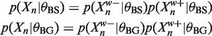
In the anr variant, the background component is modelled using a Markov model parameterized by θBG, the binding site component is modelled by a PWM parameterized by θBS, and λ parameterizes the probability that any given W-mer is drawn from the binding site component. Thus the model is
| (1) |
| (2) |
where {X1, … , XN} are the W-mers and {Z1, … , ZN} are latent variables indicating whether the W-mers are drawn from the background or binding site model. This gives the joint distribution
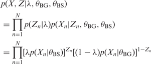 |
(3) |
The model is depicted in plate notation in Figure 1.
Figure 1.
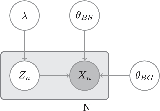
MEME's model: λ, the prior probability of a binding site; Zn, the hidden variable representing whether the n-th W-mer is an instance of the motif; Xn, the n-th W-mer; θBS, the parameters of the motif; θBG, the parameters of the background distribution.
EM
In the E-step of EM, MEME derives the expected value of the log likelihood, LL, w.r.t. the latent variables, Z, given the current parameter estimates, θ = {θBS, θBG, λ}. All expectations, 〈.〉Z|θ, are w.r.t. Z|θ unless specified.
| (4) |
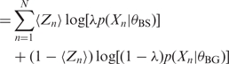 |
(5) |
From Equation (3) and an application of Bayes' theorem
| (6) |
The M-step maximizes the expected log likelihood w.r.t. each parameter in turn to calculate their new estimates. On inspection of (5), we can see
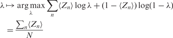 |
(7) |
| (8) |
| (9) |
MEME uses a PWM model for binding sites where θBS = {fwb}. fwb parameterizes the probability of seeing base b at position w in a TFBS.
| (10) |
Here Xnw is the w-th base of the n-th W-mer. The update equations are
| (11) |
where cwb is the expected number of times we see base b at position w in a binding site and S is the expected number of binding sites.
By default, MEME uses a 0-order Markov model for θBG. This is updated by the expected counts of the bases which are not in binding sites.
At the end of each iteration of EM, MEME adjusts its estimates for the Zn. This accounts for the fact that the model does not prohibit overlapping binding sites. By way of explanation, suppose that there are 12 consecutive ‘A’s in the data and the current estimate of the motif models binding sites of eight consecutive ‘A’s. Without this adjustment, MEME would assign 〈Zn〉 ≈ 1 to the 5 W-mers in the consecutive ‘A’s. The sum of the 〈Zn〉 represents the number of binding events we expect in that window. Sterically, five TFs cannot bind to sites of width 8 in a 12 bp window. MEME's algorithm leaves the highest 〈Zn〉 unchanged and scales the others down so that they sum to at most 1. Without this adjustment, repetitive sections in the input sequences can cause MEME to converge on motifs of low complexity that have frequently overlapping binding sites.
Expected running time
Each iteration of MEME's EM algorithm evaluates the current estimate of the motif on each W-mer. The algorithm to adjust for overlaps also runs in O(NW) time hence an iteration of EM completes in O(NW) time. However, it should be noted MEME's algorithm as a whole is quadratic in N as the number of seeds is proportional to N.
Approximation to EM
The updates in the M-step of the EM algorithm all involve sums of the form ∑n 〈Zn〉… where n ranges over all W-mers in the data set. In any given iteration of EM, depending largely on the current θBS, most of these 〈Zn〉 will be negligible. We can make an approximate M-step by ignoring those n for which 〈Zn〉 is small. We formalize this by defining a subset of the n thresholded by 〈Zn〉:
| (12) |
Intuitively, Tδ indexes those W-mers that match our current motif estimate. As an approximation to Equation (11), we define 
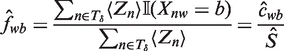 |
(13) |
For convenience of notation, we define 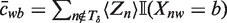 ,
, 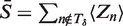 and
and 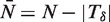 so that
 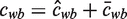 ,
,  and
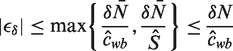
and 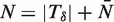 . The relative error, ϵδ, in our approximation
  of fwb is
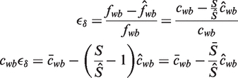 |
Noting that  and all the counts, c, are positive
 |
(14) |
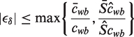
We know from the definition of Tδ that  and that
 |
(15) |
So  . If we knew ĉwb we would know which δ would guarantee our desired bound in the motif estimation relative error. Unfortunately, at the beginning of an EM iteration when we want to choose δ we do not know ĉwb. In practice, this is not a problem. Given λ and the current motif parameters, we can estimate ĉwb fairly accurately. When the EM iteration has completed, ĉwb is available. We can check the above equations to ensure that the relative error is less than |ϵδ|. If it is not, we can calculate a new δ for which the relative error is guaranteed to be small enough and re-run the iteration. In our tests, this was never necessary. Also ĉwb tends to change slowly over iterations, making its estimation straightforward in all but the first iteration.
Suffix trees
A suffix tree is a data structure that stores a sequence or a set of sequences. Typically, sequences are stored as contiguous buffers. This permits fast access to subsequences indexed by their position. Suffix trees are alternative data structures that allow efficient access to subsequences by their content. Re-writing algorithms to use suffix trees can often achieve significant efficiencies.
Suppose we have a sequence, Y = y1… yT. A suffix of Y is any subsequence, yt… yT, that ends at yT. A suffix tree stores every suffix of the given sequence(s) in a tree structure. An example of a suffix tree is shown in Figure 2. Now we show how to iterate over all the subsequences of length W in Y (the W-mers). Each such W-mer is the start of a suffix. Hence, descending the tree to depth W iterates over all the W-mers. If two W-mers have the same content, they will be represented once by the same path in the tree. Contrast this with the random access of a typical contiguous buffer data structure for sequence storage. A contiguous buffer permits fast random access to a W-mer at a given position but takes no account of identical or similar W-mers. If we have an application where we are not interested in the position of the W-mers, a suffix tree can be a more efficient data structure to iterate over them. Another attractive property of suffix trees is that they can be constructed in linear time and space (33).
Figure 2.
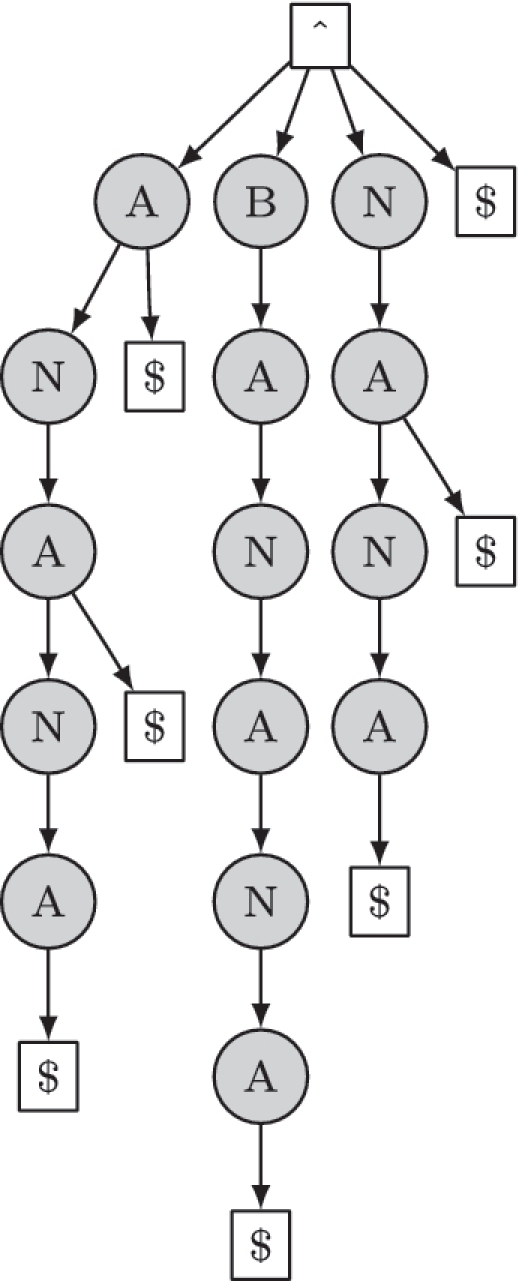
A suffix tree that represents the sequence ‘BANANA’. The beginning of the sequence is represented by the symbol ∧ and $ is a termination symbol. Note that the subsequence ‘ANA’ occurs twice in the sequence but is represented once in the tree.
Suffix tree EM efficiencies
The EM algorithm must visit every W-mer in the sequences once on each iteration. By using a suffix tree to enumerate all the W-mers, we immediately achieve two efficiency improvements. First, if any two W-mers are identical, the 〈Zn〉 calculations are equivalent and we do not repeat them. Second, as we descend the suffix tree to enumerate the W-mers, we make partial evaluations of our current motif on what we have seen of the W-mer so far. These partial evaluations are shared across all the W-mers below the current node in the tree. In contrast, MEME evaluates every base in each W-mer once.
Branch-and-bound
Recall from Equation (12) that we need to identify all n with 〈Zn〉 ≥ δ for a given δ. We iterate over the W-mers by descending the suffix tree. Suppose we have an upper bound on the 〈Zn〉 of all the W-mers below any node. If this bound is below δ, then we can ignore the entire branch of the suffix tree below the node. In this way, we avoid evaluating large parts of the tree that do not fit the current estimate of the motif well. We illustrate the idea in Figure 3.
Figure 3.
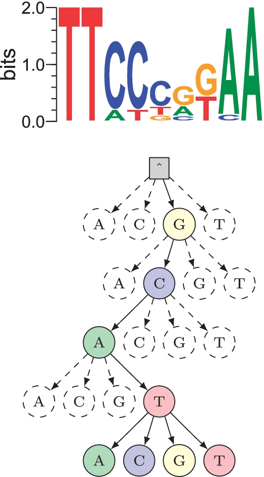
An illustration of how the STEME branch-and-bound algorithm works. Top: the current estimate of the motif in the EM algorithm. This is actually the motif for Stat5 from the TRANSFAC database (M00223). Bottom: part of the suffix tree representing the sequences. We can see that if we have descended the tree to the node that represents the prefix, GCAT, our match to the motif is poor. If the bound for the 〈Zn〉 of all the nodes below this is small enough, we can stop our descent here.
We define  as the prefix of Xn of length w and
  as the suffix of length W − w (so that
 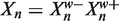 ). We can write the likelihoods of the Xn in terms of their prefixes and suffixes
 |
We can enumerate the W-mers in the data by descending a suffix tree. Each node we visit represents the prefix of all the W-mers below it. Given our binding site and background models, we can calculate the  and
and  exactly. Suppose we can also bound
  from above and
  from below. Recalling (6) we can use these bounds to bound 〈Zn〉 above. In more detail, suppose
 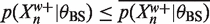 and
and 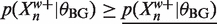 then using 0 as a lower bound for
  we have
 |
(16) |
The upper bounds,  are easy to calculate from θBS. In practice, the background model does not change very much over the course of the EM algorithm as only a small fraction of the base pairs are explained as binding sites. Therefore, we keep the background model fixed and pre-compute the lower bounds,
  , in an initialization step.
Expected efficiencies
In order to understand the computational savings this approximation makes, we give an analysis of a simplified example. We investigate the expected fraction of nodes we ignore at each depth in our descent of the suffix tree.
Suppose our current estimate of the PWM has a preferred base at each position. Each preferred base has probability a and the other three bases at each position are equally likely with probability  . When a = 1, our PWM is equivalent to a consensus sequence, when
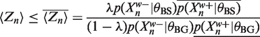
  our PWM has a uniform distribution. As ĉwb ≈ λNa we set δ = ϵλa where ϵ is the maximum relative error we will tolerate. Suppose also our background model is a uniform 0-order Markov model, then p(Xn|θBG) = 4−W. As 1 ≈ 1 − λ and recalling (16), we want to know when the following holds
Let Y be the number of preferred bases in  . Assuming that
  is drawn from our background distribution, we have Y ~ Binomial(w,
  ). Now
  . Hence whenever
| (17) |
we can ignore all the nodes with prefix  . For any given values of ϵ, W and a, the expected fraction of nodes ignored at depth w is the probability that Equation (17) holds. As Y is distributed according to a binomial distribution, these values can be read directly from the binomial cumulative distribution function. We plot these expected fractions for some parameter values in Figure 4.
Figure 4.

The probability of discarding a W-mer drawn from a uniform 0-order Markov background at different depths, w, in the suffix tree. Here we used ϵ = 0.4. As explained in the text, a represents how sharp the current estimate of the motif is. The higher a is, the sharper the motif. Examining the graph reveals that with a moderately sharp motif (a = 0.7) of width 8, we can expect to discard over half the nodes in the tree at depth w = 6.
Open source implementation
We have implemented the STEME algorithm in C++ as an open source library. For the suffix tree implementation, we used the SeqAn library (34). In addition to the C++ interface we have implemented a Python scripting interface to make it more accessible. The codes are tested on Linux with GCC 4.4 and Python 2.6 but should work with any modern C++ compiler and version of Python 2 newer than 2.5. Our implementation is available at http://sysbio.mrc-bsu.cam.ac.uk/johns/STEME/. Our implementation requires 500 Mb of memory to work with data sets of up to 13 Mb, which is well within the range of modern desktop or laptop machines. Building the suffix tree for such a data set takes 19 s on our laptop. These space and time requirements scale linearly in the size of the input.
Test data sets
We used data from two sources for our tests (Table 1): a set of six smaller ChIP-chip and ChIP-seq data sets we had previously worked with (35); and five larger data sets from the ENCODE project (36).
Table 1.
The test data sets
The six data sets we had previously worked with were prepared as follows. The data for Sp1 were extracted from TRANSFAC Professional 11.4 and the flanking bases added by TRANSFAC were removed. The data sets for GABP, Stat1, Stat5a and Stat5b were processed to extract the binding site sequences using the cisGenome software suite v1.0 (41). In every case, both sequences and controls were used. Binding region boundary refinement was used and then the region extended on each side by 30 bp. GABP peaks were selected if there were more than 18 reads in a rolling 100 bp sequence window compared with the control. This higher figure was selected to remove visually noisy peaks and 10 767 peaks were detected. Cut-offs of 30 and 20 reads were used for the Stat5a and Stat5b data, respectively, yielding 814 and 154 peaks. RepeatMasker was used on all the test data sets to mask repetitive elements using the genomic context for each sequence. We provide the sequences as part of the Supplementary Data. These files give data for sequences and genomic coordinates. The results in the article are based on the masked data, but the unmasked data are given for completeness. The sequences are given in FASTA format and notes about the files for genomic coordinates (including assembly versions) are given within the files.
The five larger data sets from the ENCODE project were produced by the Myers Lab at the HudsonAlpha Institute for Biotechnology. We downloaded the data for SRF, ZBTB33, RXRA, TCF12 and CTCF from the ENCODE Data Coordination Center at UCSC.
Tests
In order to test the accuracy and efficiency of the STEME approximation, we ran our STEME implementation and MEME's EM implementation to completion on the data sets.
We wanted to try a range of typical parameters so we ran MEME's seed searching algorithm with the default arguments. We used motif widths of 8, 11, 15 and 20. The number of site parameters took values of 2, 4, 8, 16, 32, 64, 128, 256 and 500. MEME uses the number of sites parameter to initialize λ and also to look for the best seed (consensus sequence) for the motif. This gave us 6 data sets, 4 motif widths and 6 different number of sites parameters for a total of 144 separate test cases. Additionally, we wanted to test the effect of varying the permitted relative error so when we ran STEME, we used ϵs of 0, 0.2, 0.4, 0.6 and 0.8.
Once we had run the test cases, we needed some way of comparing the results of the different implementations and the different settings for the permitted relative error, ϵ. Comparison of the resulting PWMs would have been possible but we chose to perform a simplified analysis by converting the resulting PWMs into consensus sequences and using the Hamming distance as a distance metric. To test the accuracy of the STEME approximation, we calculated two statistics: the mismatch rate, that is, how often the resulting consensus sequences from the same starting point differed in any base; and the mismatch fraction, that is, what proportion of the bases of the resulting consensus sequences differed.
We ran the tests using version 4.5.0 of MEME which was released on 8 October 2010. We modified the MEME source code in order to obtain precise timing information for its EM algorithm. The modifications are available as a patch included with the STEME source code.
RESULTS
How ϵ affects STEME's accuracy
We compared the accuracy of STEME when using different bounds on the relative error, ϵ. When ϵ = 0, no approximations are made and we used this as a baseline for comparison. The average mismatch rate and mismatch fraction statistics are plotted in Figure 5. Even when a very large relative error of 0.8 is permitted, only 1 in 6 of the resulting consensus sequences differ and less than 1 in 20 bases differ. When using a reasonable value of ϵ = 0.4, only around 1 in 8 of the test cases differed from the baseline and only 1 in 30 of the resulting bases differed.
Figure 5.

An analysis of how increasing the permitted relative error, ϵ, affects the outcome of STEME. The STEME algorithm was run from the initializations described in the text for various values of ϵ. (A) The mismatch rate: The fraction of resulting consensus sequences that differed from those when ϵ = 0. (B) The mismatch fraction: The fraction of bases in the resulting consensus sequences that differed from those when ϵ = 0.
STEME's accuracy relative to MEME
We also analysed the accuracy of STEME relative to MEME. We had hoped that the STEME algorithm with the approximation turned off (ϵ = 0) would produce identical results to MEME. For reasons we present in the ‘Discussion’ section, this is not the case. These results are presented in Figure 6. When ϵ = 0, less than 1 in 4 of the test cases had a different outcome but only about 1 in 20 of the bases in the resulting consensus sequences differed. As an example, when the seed ‘ATCCTGTTCTC’ is used with 16 sites on the Sp1 data set, MEME converges to ‘CTTCCTTCTCT’ and STEME converges to ‘CTCCCTTCTCT’.
Figure 6.

An analysis of the accuracy of STEME for various values of ϵ relative to MEME. The STEME algorithm was run from from the initializations described in the text for various values of ϵ. (A) The mismatch rate: the fraction of resulting consensus sequences that differed from the results of MEME. (B) The mismatch fraction: the fraction of bases in the resulting consensus sequences that differed from the results of MEME.
Efficiency
We compared the runtime for an iteration of STEME to an iteration of the MEME EM algorithm. The relative speeds are dependent on the value of ϵ chosen and on the width of the motif, as shown in Figure 7. STEME is significantly quicker than MEME for reasonable values of ϵ and typical motif widths.
Figure 7.

A comparison of the speed of STEME and MEME on one iteration of the EM algorithm. (A) Using ϵ = 0.4 as a typical setting, the iteration speeds across all the data sets are plotted on a log 10 scale. The error bars represent the standard deviations. (B) A violin plot of the relative speeds of MEME and STEME grouped by ϵ. With ϵ = 0, STEME can be slower than MEME although we would expect this to reverse on larger data sets. As ϵ grows, STEME's advantage grows. The contours of the violin plots are kernel density estimates that are truncated at the minimum and maximum values. The y-axes are on a log 10 scale. (C) Using ϵ = 0.4 as a typical setting, the relative speeds grouped by motif width. For motifs of width 8, STEME is between 10.3 ≃ 2 and 102.1 ≃ 125 times quicker than MEME.
DISCUSSION
Accuracy
Examining Figure 5 we can see that when ϵ = 0.4 about 1 in 8 of our applications of EM had some discrepancy with the exact algorithm and about 1 base in 30 differed overall. In our experience, this represents a satisfactory compromise of speed and accuracy. In any case, it is not clear if all the differences introduced by the approximation have a negative effect. Our approximation ignores those putative binding sites that are not a good match to the motif rather than discounting them. It could be that by only examining the higher quality binding sites, our algorithm builds a better model of the motif. We hope to investigate this possibility in further work integrating our STEME algorithm in a motif finder.
We also compared STEME without any approximation to MEME's EM implementation (Figure 6). We had hoped the implementations would agree. Unfortunately, there were some discrepancies. We spent some time reverse engineering the MEME source code and discovered some inconsistencies between the published MEME algorithm (42) and the latest implementation. In particular, the handling of reverse complements is not discussed in the published algorithm. STEME treats each draw as a 50/50 mixture between a binding site on the positive strand and a binding site on the negative strand. The MEME implementation essentially doubles the size of the data by adding a reverse-complemented copy of the data. Despite this, STEME and MEME converge on essentially the same motifs. On average, only 1 base in 20 differs.
Interestingly, it appears that there is significant overlap between the test cases for which STEME without any approximation differs from MEME and those test cases for which the result of the STEME changes as the permitted error is allowed to grow. This can be seen in Figure 6 as the difference between ϵ = 0 and ϵ = 0.4 is smaller than the analogous difference in Figure 5.
Efficiency
Figure 7 shows that the speed-up possible through the STEME approximation is dependent both on the width of the motif considered and the relative error tolerated in the estimation of the motif. For motifs of reasonable size (W = 8 or 11), an order of magnitude increase in speed over MEME can be expected when using a relative error of ϵ = 0.4. Our approximation is consistently quicker than MEME's implementation of EM which is already highly optimized. STEME achieves an order of magnitude increase in speed on data sets of moderate size for a wide range of reasonable parameters. In the coming years, we expect the average size of data sets to continue increasing.
Applicability
We have not presented a complete motif finder but we have shown how any motif finder that uses the EM algorithm on a compatible model can be adapted to handle larger data sets. We would have liked to have presented an efficient drop-in replacement for MEME but were prevented from doing so for some technical reasons that we elaborate on here.
The EM algorithm is not a motif finder on its own. The result of EM is dependent on how the parameters are seeded. Hence to find motifs, suitable seeds must be found. MEME's search for seeds is inefficient on large data sets. Integrating our fast EM algorithm with MEME's slow search for seeds would offer little benefit as runtimes would be dominated by the seed search. We are working on using suffix trees to re-implement MEME's search for seeds more efficiently; however, this is a major undertaking in its own right. We have included an implementation of our work-in-progress with the source code for STEME. It is of practical value for motifs of up to width 8 on large data sets (over 500 Kb); however, the efficiencies tail off quickly as the motif width increases (Table 2). For example, on the 674 Kb SRF data set, MEME took over 4 h to find a motif of width 8. In contrast, our implementation with STEME finished in 13 min, 18 times quicker.
Table 2.
Timings for STEME with search for seeds and complete MEME algorithm
| TF | Base pairs (kb) | W | STEME (s) | MEME (s) | Speed-up |
|---|---|---|---|---|---|
| SRF | 674 | 8 | 792 | 14 760 | 18 |
| ZBTB33 | 1 590 | 8 | 933 | 78 339 | 84 |
| TCF12 | 12 540 | 8 | 2122 | 4 928 532 | 2322 |
| TCF12 | 12 540 | 10 | 27 424 | 5 176 744 | 189 |
| TCF12 | 12 540 | 12 | 379 891 | 4 597 053 | 12 |
The times to run MEME on the TCF12 data set are estimated from partial runs as otherwise they would have taken months to complete.
In addition, the way that MEME calculates the significance of the motifs involves a preprocessing step that does not scale well to large numbers of sites. Typically, a user will want to choose the number of sites proportionally to the number of sequences in the data set. Hence for large data sets, the significance calculation needs to be re-implemented more efficiently. We are working on this using approximations to the LLR P-value calculations.
CONCLUSION
Reverse engineering transcriptional networks remains an important in silico challenge. Modern biology continues to generate ever larger data sets and this trend can be expected to continue. Hence there exists a need for good motif finders that can handle large data sets. MEME is well trusted but does not handle these data sets well. We have presented an approximation to EM for models of the type used in the MEME algorithm. We have demonstrated that this approximation has a minor effect on the outcome on the algorithm and is an order of magnitude faster. We have supplied an implementation of this algorithm and hope that it will be incorporated into existing and novel motif finders.
SUPPLEMENTARY DATA
Supplementary Data are available at NAR Online.
FUNDING
Funding for open access charge: Medical Research Council.
Conflict of interest statement. None declared.
Supplementary Material
REFERENCES
- 1.Park PJ. ChIP-seq: advantages and challenges of a maturing technology. Nat. Rev. Genet. 2009;10:669–680. doi: 10.1038/nrg2641. [DOI] [PMC free article] [PubMed] [Google Scholar]
- 2.Liu XS, Meyer CA. ChIP-Chip: algorithms for calling binding sites. Methods Mol. Biol. 2009;556:165–175. doi: 10.1007/978-1-60327-192-9_12. [DOI] [PMC free article] [PubMed] [Google Scholar]
- 3.Southall TD, Brand AH. Chromatin profiling in model organisms. Brief. Funct. Genomic Proteomic. 2007;6:133–140. doi: 10.1093/bfgp/elm013. [DOI] [PubMed] [Google Scholar]
- 4.Gilchrist DA, Fargo DC, Adelman K. Using ChIP-chip and ChIP-seq to study the regulation of gene expression: genome-wide localization studies reveal widespread regulation of transcription elongation. Methods. 2009;48:398–408. doi: 10.1016/j.ymeth.2009.02.024. [DOI] [PMC free article] [PubMed] [Google Scholar]
- 5.Reid JE, Ott S, Wernisch L. Transcriptional programs: modelling higher order structure in transcriptional control. BMC Bioinformatics. 2009;10:218. doi: 10.1186/1471-2105-10-218. [DOI] [PMC free article] [PubMed] [Google Scholar]
- 6.Hu J, Li B, Kihara D. Limitations and potentials of current motif discovery algorithms. Nucleic Acids Res. 2005;33:4899–4913. doi: 10.1093/nar/gki791. [DOI] [PMC free article] [PubMed] [Google Scholar]
- 7.MacIsaac KD, Fraenkel E. Practical strategies for discovering regulatory DNA sequence motifs. PLoS Comput. Biol. 2006;2:e36. doi: 10.1371/journal.pcbi.0020036. [DOI] [PMC free article] [PubMed] [Google Scholar]
- 8.D'haeseleer P. How does DNA sequence motif discovery work? Nat. Biotechnol. 2006;24:959–961. doi: 10.1038/nbt0806-959. [DOI] [PubMed] [Google Scholar]
- 9.Das MK, Dai H-K. A survey of DNA motif finding algorithms. BMC Bioinformatics. 2007;8(Suppl. 7):S21. doi: 10.1186/1471-2105-8-S7-S21. [DOI] [PMC free article] [PubMed] [Google Scholar]
- 10.Dempster AP, Laird NM, Rubin DB. Maximum likelihood from incomplete data via the EM Algorithm. J. Roy. Stat. Soc. Ser. B. 1977;39:1–38. [Google Scholar]
- 11.Geman S, Geman D. Stochastic relaxation, Gibbs distributions and the Bayesian restoration of images. J. Appl. Stat. 1993;20:25–62. doi: 10.1109/tpami.1984.4767596. [DOI] [PubMed] [Google Scholar]
- 12.Lawrence CE, Reilly AA. An expectation maximization (EM) algorithm for the identification and characterization of common sites in unaligned biopolymer sequences. Proteins. 1990;7:41–51. doi: 10.1002/prot.340070105. [DOI] [PubMed] [Google Scholar]
- 13.Bailey TL, Elkan C. 1994. Fitting a mixture model by expectation maximization to discover motifs in biopolymers. Proc. Int. Conf. Intell. Syst. Mol. Biol., 2, 28–36. [PubMed] [Google Scholar]
- 14.Blekas K, Fotiadis DI, Likas A. Greedy mixture learning for multiple motif discovery in biological sequences. Bioinformatics. 2003;19:607–617. doi: 10.1093/bioinformatics/btg037. [DOI] [PubMed] [Google Scholar]
- 15.Prakash A, Blanchette M, Sinha S, Tompa M. Motif discovery in heterogeneous sequence data. Pac. Symp. Biocomput. 2004;1:348–359. doi: 10.1142/9789812704856_0033. [DOI] [PubMed] [Google Scholar]
- 16.Sinha S, Blanchette M, Tompa M. PhyME: a probabilistic algorithm for finding motifs in sets of orthologous sequences. BMC Bioinformatics. 2004;5:170. doi: 10.1186/1471-2105-5-170. [DOI] [PMC free article] [PubMed] [Google Scholar]
- 17.Moses AM, Chiang DY, Eisen MB. Phylogenetic Motif Detection by Expectation Maximization on Evolutionary Mixtures. Pac. Symp. Biocomput. 2004:324–335. doi: 10.1142/9789812704856_0031. [DOI] [PubMed] [Google Scholar]
- 18.Qi Y, Ye P, Bader JS. Genetic interaction motif finding by expectation maximization--a novel statistical model for inferring gene modules from synthetic lethality. BMC Bioinformatics. 2005;6:288. doi: 10.1186/1471-2105-6-288. [DOI] [PMC free article] [PubMed] [Google Scholar]
- 19.MacIsaac KD, Gordon DB, Nekludova L, Odom DT, Schreiber J, Gifford DK, Young RA, Fraenkel E. A hypothesis-based approach for identifying the binding specificity of regulatory proteins from chromatin immunoprecipitation data. Bioinformatics. 2006;22:423–429. doi: 10.1093/bioinformatics/bti815. [DOI] [PubMed] [Google Scholar]
- 20.Li L. GADEM: a genetic algorithm guided formation of spaced dyads coupled with an EM algorithm for motif discovery. J. Comput. Biol. 2009;16:317–329. doi: 10.1089/cmb.2008.16TT. [DOI] [PMC free article] [PubMed] [Google Scholar]
- 21.Tompa M, Li N, Bailey TL, Church GM, Moor BD, Eskin E, Favorov AV, Frith MC, Fu Y, Kent WJ, et al. Assessing computational tools for the discovery of transcription factor binding sites. Nat. Biotechnol. 2005;23:137–144. doi: 10.1038/nbt1053. [DOI] [PubMed] [Google Scholar]
- 22.Grundy WN, Bailey TL, Elkan CP. ParaMEME: a parallel implementation and a web interface for a DNA and protein motif discovery tool. Comput. Appl. Biosci. 1996;12:303–310. doi: 10.1093/bioinformatics/12.4.303. [DOI] [PubMed] [Google Scholar]
- 23.Sandve GK, Nedland M, Syrstad ØB, Eidsheim LA, Abul O, Drabløs F. Workshop on Algorithms in Bioinformatics (WABI)'06. 2006. pp. 197–206. [Google Scholar]
- 24. Chen, C., Schmidt, B., Weiguo, L., and Müller-Wittig, W. (2008) GPU-MEME: Using Graphics Hardware to Accelerate Motif Finding in DNA Sequences. In Chetty, M., Ngom, A., and Ahmad, S., (eds), Pattern Recognition in Bioinformatics, Lecture Notes in Computer Science. Springer, Berlin/Heidelberg, pp. 448–459.
- 25.Gusfield D. Algorithms on Strings, Trees, and Sequences: Computer Science and Computational Biology. Cambridge UK: Cambridge University Press; 1997. [Google Scholar]
- 26.Schatz M, Trapnell C, Delcher A, Varshney A. High-throughput sequence alignment using Graphics Processing Units. BMC Bioinformatics. 2007;8:474. doi: 10.1186/1471-2105-8-474. [DOI] [PMC free article] [PubMed] [Google Scholar]
- 27.Phoophakdee B, Zaki MJ. In 13th Pacific Symposium on Biocomputing. World Scientific Publishing Company: 2008. pp. 90–101. [PubMed] [Google Scholar]
- 28. Mäkinen, V., Välimäki, N., Laaksonen, A., and Katainen, R. (2010) Unified view of backward backtracking in short read mapping. In Elomaa, T., Mannila, H., and Orponen, P. (eds), Algorithms and Applications, Lecture Notes in Computer Science. Springer, Berlin/ Heidelberg, pp. 182–195.
- 29.Federico M, Pisanti N. Suffix tree characterization of maximal motifs in biological sequences. Theor. Comput. Sci. 2009;410:4391–4401. [Google Scholar]
- 30.Marsan L, Sagot MF. Algorithms for extracting structured motifs using a suffix tree with an application to promoter and regulatory site consensus identification. J. Comput. Biol. 2000;7:345–362. doi: 10.1089/106652700750050826. [DOI] [PubMed] [Google Scholar]
- 31.Pavesi G, Mauri G, Pesole G. An algorithm for finding signals of unknown length in DNA sequences. Bioinformatics. 2001;17(Suppl. 1):S207–S214. doi: 10.1093/bioinformatics/17.suppl_1.s207. [DOI] [PubMed] [Google Scholar]
- 32.Beckstette M, Homann R, Giegerich R, Kurtz S. Fast index based algorithms and software for matching position specific scoring matrices. BMC Bioinformatics. 2006;7:389. doi: 10.1186/1471-2105-7-389. [DOI] [PMC free article] [PubMed] [Google Scholar]
- 33.Ukkonen E. On-line construction of suffix trees. Algorithmica. 1995;14:249–260. [Google Scholar]
- 34.Döring A, Weese D, Rausch T, Reinert K. SeqAn an efficient, generic C++ library for sequence analysis. BMC Bioinformatics. 2008;9:11. doi: 10.1186/1471-2105-9-11. [DOI] [PMC free article] [PubMed] [Google Scholar]
- 35.Reid JE, Evans KJ, Dyer N, Wernisch L, Ott S. Variable structure motifs for transcription factor binding sites. BMC Genomics. 2010;11:30. doi: 10.1186/1471-2164-11-30. [DOI] [PMC free article] [PubMed] [Google Scholar]
- 36.Birney E, Stamatoyannopoulos JA, Dutta A, Guigó R, Gingeras TR, Margulies EH, Weng Z, Snyder M, Dermitzakis ET, Thurman RE, et al. Identification and analysis of functional elements in 1 the encode pilot project. Nature. 2007;447:799–816. doi: 10.1038/nature05874. [DOI] [PMC free article] [PubMed] [Google Scholar]
- 37.Liao W, Schones DE, Oh J, Cui Y, Cui K, Roh T-Y, Zhao K, Leonard WJ. Priming for T helper type 2 differentiation by interleukin 2-mediated induction of interleukin 4 receptor alpha-chain expression. Nat. Immunol. 2008;9:1288–1296. doi: 10.1038/ni.1656. [DOI] [PMC free article] [PubMed] [Google Scholar]
- 38.Cawley S, Bekiranov S, Ng HH, Kapranov P, Sekinger EA, Kampa D, Piccolboni A, Sementchenko V, Cheng J, Williams AJ, et al. Unbiased mapping of transcription factor binding sites along human chromosomes 21 and 22 points to widespread regulation of noncoding RNAs. Cell. 2004;116:499–509. doi: 10.1016/s0092-8674(04)00127-8. [DOI] [PubMed] [Google Scholar]
- 39.Valouev A, Johnson DS, Sundquist A, Medina C, Anton E, Batzoglou S, Myers RM, Sidow A. Genome-wide analysis of transcription factor binding sites based on ChIP-Seq data. Nat. Methods. 2008;5:829–834. doi: 10.1038/nmeth.1246. [DOI] [PMC free article] [PubMed] [Google Scholar]
- 40.Robertson G, Hirst M, Bainbridge M, Bilenky M, Zhao Y, Zeng T, Euskirchen G, Bernier B, Varhol R, Delaney A, et al. Genome-wide profiles of STAT1 DNA association using chromatin immunoprecipitation and massively parallel sequencing. Nat. Methods. 2007;4:651–657. doi: 10.1038/nmeth1068. [DOI] [PubMed] [Google Scholar]
- 41.Ji H, Jiang H, Ma W, Johnson DS, Myers RM, Wong WH. An integrated software system for analyzing ChIP-chip and ChIP-seq data. Nat. Biotechnol. 2008;26:1293–1300. doi: 10.1038/nbt.1505. Nov. [DOI] [PMC free article] [PubMed] [Google Scholar]
- 42.Bailey TL, Elkan C. Unsupervised Learning of Multiple Motifs In Biopolymers Using EM. Mach. Learn. 1995:51–80. [Google Scholar]
Associated Data
This section collects any data citations, data availability statements, or supplementary materials included in this article.