Optimization of Nonlinear Dose- and Concentration-Response Models Utilizing Evolutionary Computation

Abstract

An essential part of toxicity and chemical screening is assessing the concentrated related effects of a test article. Most often this concentration-response is a nonlinear, necessitating sophisticated regression methodologies. The parameters derived from curve fitting are essential in determining a test article’s potency (EC₅₀) and efficacy (E_max) and variations in model fit may lead to different conclusions about an article’s performance and safety. Previous approaches have leveraged advanced statistical and mathematical techniques to implement nonlinear least squares (NLS) for obtaining the parameters defining such a curve. These approaches, while mathematically rigorous, suffer from initial value sensitivity, computational intensity, and rely on complex and intricate computational and numerical techniques. However if there is a known mathematical model that can reliably predict the data, then nonlinear regression may be equally viewed as parameter optimization. In this context, one may utilize proven techniques from machine learning, such as evolutionary algorithms, which are robust, powerful, and require far less computational framework to optimize the defining parameters. In the current study we present a new method that uses such techniques, Evolutionary Algorithm Dose Response Modeling (EADRM), and demonstrate its effectiveness compared to more conventional methods on both real and simulated data.

1. INTRODUCTION

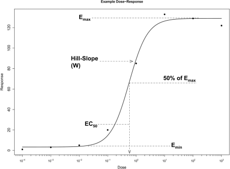
Nonlinearity is a pervasive phenomenon in biological systems (Schnell et. al 2007). Processes such as mRNA expression (Vanden Heuvel, et al. 1994, Hariparsad et. al 2008), neural networks (Rolls and Treves 1998), and metabolic networks all have an input/output relationship that is nonlinear. Moreover, such systems often exhibit sigmoidal or exponential responses in the presence of increasing stimuli. However, it is typically not feasible to have inputs that are truly continuous; instead an investigator must partition the input space into discrete pieces comprising a representative range. Thus, a crucial task for any researcher is the process of information recovery, as an experiment cannot be run with infinite precision the researcher must interpolate the missing information between these discrete observations. An example of a prototypical sigmoid response is given in Figure 1.

FIGURE 1:

Example Nonlinear Dose-Response

One traditionally used approach in dose-response modeling has been to use an implementation of nonlinear least squares (NLS) (Pinheiro et al. 2006). Some well-known algorithms that implement NLS are the NL2SOL algorithm (Dennis et al. 1981) from the Port package (http://netlib.bell-labs.com/netlib/port/) and the Gauss-Newton method (Bates and Watts 1988). These techniques are taken from the wealth of research in nonlinear regression analysis and attempt to minimize the least squares estimator (Bates and Watts 1988; Dennis et al. 1981). Section 1.3 will discuss these two algorithms in further detail.

While there is a rich history of using NLS for dose response modeling, there are several disadvantages to the method that are of concern. First, model fitting with NLS methods are highly sensitive to the initial parameter values used, resulting in inconsistent parameter estimates or lack of model convergence (Bates and Watts 1988). Additionally, the local search optimization used in NLS modeling can limit the potential of parameter estimation in the presence of complex fitness landscapes, preventing the algorithms from discovering the globally optimal solution (Bates and Watts 1988).

To address these concerns, we propose the use of an Evolutionary Algorithm (EA) to perform the search and optimization for the dose-response model. EAs are search methods inspired by the biological concepts of “natural selection” and “survival of the fittest”. EAs differ from more traditional optimization techniques in that they involve a search from a “population” of solutions, not just a single point. EAs iterate using a competitive selection that weed out poor solutions, and the solutions with high “fitness” (the best fitting solutions) are recombined and mutated in each iteration to “evolve” the best possible solution. EAs have a rich history in optimizing nonlinear models in diverse areas such as engineering (Oyama and Liou 2001), genetics (Motsinger-Reif et al. 2008; Motsinger-Reif and Ritchie 2008), and even air traffic control (Delahaye and Puechmorel 2004). Additionally, other machine-learning approaches have been successfully applied to dose-response data (Chamjangali et al. 2007), indicating the potential of such a strategy. Given the success of EAs in such disparate areas and the comparatively modest mathematical requirements, we believe that our approach is a viable alternative to traditional ones for those wishing to do high-throughput dose-response modeling. In the current manuscript we describe the use of an EA for dose response modeling (EADRM) and its implementation. Additionally, we show the results of an extensive configuration parameter sweep to evaluate the stability of the EADRM solutions and determine optimal configuration parameters. Then we demonstrate its empirical success in detecting a range of simulated dose response models and a real response dataset. Additionally, we compare the performance of the EADRM algorithm to two commonly used NLS algorithms, and demonstrate the improved relative performance of the EADRM method in regards to both model fit and computational requirements.

The rest of this paper is divided as follows: Section 1 provides a general introduction to evolutionary algorithms and an overview of traditional NLS approaches. Section 2 describes the EADRM and NLS implementations, the mathematical models used, and the testing methodology and environment. Section 3 describes the simulation experiments evaluating a range of different parameter settings for the EADRM algorithm, as well as the empirical comparisons of the new method with the traditional NLS approaches. Finally, Section 4 will discuss the results and possibilities for future directions.

1.1. Overview of Evolutionary Algorithms (EAs)

As previously mentioned, EAs are a set of general machine-learning approaches inspired by Darwinian evolution and the concept of survival of the fittest (Fogel et al 1966; Holland 1975) to automatically “evolve” optimal models for the data at hand. EAs maintain a pool of potential models/solutions (population) comprised of initial estimates of the solution (individuals). Each individual has some measure of relative quality, often a measure of model fit (fitness) that is specified by the user. High quality solutions (those models with the highest fitness) are selected for “reproduction” during the iterations (generations) of the EA process. These selected models/solutions then undergo one or more evolutionary operators (i.e. crossover, mutation, duplication, etc.). These operators are used to generate new models/solutions that are biased towards regions of the search space for which good solutions have previously been observed. This iterative process results in the development of increasingly “fit” models/solutions (Koza 1995). This iterative process continues until the solution converges (where fitness becomes maximal and/or unchanging across a number of generations), or until a pre-specified number of generations are completed. There are many specific algorithms that all use this general EA approach, including genetic algorithms, and genetic programming (Koza 1995). For the current study, we use a very general EA approach as described in detail below.

1.2. Nonlinear Regression and Nonlinear Least Squares

Nonlinearity occurs if the observational data can be modeled by a nonlinear combination of the input parameters and has one or more independent variables. A generalized nonlinear model, using the notation from (Bates and Watts 1988), may be written as Equation 1.1:

$$Y_n=f(x_n,\Theta )+Z_n$$

where, in this context, Y_n is the nth observation, f is the expectation function (i.e. the “prediction” function), and x_n is a vector of regressor or independent variables for the nth case. The expectation function is entirely deterministic whereas Z_n represents the nondeterministic or stochastic portion (Bates and Watts 1998) of the response and is often referred to as the noise or disturbance. For a function to be nonlinear at least one of the derivatives of the function with respect to its parameters is dependent upon on at least one of the parameters. This is the crucial difference between linear and nonlinear models.

One of the most elementary examples of this requirement is the exponential decay function which may be expressed as Equation 1.2:

$$f(t,\Theta )=e^{-\Theta t}$$

and whose derivative with respect to Θ is Equation 1.3:

$$\partial f/\partial \Theta =-t{e}^{-\Theta t}$$

Since the derivate of f is dependent upon Θ, the function is nonlinear.

Nonlinear least squares attempts to model nonlinear data by making linear approximations of the model and then iteratively improving these approximations based on the least squares estimator. The least squares estimator is a measure of the sum of squares expressed as Equation 1.4:

$$\sum _{i=1}^n{(y_i-f(x_i,\Theta ))}^2$$

In the context of regression analysis, this definition of sum of squares is a measure of the residuals, or error, associated with a given prediction function. Note that unlike the more familiar linear least squares, nonlinear least squares solutions are not guaranteed to be unique.

1.2.1. Gauss-Newton Method

The Gauss-Newton algorithm is a special case of Newton’s method for finding the minimum of a function and can only be used on sum of squares minimization problems. The approach takes an initial guess of the parameters (Θ⁰) and continues to improve upon this estimate until the solution converges; meaning that the improvement obtained from further iterations is so small that there is no “useful” change to the parameter estimates. More specifically, the method solves the least squares problem for a linear approximation of the function in the region “near” the initial guess, Θ⁰, then replaces the initial value with the linear least squares solution, and iterates until convergence. To minimize the approximate residual sum of squares, the Gauss increment (δ) is computed using a Jacobian matrix of the residuals with respect to Θ, which requires computing a matrix of first-order partial derivatives. For a more in depth explanation refer to (Björck 1996; Bates and Watts 1998).

1.2.2. NL2SOL

NL2SOL is a gradient based, hill-climbing approach to nonlinear least squares. This approach maintains a secant approximation to the second order portion of the least-squares Hessian matrix and then dynamically determines when this approximation is appropriate. The approximation is then scaled, updated, and the process iterates while attempting to minimize a local quadratic model of the sum of squares function constrained to an elliptical trust region centered at the current approximate minimizer. This process requires computing the Hessian matrix, which is comprised of second order partial derivatives and requires numerical approximations that are cumbersome and computationally expensive. Less formally stated this approach uses a gradient to guide the algorithm iteratively to a least squares estimate. This approach is detailed in (Dennis et al. 1981).

1.2.3. Limitations of NLS

Nonlinear least squares is a very powerful approach to regression analysis. However it also has shortcomings which we believe an EA may address. In particular it is very sensitive to initial values and indeed most texts on NLS contain entire chapters devoted to finding suitable initial values (Bates and Watts 1998). This represents an important concern as most NLS implementations require the user to supply “reasonable” starting values. However, “reasonable” is a largely subjective term and highly dependent not only upon the model being fit but also the particular instance of the model. Failure to provide appropriate starting values may cause the algorithm to fail without returning a solution. EAs in contrast are less susceptible to poor initial conditions are thus able to recover from poor initial estimates (Knowles et al. 2008).

Also, because NLS is a sequential search, it is more prone to local minima because it searches the solution space in a linear manner. EAs in contrast search the solution space in parallel, sampling multiple points simultaneously and evaluating their quality. This makes them less susceptible to stalling on a local solution. This is an important advantage in modeling biological phenomena such as dose response since complex fitness landscapes are almost ubiquitously demonstrated (Moore and Parker 2001). It can also be argued that an EA is easier to implement than the NLS methods as the only computation requirement for an EA is a random number generator, whereas NLS techniques require calculation of first and second order partial derivatives, which must use advanced numerical approximation techniques.

2. METHODS AND MATERIALS

2.1. Evolutionary Algorithm Dose Response Modeling (EADRM)

As previously mentioned, we implemented an EA for dose-response modeling (EADRM). The EA is used to not only optimize the model parameters, but also to select the appropriate model. There are two mathematical models that can be evolved using EADRM: sigmoidal and exponential.

In the case of the sigmoidal model, EADRM uses an equivalent form of the 4-Parameter Logistic model, also known as the Hill-Slope model, and is recommended in (NIH NCGC 2008). The equation for this model is given in Equation 2.1:

$$f(x)={\mathrm{E}}_{\text{max}}-\frac{{\mathrm{E}}_{\text{max}}-{\mathrm{E}}_{\text{min}}}{1+{(x/{\text{EC}}_{50})}^{\mathit{Hillslope}}}$$

This model defines a response in terms of four parameters; E_max, E_min, EC₅₀, and Hillslope (commonly represented as the variable W). Refer to Figure 1 for graphical representation of these parameters. The E_max and E_min are the upper and lower asymptotes of a response and represent the saturation and minimum response, respectively. E_max is typically referred to as a test article’s efficacy. The EC₅₀ is the effective concentration required for 50% of maximal induction (E_max), and represents the response’s inflection point. It is also taken as a measure of the test article’s potency. The Hillslope parameter dictates how quickly the response transitions from E_max to E_min, e.g. a Hillslope value of 1 would be a linear increase with respect to concentration and a very large value would make the response resemble the step function centered at the EC₅₀.

It is also known that all biological systems do not have a sigmoid type of response, or it may be that the saturation point was not reached during experimentation. In these instances it may be more appropriate to use an exponential model in analysis of the data. Equation 2.1b shows a typical exponential model:

$$f(x)=\beta *e^{\lambda x}$$

where β is the scale factor and λ is the growth or decay factor that must be optimized. Moreover, it may be the case that a high-throughput data set contains both types, sigmoid and exponential, and techniques able to fit the correct model in a hands free manner could be valuable. In Section 3.4, we demonstrate the flexibility of our approach by modeling these types of data.

2.2. Evolutionary Algorithm Implementation

For each of the mathematical models selected, EADRM optimized each parameter in either model. It performs this optimization using the process described in the following pseudocode:

Initialize the population of initial solutions

Evaluate initial population

Repeat

    Perform competitive selection

    Apply genetic operator to generate new solutions

    Evaluate solutions in the population

Until a stopping criteria is met

The initial population is comprised of a user-specified number of randomly generated solutions, using sensible initialization to ensure that all solutions are computationally valid. Additionally, the user has the option to use only Hill-Slope, only exponential, or both models in the optimization (depending on knowledge of their own dataset). In the case of the Hill-Slope solutions, E_max and E_min are initialized to the maximum and minimum observed response, respectively. The EC₅₀ is initialized to the value half way between the maximum and minimum concentration values, on a logarithmic scale. For most assays this will be close to the actual EC₅₀, however even if the true EC₅₀ is not near this value the algorithm has not started so poorly that it will not be able to recover, due to the EA’s ability to maintain genetic diversity (meaning a diverse population of potential models). The Hill-Slope is initialized to a value of 2.5, which is reasonable by the same logic as the EC₅₀. In the case of the exponential solutions, the scale factor β is initialized to 1 and the growth λ factor is initialized to 2.5. If the user wants only a single model to be evaluated, all initial solutions use that model, where if both models are to be considered, 50% of the initial solutions use the Hill-Slope model, and 50% of the initial solutions use the exponential model.

Each of these randomly generated solutions are then evaluated for their “fitness”, or how well they actually model the data. The measure of fitness used in EADRM is R², where a higher R² value represents higher fitness (better fit) of the model/solution. We use R² because it allows for easy comparison between responses on different efficacy scales as well as between different mathematical models. R² has two components involved in its calculation. The first component is the Sum of Squares Total (SST) and is given in Equation 2.2:

$$\mathit{SST}=\sum _{i=1}^N{(y_i-\overline{y})}^2$$

Where y_i is the ith observed value and ȳ is the average of all observations. The second component is the Sum of Squares Residuals (SSR) and is given in Equation 2.3:

$$\text{SSR}=\sum _{i=1}^N[{(y_i-y_{\mathit{predicated}})}^2$$

SSR is a common measure of residual error associated with a fit. The final formula for R² is given in Equation 2.4:

$${\mathrm{R}}^2=\frac{(\mathit{SST}-\mathit{SSR})}{\mathit{SST}}$$

Note with this definition of R² the maximum value is 1, as a fit that goes exactly through all observed points will have residual error of zero. Using the EA implementation, this is zero is not “protected”, i.e. achieving a perfect fit will not cause an error with the algorithm, whereas certain implementations of nonlinear least squares (http://www.R-project.org.) warn against using zero-residual data. This unidirectional (Holland 1975) fitness function is then used in the selection process of the EA.

Selection of individuals for reproduction often conforms to one of two general schemas: ordinal or proportionate-based selection (Motsinger et al. 2006). Roulette Selection is the most commonly used example of proportionate selection (Motsinger et al. 2006) and works by assigning an individual’s probability of being selected for reproduction in proportion to its fitness. Tournament Selection is the most commonly used example of ordinal based selection (Motsinger et al. 2006), and works by randomly selecting N individuals from the entire population and allows the individual with the highest fitness of those selected to reproduce. Tournaments are repeated until a suitable number of surviving individuals have been achieved. In the current implementation of EADRM, tournament selection, using a user-specified tournament size (N) is used for selection. In the EA field, there are relative advantages and disadvantages for different selection techniques, and each has advantages and disadvantages for different modeling challenges (Motsinger et al. 2006). In the current study, tournament selection is chosen because it is well-established that tournament selection maintains diversity in the solution population, which is important when searching for global optima (Koza 1995).

Individuals that “win” these tournaments then undergo mutation (the evolutionary operator implemented in EADRM), where mutation represents randomized changes in randomly selected parameter values. To create a diverse initial population, these original estimates are allowed to mutate randomly up to +/−100%. Newly initialized Hillslope values are assigned a negative sign with 50% probability to allow the algorithm to fit suppression/inhibition like responses in addition to induction responses. Likewise, the λ term is given a negative value with 50% probability in newly created individuals from the exponential model. Consequently, the mathematical model need not be changed to accommodate different types of responses. Subsequent individuals are only allowed to mutate up to +/−10% from the parameter values of their parents. This allows individual solutions to continue to evolve stochastically while preventing potentially good solutions from being derailed by gross mutation. After the initial population is created the sign of an individual’s and their progeny’s exponentiated term remains constant for both the Hill-Slope and exponential models.

This selection and mutation processes are repeated until the stopping criteria is met. In EADRM, the stopping criteria used is either a maximal R² value (of 1.0) or a user-specified number of generations.

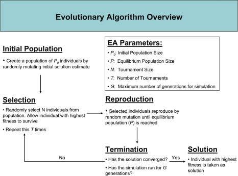
User supplied parameters determine the initial and equilibrium population sizes. During simulation each tournament winner is allowed to have the same number of children that will replenish the population to the equilibrium size. Figure 2 provides an overview of the overall EADRM algorithm.

FIGURE 2:

Evolutionary Algorithm Overview

2.3. Data Simulation and Analysis

A crucial component of any methodological development is the validation of the new method on simulated data. In order to evaluate the potential of EADRM to model both Hill-Slope (sigmoidal) and exponential models of a dose-response, we simulated both types of dose-response models with varying amounts of noise. Unlike in real data applications, by using simulated data with known models, we can evaluate the sensitivity of the method to different parameter settings, and objectively investigate the relative performance of the method, since the true model is known for these simulations. For each combination of model and noise level, 50 simulated datasets were generated for analysis. By performing replicates of each simulated model, the accuracy and precision of the EADRM solutions can be evaluated. This initial round of analysis was to assess how sensitive EADRM is to the configuration parameters. For the sigmoidal models, the four model parameters were randomized and up to +/−10% random noise was added. This randomization was done in a constrained manner to reflect the characteristics of real data. The EC₅₀ was kept between the minimum and maximum concentrations, the E_max was greater than the E_min, the E_min was greater than 0, and the Hill-Slope was between .1 and 8. Each observation generated from these parameters was then given up to +/−10% noise randomly for the evaluation of the performance of the method. For the exponential models, data was generated using the model from [equation 2.1b] with β=1.5 and λ=2.75, with 5% random perturbation added to each datapoint to preclude the chances of an exact fit.

First, the simulated sigmoidal model data (with no noise) was used to evaluate the sensitivity of the EADRM method, in terms of the quality/fit of the solution, convergence rate and computation time. To assess these effects, each configuration parameter was swept over a range of representative values and the convergence rate (the approximate number of generations at which the population of solutions reaches maximal fitness, where there is not improvement in model R² across increasing generations) and the computation time needed to obtain a fit were measured. The configuration parameter evaluation included the following: Initial Population Size, Equilibrium Population Size, and Tournament Size. For each configuration parameter we swept various values for the parameter being tested while the others remain fixed and measured the results. Table 1 summarizes the values used in the parameter sweep. To measure the effect of each configuration parameter, all other configuration parameters not being tested remained constant, and the results were averaged across the simulation replicates for each model simulated.

Table 1:

Evolutionary Algorithm Parameters Evaluated

	Initial Population	Equilibrium Population	Number of Generations	Number of Tournaments	Tournament Size
EA Parameters	5000	200	100	20	10

To select the final configuration parameter values for EADRM, six different permutations were tested on the same data. Since EADRM is a nondeterministic process, each set of configuration parameter values was used to analyze 15 simulated datasets. The model parameter estimates were recorded, and mean value and standard deviation were computed. The optimal configuration parameter settings were determined by these parameter sweep experiments (as described in the results section below) by determing the configuration parameter combinations that resulted in the most accurate and least variant model parameter estimates, with minimal computation time.

To evaluate the potential of EADRM to fit both sigmoidal and exponential data, EADRM was evaluated on simulated data with three settings, that are implemented in the software as user-defined choices. First, on sigmoidal models, EADRM was evaluated by initially generating sigmoidal solutions. Secondly, on the exponential data, EADRM was evaluated by initially generating only exponential solutions. Then, to evaluate the potential of EADRM to evolve appropriate solutions without making any mathematical model assumptions, EADRM was used to model the sigmoidal data by initializing solutions using both the sigmoidal and expontial models.

To compare the performance of EADRM against the traditional NLS approaches, each method was run on simulated sigmoidal data, and results were averaged across the 50 replicates. Initial value selection for NLS was done in the same way as for EADRM as described in Section 2.2.

Finally, to evaluate real world performance each approach was applied to experimental data. Comparisons on real-world concentration-responses were made on mRNA expression data obtain from a quantitative Nuclease Protection Assay (qNPA™) (Roberts et al. 2007) that was run for in-house positive control assays run at CellzDirect. The assay was performed in cultures of primary human Hepatocytes furnished by CellzDirect. The values represent the amount of mRNA expressed by a specific gene quantified by luminescence detection and normalized to the vehicle control (DMSO) to obtain a fold-over-control value. The EA and NLS approaches were applied to these concentration-responses to assess real-world performance. Data from prototypical inducer Rifampicin (RIF) for Cytochrome p450 CYP3A4 was used to evaluate each approach’s performance on a positive response. To evaluate how well negative or suppressed responses were fit, data from chenodeoxycholic acid (CDCA) suppression of the gene 3-hydroxy-3-methylglutaryl-Coenzyme A synthase 2 (HMGCS2) was used. Details of the experiments used for this evaluation can be found in (Roberts et al. 2007).

All test code and simulations were written and conducted using the R Statistical Language (R Development Core Team 2008). Random mutation in the EA and random noise were accomplished using R’s built in random number generator. For comparison, the nls function in R was used, which implements both Gauss-Newton and NL2SOL. Gauss-Newton is the default algorithm and NL2SOL may be used by assigning the algorithm option to “port” in nls. Execution time was measured using R’s system time function (Sys.time()).

All simulations were conducted using a Quad Core Intel® Xeon® E5450, 2x6MB Cache, 3.0GHz, 1333MHz FSB. EADRM code is available from the authors upon request by emailing the corresponding author.

3. RESULTS

In this section we describe the results of the configuration parameter sweep experiments, the evaluation of the performance of EADRM on both sigmoidal and exponential models, the comparison to the NLS results, and the real data application.

3.1. Effect of EA Parameters on Convergence Rate

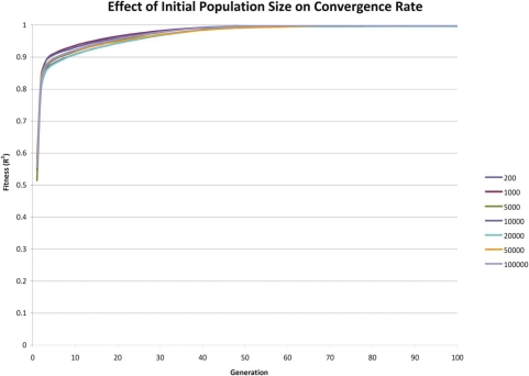
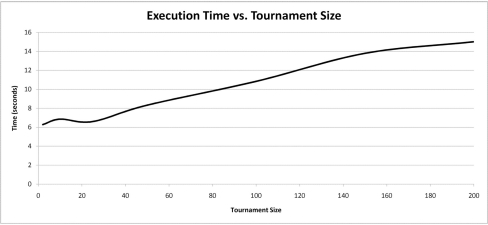
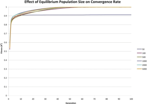
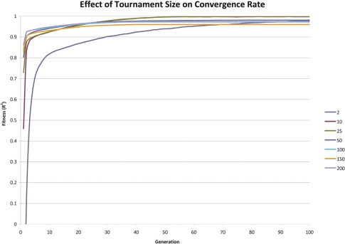
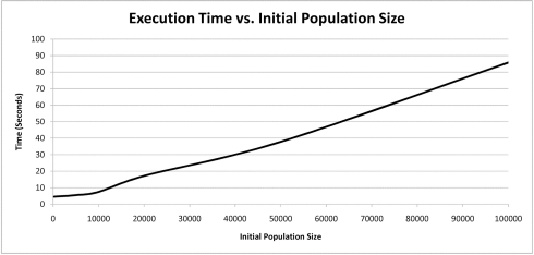
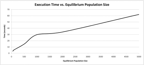
As mentioned above, to evaluate how an individual EADRM configuration parameter affected the convergence rate of the solution, each configuration parameter was modulated while the other three remained fixed. The configuration parameters not being tested were given the values listed in Table 1. Each configuration was then run 50 times and the results averaged as described in Section 2.3. Execution time was also recorded for each configuration and averaged to assess each parameter’s effect. Figures 3 – 8 show these results.

FIGURE 3:

Effect of Initial Population Size on Convergence Rate

FIGURE 8:

Execution Time vs. Equilibrium Population Size

The results indicate that so long as each configuration parameter is reasonably large, the convergence rate is only marginally improved by increasing a given parameter’s size. There is considerable increase in execution time associated with grossly increasing a given configuration parameter’s size. It appears that there is an exponential trade-off between a single configuration parameter’s size and execution time. These simulations suggest that so long as the configuration parameters’ sizes are not cripplingly small, that the convergence rate is roughly similar.

3.2. Selection of Final EADRM Configuration Parameters and Solution Stability Assessment

To select parameter values used in the comparison to the NLS approaches, six configurations representing different permutations of the parameter ranges were simulated to assess how tightly each configuration converged to the same solution. Each configuration was evaluated 15 times and the average and standard deviation for each configuration parameter setting combination was recorded. The six configurations are summarized in Table 2 and the results are tabulated and displayed below in Table 3 and 4. Finally the execution needed for each configuration is summarized in Table 5.

Table 2:

Configuration Parameter Values for Each Combination:

Configuration	1	2	3	4	5	6
Initial Population	5000	20000	5000	5000	20000	10000
Equilibrium Population	200	200	1000	200	5000	1000
Tournament Size	25	25	25	100	500	300

Table showing the different configurations of EA parameters used in simulations.

Table 3:

Average Parameter Values for Each Configuration:

Configuration	Top	Bottom	EC50	W	R2
1	998.699	2.347	0.010004	1.905	0.999779
2	999.125	2.277	0.010015	1.893	0.999859
3	999.506	1.885	0.010018	1.511	0.999976
4	998.726	2.341	0.01001	2.089	0.999768
5	999.615	2.075	0.010005	1.513	0.999997
6	999.38	2.453	0.01001	1.621	0.999925
True Value	1000	1	0.01	1.75

Table showing results from each configuration’s simulations. Each column represents the average value for parameter obtained over 15 simulations of synthetic data with no noise. The true values for each parameter are shown for comparison.

Table 4:

Standard Deviation Values for Each Configuration:

Configuration	Top	Bottom	EC50	W	R2
1	2.569	1.564	5.99E-05	0.864	0.000431
2	2.068	1.525	5.36E-05	1.062	0.000367
3	1.822	1.142	9.81E-05	0.034	0.000014
4	2.951	1.228	4.24E-05	1.226	0.000457
5	0.404	1.079	2.71E-05	0.013	0.000003
6	0.855	1.229	2.36E-05	0.044	0.000785

Standard deviation values were recorded for each configuration to measure each configuration’s stability.

Table 5:

Execution Time for Each Configuration

Configuration	Time (sec)
1	22.62846
2	56.08406
3	468.71754
4	136.27968
5	2581.9843
6	1011.2223

The results show that all configurations, even ones with more modest EADRM configuration parameter values, do relatively well at recovering the true model parameter values and do so in a consistent manner. Configuration combinations 3, 5, and 6 performed the best overall as they had the highest average R², the most accurate average model parameter values, and the lowest average standard deviations. This indicates that these three configuration combinations were able to accurately recover the true model parameters and do so with the least amount of “wobble”. Configuration combination 5 out performed configuration combinations 3 and 6 slightly in nearly all categories at the expense of taking nearly four times the amount of execution time. Given the computational expense of configuration combination 5 in relation to the marginal solution improvement, configuration combination 6 was chosen for use in further analyses. These configuration parameter estimates are recommended for EADRM implementation and application.

3.3. Initial Value Sensitivity

Assessments of the sensitivity to initial model parameter estimates were made on EADRM and the two NLS implementations. The model parameter that caused the most perturbation on final solutions was observed to be the EC50, which represents the curve’s inflection point. To evaluate how much perturbation the initial EC50 estimate influenced the resulting solution, eight different values were given as initial estimates for the EC50 and the results tabulated. NL2SOL and Gauss-Newton advise against running on zero residual data (http://www.R-project.org) so the analysis was run on simulated data with 1% random noise added to each data point. Table 6 shows the curve parameters used during simulation.

Table 6:

Parameter Values

Curve Parameters
EMAX	2256
EMIN	1.064
EC50	1.021
W	2.5165

Using data points generated from the Hill-Slope model defined by the above model parameters, simulations were performed for 8 different initial estimates of the EC50. The results are displayed in Table 7. If an algorithm failed to produce a solution and halted, that is indicated in the table by NA.

Table 7:

Results from Initial Value Simulations

		Initial EC50 Estimate
		0.0001	0.001	0.01	0.1	1	10	100	1000
EA	EMAX	2266.029	2266.724	2266.68	2266.404	2267.874	2267.068	2260.266	2265.44
	EMIN	0.9596	1.0055	1.2661	1.1232	1.0799	0.7031	0.9818	1.023
	EC50	1.0324	1.0325	1.0317	1.0259	1.0309	1.0319	1.0145	1.0279
	W	1.9434	2.0491	1.975	2.0186	2.0207	2.0474	3.7828	2.0268
	R2	0.9999	0.9999	0.9999	0.9999	0.9999	0.9991	0.9998	0.9999
NL2SOL	EMAX	NA	7443	7443	NA	2267.822	NA	NA	3101.499
	EMIN	NA	−7049	−7049	NA	−3.055	NA	NA	785.17
	EC50	NA	0.0039	0.0039	NA	1.029	NA	NA	946.346
	W	NA	−0.0564	−0.0564	NA	1.96	NA	NA	6.471
	R2	NA	0.8356	0.8356	NA	0.9999	NA	NA	0.2182
Gauss-Newton	EMAX	NA	NA	NA	2267.822	2267.822	NA	NA	NA
	EMIN	NA	NA	NA	−3.055	−3.055	NA	NA	NA
	EC50	NA	NA	NA	1.029	1.029	NA	NA	NA
	W	NA	NA	NA	1.96	1.96	NA	NA	NA
	R2	NA	NA	NA	0.9999	0.9999	NA	NA	NA

The results show that for estimates close to the true EC50 value (1.021) the NLS approaches provide very good solutions. However, as the initial model parameter estimate drifts further away from the true value, most often the algorithms are unable to provide a solution at all, and if they do it is generally quite poor. In contrast the EA provides not only a very good solution, but converges to nearly the same solution, independent of the initial model parameter estimate. This result is due to the EA’s considerable robustness and parallel search technique, which keeps it from being pigeon-holed by poor initial model parameter estimates. NLS however relies upon a sequential search and is thus very susceptible to poor initial model parameter values and is reliant upon good initial estimates.

3.4. Performance on Exponential Models

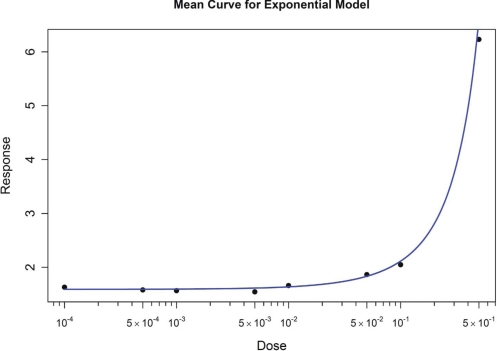
As described above, EADRM was used to evaluate the simulated data generated from an exponential model. Example results are shown in Figure 9. The results are listed in Table 8. The results demonstrate the excellent fit of the models generated by EADRM.

FIGURE 9:

Resulting Fit from Exponential Model

Table 8:

Results from the exponential value simulations.

	B	k
Mean	1.589	2.8497
Standard Deviation	0.108	0.1857
True Value	1.5	2.75

Summary for the parameter estimates averaged across 15 simulations. Includes average parameter estimates, standard deviations, and the true parameter value used to generate the data.

3.5. Performance with No Model Assumptions

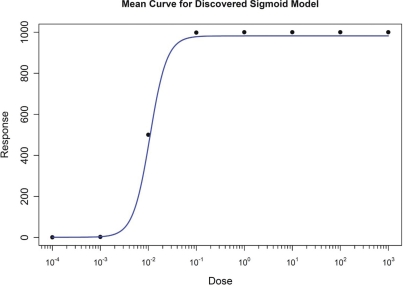
The Hill-Slope simulations were re-evaluated, without using mathematical model assumptions for the initialization, to test the potential of EADRM to evolve not only the model parameter estimates, but also the mathematical model used. The results are shown in Figure 10. Summaries of the results are listed in Table 9. Here we observe that the algorithm was able to correctly fit the data using the Hill-Slope model despite that it was not told explicitly that was the correct model.

FIGURE 10:

Result from Simulating both Exponential and Hillslope individuals on Hillslope Data

Table 9:

Results from the model-free analysis.

	EMAX	EMIN	EC50	W
Mean	982.0656	1.0063	0.108	2.4658
Standard Deviation	85.6183	0.6374	0.0026	1.0338
True Value	1000	1	0.01	2.75

Summary for the parameter estimates averaged across 15 simulations. Includes average parameter estimates, standard deviations, and the true parameter value used to generate the data.

3.6. Performance on Experimental Data

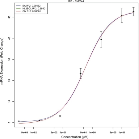
First we present CYP3A4 gene expression data treated with Rifampicin (RIF). This concentration-response represents “flatter” or more-closely linear behavior than do most concentration related gene expression responses. Figure 11 displays this response for all three approaches.

FIGURE 11:

Concentration-Response for CYP3A4/RIF

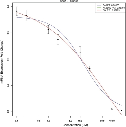
Note that both NLS techniques converge to exactly the same solution and hence both curves are overlaid and only the Gauss-Newton curve remains visible. EADRM produces nearly the exact same solution as NLS but does not underestimate E_min whereas NLS produces an E_min value less than zero. The last response represents a negative or suppression like response of HMGCS2 by CDCA. This is displayed in Figure 12.

FIGURE 12:

HMGCS2 Suppression by CDCA. Note that the green and red lines overlap, and are not distinguishable visually.

4. DISCUSSION AND ANALYSIS

4.1. Examination of the Effect of EA Configuration Parameters on Convergence

Increasing any of the EADRM configuration parameters generally leads to faster solution convergence. However, the configuration parameter that impacted the convergence rate the most was tournament size. Larger tournament size increased the likelihood of picking individuals with higher fitness, and thus increased the rate at which the solution was able to converge. So long as the parameters were sufficiently large, the increase in the rate of convergence was not drastic, however increasing the values of the EADRM configuration parameters did come at a considerable computational cost. In the current implementation the amount of time to perform the simulation is severely affected by an increased equilibrium population size while only yielding marginal increases in convergence rates. This trade-off must be considered in EADRM analysis.

4.2. Stability of EADRM Solutions

As indicated in Section 3.2, the relative stability of the solution produced by EADRM was quite good. All parameters except E_min converged to within 1% of the same value each time. The apparent variation of the derived E_min is not as troubling as one might initially think. Depending on the values for the other parameters we may not have enough evidence to infer the correct value because the minimum observed value may actually be greater than the theoretical E_min. E_min percent errors also suffer from the floor effect. If the true E_min is actually 1 and a value of 1.2 is derived this is a 20% error, however the experimental implications of this error are minute.

4.3. Comparison between EA and NLS and Initial Value Sensitivity

Overall the EA compared very favorably with NLS. In testing, EADRM solutions proved to be more robust, as NLS required specific tuning of the initial values to avoid the errors mentioned previously and considerable effort was given to ensure that NLS would operate in the given input range. In contrast, once the EADRM configuration parameters are set, all that was need were the observations and the concentration/x-axis values. The EADRM was able to take any input range and data shape with out any hand-holding, and minimal model assumptions.

This is of crucial importance to researchers who wish to do truly high-throughput analysis and is indeed the original motivation for this approach. It is this impressive robustness that is EADRM’s strength; one may feed nearly any response and EADRM will optimize the fit based solely on the data without the user having to guess what an appropriate starting point would be.

4.4. Conclusions and Future Directions

While EADRM is still in its infancy, the results of the current study demonstrate that the evolutionary algorithm approach to dose-response modeling is a promising viable alternative to more traditional approaches such as NLS. On both simulated and real data EADRM performed as well as NLS without relying on cumbersome mathematics and avoiding pitfalls such as initial value guesses and search bounds. EADRM was shown to provide the accuracy of the deterministic models with out problems that typically plague such implementations.

Due to the nature of EAs, there are opportunities for massive parallelism in the form of multi-threading. This would decrease the time needed to run a simulation drastically and allow the values of the EADRM configuration parameters to be increased, which would in turn increase convergence rate thus decreasing the number of generations needed for a given simulation. Additional aspects of the evolutionary process should be also be evaluated within the EADRM approach. The addition of crossover operators, different models of parallelization, etc should be investigated for their impact on EADRM performance.

Other improvements may also be made by exploring different statistical criteria for fitness and for model selection. Currently we have used R² as our fitness criterion because it is familiar and adapts well across different types of models. However, it may be that other fitness functions could improve the solution quality. Also, we currently take the individual who has the highest fitness as the winner, without taking model complexity into consideration. Future directions may include accounting for model complexity when deciding between populations containing different types of models.

Finally, as our method is proposed for application to high-throughput dataset, computation time should be optimized, including the incorporation of in line C code to speed up the analysis run-time and parallelization, and competitive run times with conventional methods should be evaluated. Because the NLS approaches implemented in the current study are sequential, and incorporate in line C code and rely on “recipes” from “numerical cook books, a fair computational comparison is not possible in this early stage of EADRM development, and the implementation of the NLS methods is substantially faster than EADRM. With continued development, the EADRM approach can be optimized for more comparable run-times.

FIGURE 4:

Effect of Equilibrium Population Size on Convergence Rate

FIGURE 5:

Effect of Initial Tournament Size on Convergence Rate

FIGURE 6:

Execution Time vs. Initial Population Size

FIGURE 7:

Execution Time vs. Equilibrium Population Size

REFERENCES

- Bates DM, Watts DG. Nonlinear Regression, Analysis and its Applications. John Wiley; New York: 1988. [Google Scholar]
- Björck A. Numerical methods for least squares problems. SIAM; Philadelphia: 1996. [Google Scholar]
- Chamjangali MA, Beglari M, Bagherian G. Prediction of cytotoxicity data (CC50) of anti-HIV 5-pheny-l-phenylamino-1H-imidazole derivatives by artificial neural network trained with Levenberg-Marquardt algorithm. J of Molecular Graphics and Modelling. 2007;26(1):360–367. doi: 10.1016/j.jmgm.2007.01.005. [DOI] [PubMed] [Google Scholar]
- Delahaye D, Puechmorel S. Air Traffic Controller Keyboard Optimization by Artificial Evolution. Lect Not Comp Sci. 2004;2936:177–188. [Google Scholar]
- Dennis JE, Gay DM, Welsch RE. Algorithm 573. NL2SOL — An adaptive nonlinear least-squares algorithm, ACM Trans. Math. Software. 1981;7:369–383. [Google Scholar]
- Fogel LJ, Owens AJ, Walsh MJ. Artificial Intelligence through Simulated Evolution. Wiley; New York: 1966. [Google Scholar]
- Hariparsad N, Brian CA, Evers R, Chu X. Comparison of Immortalized Fa2N-4 Cells and Human Hepatocytes as in Vitro Models for Cytochrome P450 Induction. Drug Metabolism and Desposition. 2008;36:1046–1055. doi: 10.1124/dmd.108.020677. [DOI] [PubMed] [Google Scholar]
- Holland JH. Adaptation in natural and artificial systems: an introductory analysis with applications to biology, control, and artificial intelligence. University of Michigan Press; Michigan: 1975. [Google Scholar]
- Knowles J, Corne D, Kalyanmor D. Multiobjective Problem Solving from Nature. Springer; New York: 2008. [Google Scholar]
- Koza J. Genetic Programming. MIT Press; Cambridge: 1995. [Google Scholar]
- Moore JH, Parker JS. In: Evolutionary computation in microarray data analysis In: Methods of Microarray Data Analysis. Lin S, Johnson K, editors. Kluwer Academic Publishers; Boston: 2001. [Google Scholar]
- Motsinger AA, Hahn LW, Dudek SM, Ryckman KK, Ritchie MD. Alternate Cross-Over Strategies and Selection Techniques for Grammatical Evolution Optimized Neural Networks. Proc. of the 8th Ann Conf on Genetic and Evolutionary Comp. 2006;1:947–948. doi: 10.1145/1143997.1144163. [DOI] [PMC free article] [PubMed] [Google Scholar]
- Motsinger-Reif AA, Reif DM, Fanelli TJ, Ritchie MD. A comparison of analytical methods for genetic association studies. Genetic Epidemiology. 2008;32:325–340. doi: 10.1002/gepi.20345. [DOI] [PubMed] [Google Scholar]
- Motsinger-Reif AA, Ritchie MD. Neural networks for genetic epidemiology: past, present, and future. BioData Min. 2008;171(1):3. doi: 10.1186/1756-0381-1-3. [DOI] [PMC free article] [PubMed] [Google Scholar]
- National Institutes of Health Chemical Genomics Center Assay Guidance Manual. 2008. Available at: http://www.ncgc.nih.gov/guidance/section3.html#models-guides.
- Oyama A, Liou M. Multiobjective Optimization of Rocket Engine Pumps Using Evolutionary Algorithm. National Aeronautics and Space Administration, Glenn Research Center; Hanover MD: 2001. [Google Scholar]
- Pinheiro JC, Bretz F, Branson M. Dose Finding in Drug Development, Chapter 10. Springer; New York: 2006. [Google Scholar]
- R Development Core Team . R: A language and environment for statistical computing. R Foundation for Statistical Computing; Vienna, Austria: 2008. URL http://www.R-project.org. [Google Scholar]
- Roberts RA, Sabalos CM, LeBlanc ML, Martel RR, Frutiger YM, Unger JM, Botros IW, Rounseville MP, Seligmann BE, Miller TP, Grogan TM, Rimsza LM. Quantitative nuclease protection assay in paraffin-embedded tissue replicates prognostic microarray gene expression in diffuse large-B-cell lymphoma. Lab Invest. 2007;87:979–9. doi: 10.1038/labinvest.3700665. [DOI] [PubMed] [Google Scholar]
- Rolls ET, Treves A. Neural Networks and Brain Function. Oxford University Press; Oxford: 1998. [Google Scholar]
- Schnell S, Grima R, Maini PK. Multiscale Modeling in Biology, American Scientist. 2007;95:134–142. [Google Scholar]
- Vanden Heuvel JP, Clark GC, Bell DA, et al. Dioxin-responsive Genes: Examination of Dose-Response Relationships Using Quantitative Reaction. Cancer Research. 1994;54:62–68. [PubMed] [Google Scholar]