Simultaneous recognition and segmentation of cells: application in C.elegans

Abstract

Motivation: Automatic recognition of cell identities is critical for quantitative measurement, targeting and manipulation of cells of model animals at single-cell resolution. It has been shown to be a powerful tool for studying gene expression and regulation, cell lineages and cell fates. Existing methods first segment cells, before applying a recognition algorithm in the second step. As a result, the segmentation errors in the first step directly affect and complicate the subsequent cell recognition step. Moreover, in new experimental settings, some of the image features that have been previously relied upon to recognize cells may not be easy to reproduce, due to limitations on the number of color channels available for fluorescent imaging or to the cost of building transgenic animals. An approach that is more accurate and relies on only a single signal channel is clearly desirable.

Results: We have developed a new method, called simultaneous recognition and segmentation (SRS) of cells, and applied it to 3D image stacks of the model organism Caenorhabditis elegans. Given a 3D image stack of the animal and a 3D atlas of target cells, SRS is effectively an atlas-guided voxel classification process: cell recognition is realized by smoothly deforming the atlas to best fit the image, where the segmentation is obtained naturally via classification of all image voxels. The method achieved a 97.7% overall recognition accuracy in recognizing a key class of marker cells, the body wall muscle (BWM) cells, on a dataset of 175 C.elegans image stacks containing 14 118 manually curated BWM cells providing the ‘ground-truth’ for accuracy. This result was achieved without any additional fiducial image features. SRS also automatically identified 14 of the image stacks as involving ±90^○ rotations. With these stacks excluded from the dataset, the recognition accuracy rose to 99.1%. We also show SRS is generally applicable to other cell types, e.g. intestinal cells.

Availability: The supplementary movies can be downloaded from our web site http://penglab.janelia.org/proj/celegans_seganno. The method has been implemented as a plug-in program within the V3D system (http://penglab.janelia.org/proj/v3d), and will be released in the V3D plugin source code repository.

Contact: pengh@janelia.hhmi.org

1 INTRODUCTION

One of the promises of bioimage informatics is to quantitatively measure and accurately target single cells, thus facilitating improved throughput for genetic and phenotypic assays (Peng et al., 2008). A number of 3D cell and gene expression image segmentation, recognition and tracking techniques have been developed and applied to widely used model animals, including Caenorhabditis elegans (Bao et al., 2006; Jaensch et al., 2010; Long et al., 2008, 2009), fruit fly (Fowlkes et al., 2008; Luengo Hendriks et al., 2006; Zhou and Peng, 2007) and zebrafish (Keller et al., 2008). Caenorhabditis elegans is well known for its invariant lineage and the unique identities of its cells. Single-cell image recognition and tracking techniques for this animal have led to a deeper understanding of the genetic signatures of cells, and the relationship between cell lineage and cell types (Bao et al., 2006; Liu et al., 2009; Murray et al., 2008). This article focuses on a new method for recognizing and segmenting C.elegans cells that is more reliable and applicable to more sample protocols.

Existing image analysis pipelines for single-cell resolution studies typically start with a segmentation of the cells in a 3D image, followed by an ad hoc recognition or tracking process. It is typically hard to ensure an error-free segmentation of cells in an image sample, especially when (i) the image has an uneven background or low signal to noise ratio, or (ii) nuclei are so crowded as to touch each or have irregular morphology. Our experience (Long et al., 2009) is that segmentation errors promote errors in the subsequent recognition task in a non-additive fashion. In addition, within this previous framework, useful prior information, such as the relative location relationship of cells, and useful statistics from the recognition phase, such as discrepancies between the predicted and a priori cells locations, are hard to incorporate in a way that improves the overall analysis.

In addition, for a variety of experimental settings, it may be difficult to generate some of the currently used fiducial image features that are critical for accurately recognizing cells. For example, in the L1 larval stage of C.elegans, there are 81 body wall muscle (BWM) cells. These cells form four nearly symmetrical bundles, each of which has 20 or so cells in one of the ventral-left, ventral-right, dorsal-left and dorsal-right quadrants. Recognizing these BWM cells is critical because they can serve as additional fiducial points for recognizing other cells in the animal. In experiments using fixed animals (e.g. Long et al., 2009) that also stain all nuclei, one can recognize these four bundles based on the asymmetry of the distribution of other cells (e.g. the 15 ventral motoneurons forms an almost linear array along the ventral side of the animal). Nonetheless, for live animal experiments, due to the cost of building transgenic animals and the limited number of fluorescent color channels, it is desirable to be able to recognize these BWM cells or other cells (e.g. intestinal cells and neurons) directly without additional fiducial patterns.

In this article, we propose a new approach to recognize and segment cells in C.elegans. We essentially eliminate the need for a two-step, segment-then-recognize process. Instead, our method recognizes cells directly, producing the segmentation as a by-product. We realize this idea as an atlas-guided voxel classification algorithm, which integrates the processes of atlas-to-image mapping and voxel classification under a robust deterministic annealing framework. We have experimentally tested the performance of the new approach on datasets of BWM cells and a number of other cell types. Our approach generalizes well in producing reasonable automatic recognition accuracy for 14 118 manually curated cells.

2 ATLAS-TO-IMAGE MATCHING

The input of our algorithm consists of a 3D image stack where the target cells have been stained in a single color channel, and a 3D atlas (which is a 3D point cloud representing the stereotyped spatial locations) of the target cells. The goal of the algorithm is to automatically extract the ‘meaningful’ objects in the image and assign one of the cells in the atlas to each of these objects. The atlas is produced in our previous study (Long et al., 2009).

Mathematically, suppose we have an image that consists of N voxels V={v_i, i=1, 2,…, N} and an atlas of K cells C⁰={c_j⁰, j=1, 2,…, K}, where v_i is the i-th voxel and c_j⁰ is the j-th cell, respectively. The goals of our algorithm are (i) to classify (i.e. label) the voxels X into K groups, each of which corresponds to a unique cell, and at the same time (ii) to smoothly map each atlas cell c⁰_j to a new 3D spatial location in the image that can best represents the corresponding voxel subset.

One intuitive and conventionally used method is to first segment all image objects, and then use certain matching methods, such as the bipartite graph matching or the constrained graph matching to assign the identities (Long et al., 2008). One drawback of this method is that the over- or under-segmentation of cells will affect the recognition.

We consider a direct atlas-to-image matching approach, to attain both recognition and segmentation of cells at the same time. Since the atlas encodes all target cells' identities and their spatial location relationship, our method recognizes cells via smoothly deforming the atlas to fit the image. This process effectively classifies, or labels, voxels in the image; each group of voxels with the same label represents the extraction of a ‘meaningful’ object and thus the image is also segmented. From a segmentation perspective, the key difference between our new approach and previous ones is that now we can naturally incorporate the relative location relationship of cells that is encoded in the cell atlas when we segment cells, thus reducing the chance of wrong segmentation. More importantly, with the new approach we could directly predict cell identities, without the complication due to problematic segmentation. We call this new atlas-guided voxel classification approach the simultaneous recognition and segmentation (SRS) of cells.

Our approach can be viewed as a substantial extension of a point-set matching method based on deterministic annealing (Chui and Rangarajan, 2000). Our SRS method not only extends the deterministic annealing approach to the 3D image domain (Sections 3.1 and 3.2), but also proposes a systematic way to incorporate the domain prior information of cells' spatial distribution to solve real cell annotation and segmentation problems (Section 3.3).

3 SRS ALGORITHM

There are two aspects in the SRS algorithm, namely (i) given an atlas of cells, how to label/classify voxels, (ii) how to geometrically transform the 3D atlas of cells. We formulate the following mathematical model to address both of them.

3.1 Iterative voxel classification

Let us first assume the availability of a spatial geometric transform f(.) (Section 3.2), the deformed atlas can be written as C={c_j, j=1, 2,…, K}, where each c_j=f(u_j, C⁰) and u_j is an auxiliary variable [Equation (3)]. The task is to assign a cell label to each voxel so that each subgroup of voxels sharing the same label can well represent the respective cell, and thus overall the image best fits the deformed atlas.

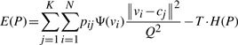
We consider P=[p_ij], where p_ij∈[0, 1], which is the classification probability of the i-th voxel to the j-th cell. Apparently for any i∈[1, N], Σ_jp_ij=1. We formulate the following ‘cost’ function:

(1)

where Ψ(v_i)=255 − I(v_i) is the inversed image voxel intensity that is used to penalize the assignment on the low intensity voxels (assume we have 8-bit images where the maximal intensity is 255), Q equals the maximum of the three dimensions of the image and is used to normalize the distance of a voxel and a mapped cell, H(P)=−Σ_iΣ_jp_ijlog(p_ij) is the aggregated entropy function of the classification matrix P, and T≥0 is a varying temperature factor (see discussion below).

Equation (1) consists of two competing terms. Minimizing Equation (1) is equivalent to minimizing the first term while maximizing the second term. Minimizing the first term means for bright voxels assigning large classification probability to their closest cells. As a result, the classification probability matrix should be far away from uniform distribution. Maximizing the second term means the voxel classification probability should distribute as evenly as possible. How to find a good balance of these two terms?

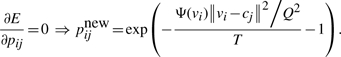
We consider the time-varying temperature, T, as a way to smoothly tune the balance of the two terms in Equation (1) during the optimization. We choose the initial value of T to be a large positive number. Indeed, when E(P) is a local optimum, for any i, j values we will have

(2)

Therefore, if we use Equation (2) as the formula to iteratively update p_ij (of course p_ij will then be normalized in every iteration, so that for any i∈[1, N], Σ_jp_ij=1), a large T value means that p_ij will be almost uniformly distributed, thus H(P) has a value close to its maximum.

On the other hand, at the end of the optimization, the cell locations in the atlas should optimally represent all image voxels. This can be implemented by choosing T=0. We eliminate the influence of the second term by gradually decreasing T to 0 over iterations: T=20×0.95ⁿ, where n=0, 1, 2,…, is the iteration number.

During the iterative optimization, we also update the location of each cell c_j (j=1,…, K) by using the spatial transform f(.) on the weighted center of the mass of all voxels,

(3)

Of note, we do not need to segment all cells explicitly during iterations. However, whenever an explicit segmentation of all cells is needed, we can determine the best cell that contain a voxel v_i by computing argmax_j p_ij. The segmentation mask of a cell c_j consists of all voxels that are optimally contained in c_j.

In 3D microscopic images, the total number of voxels, N, can easily exceed tens or hundreds of millions. However, the real image objects (e.g. cells) typically only occupy a small portion of the image volume in the ‘foreground’ area. There is also a strong correlation of intensity of the spatial nearby voxels. Therefore, to speed-up the iterative voxel classification, we first down-sample an image by a factor (typically 4) for each of the X, Y and Z dimensions to reduce the number of voxels. We use the ‘averaging’ filter in down-sampling, thus the image voxel intensity used is smoother than the original image; as a result, the voxel classification is more robust to noise. In addition, we use a conservative threshold, which is the mean intensity of the image plus one or two times of the standard deviation of the all image voxels' intensity, to define the ‘foreground’ of an image. We run SRS only on the foreground area to produce the result more swiftly. We produce the final classification or segmentation results by up-sampling the intermediate result on the down-sampled image to have the same dimensions of the original input image.

3.2 Spatial transform

Why we need a specially designed spatial transform f(.)? The reason is that if we do not use it, which means that c_j^new=u_j, i.e. there is no constraint of the cell deformation, cells may switch their relative locations in the 3D space. This spatial distortion is meaningless, as most cells' relative locations are preserved from animal to animal (Long et al., 2009).

To preserve the relative locations of cells encoded in the initial atlas C⁰, one may use a simple 3D affine transform, which can translate, scale, shear and rotate the atlas. It is well known that an affine transform preserves the collinearity of points, and also the ratios of the distances of distinct points on a line. However, using the affine transform corresponds to dropping u_j from Equation (3). One obvious caveat is that when the cell locations in the image data of an actual animal sample differ from the ‘standard’ locations in the atlas, the affine transform cannot map all cells' locations in the atlas exactly to those in the actual image.

To allow local deformation but also preserve cells' relative locations and global smoothness, we consider the smoothing-thin-plate-spline (STPS) (Wahba, 1990) transform. STPS can be decomposed into an affine transform and a weight-factor controlled non-linear non-affine warping component.

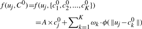
Given two corresponding point sets {c_j⁰, j=1, 2,…, K} and {u_j, j=1, 2,…, K} that represent the 3D locations of cells in the initial atlas and the locations of subgroups of voxels in each iteration [as in Equation (3)], a STPS transform f(u_j, C⁰) has the following form,

(4)

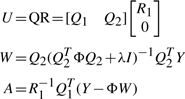
where A is an affine transform matrix, ω_k is the non−affine deformation coefficient, ϕ(r)=r²log(r) is the STPS kernel function. Denote W=[…,ω_k,…]^T, U and Y as the concatenated version of points' coordinates u_j and the initial coordinate c_j⁰, we compute the least square solution for STPS parameters A and W using QR factorization (Wahba, 1990):

(5)

where Q, R, Q₁, Q₂ and R₁ are the QR factorization matrices (and submatrices) of U, Φ is a K×K matrix, where its (i, j)-th element equals ϕ(||c_i⁰−c_j⁰||), and λ>0 is a weight that balances the affine portion and non-affine portion of STPS. When λ≫1, elements in W will be close to 0, thus the affine part dominates Equation (4).

Since we use iterative optimization to evolve the cell atlas, for every iteration, once we have obtained the matrix U using Equation (3), we then calculate W and A using Equation (5), followed by producing a smoothly deformed new cell atlas using Equation (4).

Of note, we can also tune the value of λ so that the spatial transform f(.) exhibits different levels of the deformation. This helps fit the image best to the deformed atlas, while keeping the global smoothness and cells' relative location relationship. We implement this by setting λ=5000 and over iterations gradually decreasing the value as λ=5000×0.95ⁿ, where n=0, 1, 2,…, is the iteration number.

3.3 Using cells distribution in the atlas

The atlas-to-image matching method discussed in Sections 3.1 and 3.2 has not considered the intrinsic spatial distribution of cells in an atlas. A biological model system typically has different levels of invariant features along its ‘major’ axes. For C.elegans, the greatest degree of freedom of cell locations is along the animal's anterior–posterior (AP) axis; there is a general symmetry of cell distribution along left–right (LR) axis, but along the dorsal–ventral (DV) axis there is also an obvious asymmetry if all cells are considered. However, the variation of cell location along DV- or LR-axes is far less than that along the AP axis. When the BWM cells are considered, typically they form four almost symmetrical bundles in both LR and DV directions, except at the tail region of the animal.

Hence, we added an anisotropic weight function D(.) in the cost function in Equation (1) to give a weaker penalty to the variation along the AP axis than those along the DV- and LR-axes:

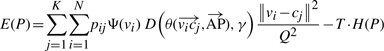(6)

where θ(.) is the angle between the vector from v_i to c_j and the AP axis of the animal. The weight function D(θ, γ) has the following form,

(7)

where γ≥1 is the coefficient of a raised cosine function that controls the degree of cells' movement along the AP direction (we set γ=3), and λ^ani is a threshold (typically λ^ani=20) that is related to λ in Equation (5). When λ>λ^ani, cells in the atlas span as broadly as possibly across the image pattern; when λ≤λ^ani, the anisotropic deformation is enabled and thus cells move primarily along the AP axis.

When only a subset of cells (e.g. BWM cells) is considered, the symmetry of these cells may make it hard to recognize them. For instance, during the atlas-to-image matching, an entire bundle of BWM cells may switch their locations with another bundle, thus both bundles would be wrongly recognized in this case. To prevent this ‘mirroring’ error, we considered the affine transform A in Equation (5). In 3D, A is a 4×4 matrix, of which the top-left 3×3 submatrix, denoted as L, can be used to prevent the wrong ‘mirroring’ (i.e. reflection transform) when we constrain its determinant to be greater than 0. Of note, this suppression of the reflection transform does not only prevent inter-bundle mirroring error, but also allow 180^○ rotation that indeed consists of two consecutive reflection transforms.

In our implementation to both prevent mirroring and allow 180^○ rotation, we compute the standard singular value decomposition (SVD) of L and obtain its three singular-values, d₁, d₂ and d₃. If a reflection, i.e. det(L)<0, is detected, we replace d₃ with −d₃, re-compute L using the new d₃ value (and also with other ‘old’ components obtained in the SVD), and then use the new L matrix to replace the top-left 3×3 submatrix in A.

Theoretically, the only remaining difficulty in recognizing symmetrical subsets of cells is when they are not only symmetrical in both DV and LR directions, but also have identical locations (along AP axis) in adjacent bundles of cells that are 90^○ apart. We should note that this case is indeed very rare biologically; for example, C.elegans BWM cells do not really have this ‘90^○ similarity’. However, due to imperfect staining or partial image data (e.g. the unsimilar region is not imaged or is contaminated by noise), it may still be observable in real data.

We detect the potential ±90^○ rotation around the AP axis (which corresponds to the x-axis in our C.elegans image data) in atlas-to-image matching using the following method. We note that using SVD the affine transform matrix A can be written as A=R₁(R₂⁻¹DR₂), where R₁, R₂ are rotation matrixes and D is the singular value matrix. The matrix R₁ controls the ‘final’ rotation of the atlas, and indeed it can also be viewed as a sequential rotation around the x-, y- and z-axes. The rotation angle around x-axis is α=arctan(R₁(2, 3)/R₁(3, 3)), where R₁(i, j) is the element at the i-th row and the j-th column of R₁. Whenever |α| is >45^○, there is a potentially erroneous ±90^○ rotation. Finally, once an image is detected to have a ±90^○ rotation around the AP axis, we can always pre-rotate either the atlas or the image 90^○ around the AP axis and then use SRS again to make a prediction, as SRS is able to correct the 180^○ mismatch between the atlas and the image (as explained in the middle of this section).

4 EXPERIMENTAL RESULTS

4.1 Data and parameters

We tested the SRS algorithm using 3D confocal image stacks of the L1-stage of C.elegans (Liu et al., 2009). In all the images, 81 BWM and 1 depressor muscle cell (DEP) are labeled using myo3::GFP. We straightened all these images (Peng et al., 2008) before applying the SRS method to them.

For all experiments in this article, we stop the iterative optimization when λ becomes to be less than λ^ani [in Equation (7)] and the sum of the location change of all cells between two consecutive iterations is <0.1 voxel. Typically SRS converges within about 200 iterations.

4.2 Visual inspection of the SRS process

Figure 1 and the supplement movie illustrate the process of SRS for a hard example where the initial atlas has a 180^○ rotation with to the subject image. The initial locations of cells in the atlas obviously mismatch the image objects along AP-, DV- and LR-axes.

Fig. 1.

Simultaneous cell recognition and segmentation. In each image, the red spheres show the deformed atlas; the segmented pixels and their corresponding cells in the atlas are connected by lines with different colors. The first row shows the original image overlaid with the initial atlas; other rows show results of several intermediate steps of the iterative optimization, with which the atlas of cells (BWM cells shown here) deform to the optimal locations and the foreground image voxels are automatically classified to (and thus segmented) each of these cells. The energy values shown are normalized using the total number of image foreground voxels. When we produced this figure, the image intensity was enhanced for better visibility. The surface rendering of the segmented regions can be seen in Figure 5.

Over a series of iterations, image voxels are assigned to the cells gradually until convergence of the cost function, that decrease from 144 to 9.9. Initially, e.g. iteration 3, the segmentation is very inaccurate. However, at this stage due to the high temperature in Equation (1), the aggregated entropy function term plays the major role. This indeed helps the atlas rotate 180^○ to fit to the image. Then when the temperature is cooled (iterations 10−20) and λ>λ^ani, the affine transform plays a major role in deforming the atlas. When the temperature gets even lower (iterations 20 onward), the local adjustment of voxel assignments becomes the major factor to further decrease the deformation of the atlas and best fit the cells in the atlas to the centers of their respective image objects. A group of voxels that correspond to the optimal fit of an atlas cell form a natural segmentation mask of this cell in the image.

4.3 Robustness of SRS

We randomly selected four images (first row of Fig. 2a and second rows of Fig. 2b–d) that have different levels of variations in their scales, rotations, noise levels and cell distributions. For instance, the cell distribution in the tail region indicates that the worm in (Fig. 2c) has a different orientation from those in Figure 2a–d.

Fig. 2.

Robustness of the SRS algorithm. For YZ plane and XY plane, the maximum intensity projections are shown. For each subfigure, the deformed atlas (red spheres) was also overlaid on the respective volumetric image for better visualization. For (b– d), the image intensity was also enhanced for more visible display only. For (a– d), all SRS results were produced using the original intensity-unenhanced images.

The SRS algorithm is able to robustly deform the same initial atlas to all of four images and correctly recognize all BWM and DEP cells (last rows of Fig. 2 subfigures). These 3D images and their deformed atlases, as well as the full-resolution movies of the optimization process can be found in our online supplement.

4.4 Consistency of SRS

We started from different initial atlas orientations and investigated the consistency of the results produced by the SRS method. For each of the four images in Figure 2, we rotated the cell atlas around its AP axis every 45^○ in the range of [0, 360) degrees to produce eight different initializations, each of which was then deformed to the respective image. For each group of eight deformed atlases, we calculated the average and maximum root mean square error (RMSE) of their corresponding cell positions, as an indication of the consistency of these results.

Table 1 shows that all the RMSE scores are much smaller than one pixel, even for the cases where the initial atlas had an orientation that was 180^○ from the ‘true’ orientation. This demonstrates that the SRS algorithm is able to effectively adjust the cells' location for these image examples. Both the test images and the rotated atlases are available in the online supplements.

Table 1.

Consistency of the SRS results for different initializations

Image score	Maximal RMSE (pixel)	Average RMSE (pixel)
1	1.019e-05	6.448e-06
2	1.019e-05	7.107e-06
3	1.051e-05	6.192e-06
4	1.058e-05	6.421e-06

4.5 Accuracy of SRS

We used a large dataset of 175 image stacks to evaluate the recognition accuracy of SRS. In this dataset, there are a total of 14 118 BWM and DEP cells that were carefully annotated by an expert of C.elegans anatomy and thus were used as the ‘ground-truth’ identities of cells in our study.

Because the ground-truth location of a cell determined by the expert could deviate from the one that is automatically predicted by SRS, we deem a cell to be ‘correctly’ recognized if (i) the SRS prediction of a cell is the spatially nearest match of this cell's ground-truth location, compared with all other cells' ground-truth locations, and (ii) the Euclidean distance between the SRS prediction and the respective ground-truth location is not larger than 8 voxels, which approximately equal the radius of a typical cell along AP axis.

For the 175 stacks, SRS automatically identified 14 stacks involving ±90^○ rotations that may contain less optimal cell prediction. In the remaining 161 stacks, there are 12 976 cells. SRS correctly predicted the identities of 12 863 cells (99.13% recognition rate). When we forced SRS to predict all stacks (including the 14 less optimal ones), the overall recognition rate is 97.7%. These results indicate SRS is highly effective.

A closer look at the recognition accuracy for each of the 82 BWM and DEP cells (Fig. 3) shows that most cells can be recognized with accuracy better than 97%, except the cell BWMDL23 in the dorsal-left side of the worm. We checked the original images where this happened and found that indeed this was due to an additional and nearby Sphincter muscle (SPH) cell that is not in our atlas, but also has weak expression in some of the original images, influencing the recognition.

Fig. 3.

Average recognition rates of individual BWM and DEP cells using 161 image stacks.

4.6 Recognition of other cells

To illustrate the general usability of our method, we also applied it to other cell types. Figure 4 demonstrates that for a stack of intestinal cells where there are 20 nuclei (labeled using C26B9.5::wCherry using a similar protocol of the BWM cell labeling), SRS is able to predict the identities of all nuclei, while at the same time segment all of them, even some of the nuclei are relatively dark.

Fig. 4.

SRS results on recognition of 20 intestinal cells (labeled by C26B9.5::wCherry). SRS was applied to the original image to produce the results in the third and fourth rows simultaneously. The second row shows the contrast-enhanced image for illustration purpose, especially to visualize four posterior nuclei.

4.7 Comparison with other methods

We also compared SRS with previous segmentation and recognition methods. The watershed algorithm is one of most popular methods used in 2D or 3D cell segmentation. We compared with the shape-based watershed algorithm, which is typically thought to be a well-performing method when the image intensity is uneven (such as our test images). To produce the best possible watershed result, we tried multiple different thresholds to define image foreground and multiple Gaussian smoothing kernels to remove image noise. Note that for SRS, we did not do these preprocessing. However, Figure 5 shows that compared with SRS, in the best case the watershed result still has substantial over-segmentation and under-segmentation. Of note, previous studies (e.g. Long et al., 2009) may use additional methods to split or merge cells after the initial watershed segmentation. SRS avoids these extra steps.

Fig. 5.

Comparison of the segmentation results of watershed and SRS. The same test image in Figure 1 was used. The first, second and third row in (a–c) show the original image, watershed and SRS segmentation result respectively. The color-surface objects indicate the different segmentation regions. In head and tail region zoom-in view (b and c) yellow arrow: over-segmentation; red arrow: under-segmentation.

In Section 2, we discussed that SRS could be thought as an extension of a deterministic annealing point-cloud matching. Obviously, such a point-cloud method cannot be directly applied to the image domain. Therefore, we compared the previous deterministic annealing method [using the software in Chui and Rangarajan (2000)] by setting its input to be the expert-curated segmentation that does not have any segmentation error. For the test image in Figure 1, we found that deterministic annealing will produce 180^○ rotated results and thus 78 of the 82 stained cells were wrongly recognized. For the 175 images in our dataset, the average recognition rate of deterministic annealing (with manually produced ‘perfect’ segmentation) was 49.03% for all 14 118 stained cells. The main reason is that nearly half of images in our dataset are 180^○ rotated compared with the atlas. Chui's method cannot deal with this kind of big rotation, even with the ‘ideally’ segmented point clouds. Thus, SRS is more suitable for the application in this article.

5 DISCUSSION AND CONCLUSION

In this article, we present a highly effective method to simultaneously recognize and segment 3D cellular images. We also successfully applied it to automatically annotate C.elegans BWMs and intestinal cells. We are currently testing this method for other cell types in C.elegans. This method has potential to be applied to other model systems, such as fruit fly. It may also be used as an automatic 3D image registration method to recognize spatially distinctive feature points: for example, we plan to use it to enhance our 3D BrainAligner program (Peng et al., 2011).

REFERENCES

- Bao Z., et al. Automated cell lineage tracing in Caenorhabditis elegans. Proc. Natl Acad. Sci. USA. 2006;103:2707–2712. doi: 10.1073/pnas.0511111103. [DOI] [PMC free article] [PubMed] [Google Scholar]
- Chui H., Rangarajan A. A new algorithm for non-rigid point matching. IEEE Conf. Comput. Vision Pattern Recogn. 2000;2:44–51. [Google Scholar]
- Fowlkes C., et al. A quantitative spatiotemporal atlas of gene expression in the Drosophila blastoderm. Cell. 2008;133:364–374. doi: 10.1016/j.cell.2008.01.053. [DOI] [PubMed] [Google Scholar]
- Jaensch S., et al. Automated tracking and analysis of centrosomes in early Caenorhabditis elegans embryos. Bioinformatics. 2010;26:i13–i20. doi: 10.1093/bioinformatics/btq190. [DOI] [PMC free article] [PubMed] [Google Scholar]
- Keller P.J., et al. Reconstruction of zebrafish early embryonic development by Scanned Light Sheet Microscopy. Science. 2008;322:1065–1069. doi: 10.1126/science.1162493. [DOI] [PubMed] [Google Scholar]
- Liu X., et al. Analysis of cell fate from single-cell gene expression profiles in C. elegans. Cell. 2009;139:623–633. doi: 10.1016/j.cell.2009.08.044. [DOI] [PMC free article] [PubMed] [Google Scholar]
- Long F., et al. Automatic recognition of cells (ARC) for 3D images of C. elegans. Lect. Notes Comput. Sci. Res. Comp. Mol. Biol. 2008;4955:128–139. [Google Scholar]
- Long F., et al. A 3D digital atlas of C. elegans and its application to single-cell analyses. Nat. Methods. 2009;6:667–672. doi: 10.1038/nmeth.1366. [DOI] [PMC free article] [PubMed] [Google Scholar]
- Luengo Hendriks C.L., et al. 3D morphology and gene expression in the Drosophila blastoderm at cellular resolution I: data acquisition pipeline. Genome Biol. 2006;7:R123. doi: 10.1186/gb-2006-7-12-r123. [DOI] [PMC free article] [PubMed] [Google Scholar]
- Murray J.I., et al. Automated analysis of embryonic gene expression with cellular resolution in C. elegans. Nat Methods. 2008;5:703–709. doi: 10.1038/nmeth.1228. [DOI] [PMC free article] [PubMed] [Google Scholar]
- Peng H., et al. Straightening C. elegans images. Bioinformatics. 2008;24:234–242. doi: 10.1093/bioinformatics/btm569. [DOI] [PMC free article] [PubMed] [Google Scholar]
- Peng H., et al. V3D enables real-time 3D visualization and quantitative analysis of large-scale biological image data sets. Nat. Biotechnol. 2010;28:348–353. doi: 10.1038/nbt.1612. [DOI] [PMC free article] [PubMed] [Google Scholar]
- Peng H., et al. BrainAligner: 3D registration atlases of Drosophila brains. Nat. Methods. 2011;8:493–498. doi: 10.1038/nmeth.1602. [DOI] [PMC free article] [PubMed] [Google Scholar]
- Wahba G. Spline Models for Observational Data. Philadelphia, PA: SIAM; 1990. [Google Scholar]
- Zhou J., Peng H. Automatic recognition and annotation of gene expression patterns of fly embryos. Bioinformatics. 2007:589–596. doi: 10.1093/bioinformatics/btl680. [DOI] [PubMed] [Google Scholar]