State-dependent biasing method for importance sampling in the weighted stochastic simulation algorithm

Abstract

The weighted stochastic simulation algorithm (wSSA) was developed by Kuwahara and Mura [J. Chem. Phys. 129, 165101 (2008)] to efficiently estimate the probabilities of rare events in discrete stochastic systems. The wSSA uses importance sampling to enhance the statistical accuracy in the estimation of the probability of the rare event. The original algorithm biases the reaction selection step with a fixed importance sampling parameter. In this paper, we introduce a novel method where the biasing parameter is state-dependent. The new method features improved accuracy, efficiency, and robustness.

INTRODUCTION

The stochastic simulation algorithm (SSA) is widely used for the discrete stochastic simulation of chemically reacting systems. Although ensemble simulation by SSA and its variants has been successful in the computation of probability density functions in many chemically reacting systems, the ensemble size needed to compute the probabilities of rare events can be prohibitive.

The weighted SSA (wSSA) was developed by Kuwahara and Mura¹ to efficiently estimate the probabilities of rare events in stochastic chemical systems. The wSSA was developed to estimate p(x₀,ε;t), which is the probability that the system, starting at x₀, will reach any state in the set of states ε before time t. The estimation procedure is a carefully biased version of the SSA, which in theory can be used to estimate any expectation of the system. However, it is important to note that, in contrast to SSA trajectories, wSSA trajectories should not be regarded as valid representations of the actual system behavior.

The key element in the wSSA is importance sampling (IS), which is used to bias the reaction selection procedure. The wSSA introduced in Ref. 1 uses a fixed constant as the IS parameter to multiply the original propensities. In this paper, we introduce a state-dependent IS method that has several advantages over the original fixed parameter IS method. The new method features improved accuracy, efficiency, and robustness.

In Sec. 2 we describe the current status of the wSSA. In Sec. 3 we present the new state-dependent biasing method. We apply the new biasing method to several examples in Sec. 4 and compare its performance with that of the original wSSA. In Sec. 5 we summarize the results and discuss areas for future work.

CURRENT STATUS OF THE WSSA

In this section, we briefly describe the weighted stochastic simulation algorithm. A more detailed explanation of the algorithm can be found in Refs. ^{1, 2}.

To begin, consider a well-stirred system of molecules of N species (S₁,…,S_N) which interact through M reaction channels (R₁,…,R_M). We specify the state of the system at current time t by the vector x=(x₁,…,x_N), where x_i is the number of molecules of species S_i. The propensity function a_j of reaction R_j is defined so that a_j(x)dt is the probability that one R_j reaction will occur in the next infinitesimal time interval [t,t+dt), given that its current state is X(t)=x. The propensity sum a₀(x) is defined as $a_0\left(\mathbf{x}\right)={\sum }_{j=1}^M{a}_j\left(\mathbf{x}\right)$. The SSA is based on the fact that the probability that the next reaction will carry the system to x+v_j, where v_j is the state change vector for reaction j, between times t+τ and t+τ+∂τ is

$$\text{Prob}\left\{\mathbf{x}\to \mathbf{x}+v_j\text{in}\left(t+\tau ,t+\tau +d\tau \right)\right\}=a_0\left(\mathbf{x}\right)e^{-a_0\left(\mathbf{x}\right)\tau }d\tau \times \frac{a_j\left(\mathbf{x}\right)}{a_0\left(\mathbf{x}\right)}.$$ (1)

In the direct method implementation of the SSA, we choose τ, the time to the next reaction, by sampling an exponential random variable with mean 1∕a₀(x). The next reaction index j is chosen with probability a_j(x)∕a₀(x).

In the wSSA the time increment τ is chosen as we would in the SSA, but we bias the selection of reaction index j: for that we use, instead of the true propensities a_j(x), an alternate set of propensities b_j(x). We then correct the resulting bias with appropriate weights w_j(x). In the original wSSA, b_j(x)=γ_ja_j(x), where γ_j>0 is called the importance sampling parameter for R_j. Choosing γ_j>1 will make R_j more likely to be selected while choosing γ_j<1 will have the opposite effect. When γ_j=1 for all j, i.e., we do not bias the reaction selection process, the wSSA simply turns into the SSA. Thus, in the wSSA, the right side of Eq. 1 becomes

$$a_0\left(\mathbf{x}\right)e^{-a_0\left(\mathbf{x}\right)\tau }d\tau \times \frac{b_j\left(\mathbf{x}\right)}{b_0\left(\mathbf{x}\right)},$$ (2)

where $b_0\left(\mathbf{x}\right)={\sum }_{j=1}^M{b}_j\left(\mathbf{x}\right)$. This biased probability can be restored by multiplying Eq. 2 by the weighting factor,

$$w_j\left(\mathbf{x}\right)=\frac{a_j\left(\mathbf{x}\right)∕a_0\left(\mathbf{x}\right)}{b_j\left(\mathbf{x}\right)∕b_0\left(\mathbf{x}\right)}.$$ (3)

Together, we have

$$\text{Prob}\left\{\mathbf{x}\to \mathbf{x}+v_j\text{in}\left(t+\tau ,t+\tau +d\tau \right)\right\}=a_0\left(\mathbf{x}\right)e^{-a_0\left(\mathbf{x}\right)\tau }d\tau \times \frac{b_j\left(\mathbf{x}\right)}{b_0\left(\mathbf{x}\right)}\times \frac{a_j\left(\mathbf{x}\right)∕a_0\left(\mathbf{x}\right)}{b_j\left(\mathbf{x}\right)∕b_0\left(\mathbf{x}\right)}.$$ (4)

We can extend this statistical weighting of a single-reaction jump to an entire trajectory by using the memoryless Markovian property—each jump depends on its starting state but not on the history of the state; therefore, the probability of a single trajectory is the product of all the individual jumps that make up the trajectory. Since each jump in the wSSA requires a correction factor of w_j(x) in Eq. 3, the entire trajectory needs to be weighted by w=∏_jw_j(x).

The aim of the wSSA is to estimate

$$p\left({\mathbf{x}}_0,\epsilon ;t\right)\equiv \text{the}\text{probability}\text{that}\text{the}\text{system},\text{starting}\text{at}\text{time}0\text{in}\text{state}{\mathbf{x}}_0,\text{will}\text{first}\text{reach}\text{any}\text{state}\text{in}\text{the}\text{set}\epsilon \text{before}t.$$ (5)

It is important to note that p(x₀,ε;t) is not the probability that the system will reach some state in ε at time t, but will have reached that set at least once before time t.

Estimating p(x₀,ε;t) with the SSA is straightforward. After running n simulations of SSA, we record m_n, the number of trajectories that reached any state in ε before time t. Since each trajectory in the ensemble is equally statistically significant, we can estimate p(x₀,ε;t) as m_n∕n, which approaches the true probability as n→∞. While estimating p(x₀,ε;t) with the SSA is a simple procedure, an extremely large n is required to obtain an estimate with low uncertainty when p(x₀,ε;t)⪡1.

Knowing the uncertainty of an estimate is crucial because it provides quantitative information about the accuracy of the estimate. The one standard deviation uncertainty is given by $\sigma ∕\sqrt{n}$, where σ is the square root of the sample variance. For sufficiently large n, the true value is 68% likely to fall within one-standard-deviation of the estimate (within the range of $+∕-\sigma ∕\sqrt{n}$). Increasing the uncertainty interval by a factor of 2 raises the confidence level to 95%; increasing it by a factor of 3 gives us a confidence level of 99.7%. Therefore, it is desirable to obtain an estimate with a small uncertainty (i.e., small sample variance) because it signifies that the estimate is close to the true probability.

For unweighted SSA trajectories, the relative uncertainty is (see Ref. 2)

$$\text{relative}\text{uncertainty}\equiv \frac{\text{uncertainty}}{m_n∕n}=\pm \sqrt{\frac{1-\left(m_n∕n\right)}{m_n}}.$$ (6)

When p(x₀,ε;t)⪡1 (and m_n∕n⪡1), Eq. 6 reduces to

$$\text{relative}\text{uncertainty}\approx \pm \sqrt{\frac{1}{m_n}}.$$ (7)

This shows that to we need to observe 10 000 successful trajectories to achieve 1% relative accuracy. Since the average rate of observing a state in ε using SSA is 1∕p(x₀,ε;t), we need about 1∕p(x₀,ε;t)×10 000 SSA simulations, which quickly becomes computationally infeasible as p(x₀,ε;t) decreases, especially for large systems.

The wSSA resolves the inefficiency of the SSA by assigning a different weight to every trajectory. In estimating the same probability with a given n, we can observe many more successful trajectories using the wSSA than the SSA. Each successful trajectory is likely to have a very small weight, which results from using an alternate set of propensities b(x), instead of the original propensities a(x). Since each trajectory in the wSSA has a different weight, we redefine $m_n∕n\equiv m_n^{\left(1\right)}∕n\equiv \left(1∕n\right){\sum }_{k=1}^n{w}_k$, where w_k=0 if the kth trajectory did not reach ε before time t. We also keep track of the second moment of the trajectory weights, $m_n^{\left(2\right)}∕n\equiv \left(1∕n\right){\sum }_{k=1}^n{w}_k^2$ in order to calculate the sample variance, given by ${\sigma }^2=\left(m_n^{\left(2\right)}∕n\right)-{\left(m_n^{\left(1\right)}∕n\right)}^2$. Note that different algorithms, such as described in Ref. 3, can be used to compute a running variance to avoid cancellation error.

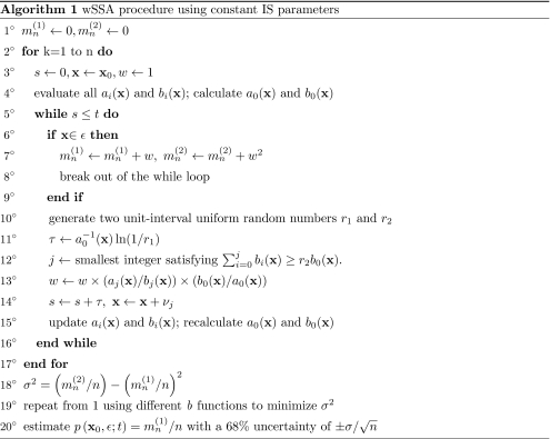
The current algorithm can be seen in Fig. 1.

Figure 1.

The weighted stochastic simulation algorithm using constant importance sampling parameters.

THE STATE-DEPENDENT BIASING METHOD

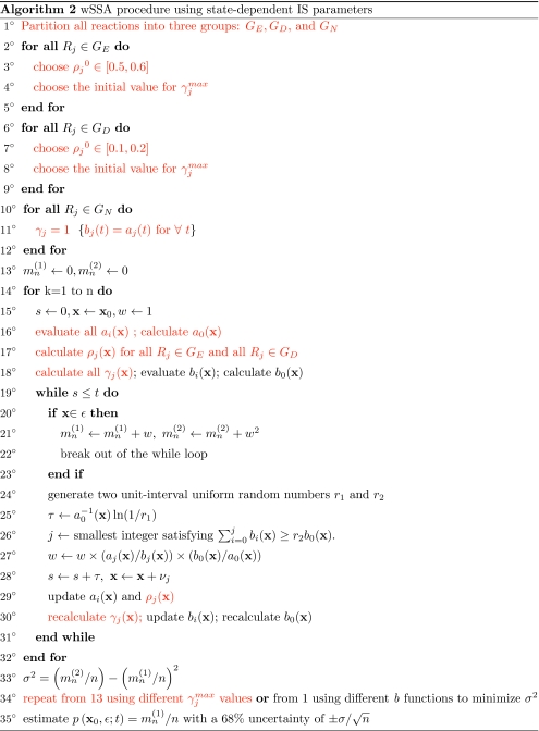
The key element of the wSSA is importance sampling, which is a general technique often used with a Monte Carlo method to reduce the variance of an estimate of interest. The rationale for using this technique is that not all regions of the sample space have the same importance in simulation. When we have some knowledge about which sampling values are more important than others, we can use important sampling to improve efficiency as well as accuracy. The technique involves choosing an alternative distribution from which to sample the random numbers. This alternative distribution is chosen such that the important samples are chosen more frequently than they are in the original distribution. After using the alternative distribution to sample, a correction is applied to ensure that the new estimate is unbiased. The wSSA employs this technique in the reaction selection procedure. The next reaction is chosen using b(x) (12° in Algorithm 1), and the bias is corrected with an appropriate weight, (a_j(x)∕b_j(x))×(b₀(x)∕a₀(x)) (13°). Mathematical details of importance sampling and Monte Carlo averaging can be found in Appendix of Ref. 2.

The current method for selecting b functions is to simply multiply the original propensities by a positive scalar γ_j, i.e., b_j(x)=γ_ja_j(x). The fixed multiplier facilitates the wSSA implementation, but there are several associated drawbacks. The most obvious drawback is increased variance due to over- and underperturbations. The changes in species population during the simulation cause the relative propensity of reaction j, a_j(x)∕a₀(x), to fluctuate as well, changing the probability of selecting the jth reaction at each time step. If γ_j is constrained to be a constant for all possible values of a_j(x)∕a₀(x), then the optimal value for γ_j would be the one that perturbed a_j “just right” for most values of a_j(x). However, if a_j(x)∕a₀(x) varied widely, then γ_j would over- or underperturb a_j(x) near the extreme values of a_j(x)∕a₀(x). A related drawback concerns a narrow parameter space of γ_j that produces an accurate estimate for p(x₀,ε;t). If a_j(x)∕a₀(x) reaches values near 0 as well as 1 during a single simulation, then it is impossible to avoid both over- and underperturbations because the jth importance sampling parameter can have only a single value which can avoid only one of the two cases. Thus, there will be very few values for γ_j that produce an accurate estimate. Unless the initial value for γ_j is set near these few values, the resulting estimate is guaranteed to have high variance. This unreliable estimate is not useful in deciding how to perturb γ_j to obtain an estimate with lower variance (step 19° of the Algorithm 1). Consequently, one may waste a lot of computational power searching for a value of γ_j that produces an accurate estimate.

Since the above problems are due to fluctuations in the propensity, which is caused by fluctuations in population size, an intuitive solution would be to vary γ_j according to the current state x. Although an arbitrary function may be used to achieve such goal, we proceed as follows.

First, we partition reactions into three groups:G_E, G_D, and G_N. We define G_E as the set of reactions that are to be encouraged. This set may include reactions that directly or indirectly increase the likelihood of rare event observation. The IS parameters for this group have values greater than 1 to increase the reaction firing frequency. Similarly we define G_D as the set of reactions that are to be discouraged. The IS parameters for G_D will be between 0 and 1, to decrease the likelihood of firing a reaction in G_D. All reactions that do not influence the rare event observation are grouped into G_N. Since the reactions in G_N do not need to be perturbed, the IS parameters for these reactions are set to 1. We note that in practice, optimal partitioning of the reactions requires knowledge of the system, which may not always be available.

Second, we define the relative propensity of reaction j as ρ_j(x)≡a_j(x)∕a₀(x). ρ_j(x) is a fractional propensity between 0 and 1 that roughly indicates the likelihood of choosing R_j as the next reaction from the current state x. Since the value of ρ_j at each time step gives a qualitative indication of the amount of perturbation needed by R_j, the new biasing method will define γ_j to be a function of ρ_j.

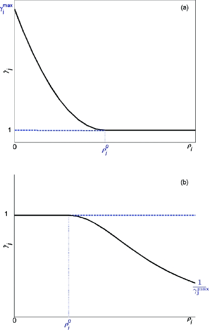
When ρ_j→0, the probability of choosing R_j as the next reaction decreases. Thus, for R_j∊G_E, more encouragement is needed as its relative propensity decreases. However, when ρ_j≈1, R_j is likely to be selected as the next reaction without any additional encouragement. In this case, taking b_j(x)>a_j(x) will overperturb the system and thus increase the variance in the estimate. Therefore, for R_j∊G_E, there must be a value of ρ_j at which no further encouragement is applied. Similarly for R_j∊G_D, no further discouragement is necessary when ρ_j≈0. The value of ρ_j for which we stop the perturbation is defined as ρ_j⁰, i.e., γ_j=1 for ρ_j≥ρ_j⁰(R_j∊G_E) and for ρ_j≤ρ_j⁰(R_j∊G_D). Lastly for R_j∊G_D, more discouragement is necessary as ρ_j increases. This corresponds to γ_j→0 as ρ_j→1.

Based on above considerations, we take the jth IS parameter of R_j∊G_E as

$${\gamma }_j\left({\rho }_j\left(\mathbf{x}\right)\right)=\{\begin{array}{ll}1\hfill & \text{if}{\rho }_j\left(\mathbf{x}\right)\ge \rho _j{}^0,\hfill \\ g_j\left({\rho }_j\left(\mathbf{x}\right)\right)\hfill & \text{if}{\rho }_j\left(\mathbf{x}\right)<\rho _j{}^0\hfill \end{array}\phantom{\}}$$ (8)

where g_j(ρ_j) is a parabolic function of ρ_j that has the following properties:

$$g_j\left(0\right)={\gamma }_j^{\text{max}},$$$$g_j\left(\rho _j{}^0\right)=1,$$$$g_j^{\prime }\left(\rho _j{}^0\right)=0.$$ (9)

For R_j∊G_D, we select γ_j as the following:

$${\gamma }_j\left({\rho }_j\left(\mathbf{x}\right)\right)=\{\begin{array}{cc}1& \text{if}{\rho }_j\left(\mathbf{x}\right)\le \rho _j{}^0\\ \frac{1}{h_j\left({\rho }_j\left(\mathbf{x}\right)\right)}& \text{if}{\rho }_j\left(\mathbf{x}\right)>\rho _j{}^0,\end{array}\phantom{\}}$$ (10)

where h_j(ρ_j) is a parabolic function of ρ_j that has the following properties:

$$h_j\left(1\right)={\gamma }_j^{\text{max}},$$$$h_j\left(\rho _j{}^0\right)=1,$$$$h_j^{\prime }\left(\rho _j{}^0\right)=0.$$ (11)

Graphical representations of the function γ_j(ρ_j(x)) are illustrated in Fig. 2, for R_j∊G_E and R_j∊G_D.

Figure 2.

(a) A graphical representation of γ_j(ρ_j(x)) for R_j∊G_E. (b) A graphical representation of γ_j(ρ_j(x)) for R_j∊G_D.

There are two parameters, ${\gamma }_j^{\text{max}}$ and ρ_j⁰, for each γ_j(ρ_j(x)). ${\gamma }_j^{\text{max}}$ is defined as the parameter associated with the maximum perturbation allowed on the jth reaction. Given the values for ${\gamma }_j^{\text{max}}$ and ρ_j⁰, g_j(ρ_j), and h_j(ρ_j) as defined in Eqs. 9, 11 are unique parabolas whose formula is

$$g_j\left({\rho }_j\right)=\left(\frac{{\gamma }_j^{\text{max}}-1}{{\left(\rho _j{}^0\right)}^2}\right){\left(\rho _j{}^0-{\rho }_j\right)}^2+1\left(\text{if}{R}_j∊G_E\right),$$$$h_j\left({\rho }_j\right)=\left(\frac{{\gamma }_j^{\text{max}}-1}{{\left(\rho _j{}^0-1\right)}^2}\right){\left(\rho _j{}^0-{\rho }_j\right)}^2+1\left(\text{if}{R}_j∊G_D\right).$$ (12)

An important point to keep in mind is that perturbing a_j(x) by an unnecessarily large amount not only potentially increases the number of rare event observations but also increases the variance of an estimate as well. We want to observe enough rare events to calculate necessary statistics, yet at the same time to minimize the variance. The advantage of using γ_j(ρ_j) is that a user has the freedom to choose ${\gamma }_j^{\text{max}}$ and ρ_j⁰, whose optimal values are problem dependent. Currently, there is no fully automated method to find the optimal value for the two parameters. For the examples in Sec. 4, we first choose a value for ρ_j⁰ by assigning a value near 0.15±0.05 (R_j∊G_D) or 0.55±0.05 (R_j∊G_E). We then vary ${\gamma }_j^{\text{max}}$ to find an estimate with the lowest parameter.

After incorporating the new strategy for choosing γ_j, we obtain the algorithm in Fig. 3.

Figure 3.

The weighted stochastic simulation algorithm using state-dependent importance sampling parameters. Changes from Fig. 1 are highlighted in red.

NUMERICAL EXAMPLES

In this section we illustrate our new biasing algorithm with three examples, comparing the results with those obtained using the original algorithm. As we will see, the new biasing method increases the computational speed not only relative to the SSA but also relative to the scheme used in the original wSSA papers.^{1, 2} The measure used to calculate gain in computational efficiency is the same as in Ref. 2, given by

$$g\equiv \frac{n^{\text{SSA}}}{n^{\text{wSSA}}},$$ (13)

where n^SSA and n^wSSA are the numbers of runs in each of the two methods required to achieve comparable accuracy.

Two-state conformational transition

Consider the following system:

$$A\underset{k_2}{\overset{k_1}{\rightleftarrows }}B,\text{with}{k}_1=0.12\text{and}{k}_2=1.$$ (14)

The initial state is set to x₀=[100 0], i.e., all 100 molecules are initially in A form. This model concerns two conformational isomers—isomers that can be interconverted by rotation about single bonds. For this system we are interested in p(0,30;10) for B; that is, the probability that given no B molecules at time 0, its population reaches 30 before time 10. The steady-state population of B for the rate constants in Eq. 14 is approximately 11. The rare event description of x₂=30 is about three times its steady-state value, so we expect its probability to be very small. Because this is a simple closed system, it is possible to calculate the exact probability of p(0,30;10) using a generator matrix (or a probability transition matrix).⁴ Using MATLAB’s matrix exponential function, we have calculated p(0,30;10)=1.191×10⁻⁵.

Since the steady-state population of B is much less than the rare event description of 30, it is necessary to bias the system so that the population of B increases. This can be achieved by either encouraging R₁ or discouraging R₂. Note that changing the propensities of both reactions is not necessary, as only the relative ratio of the two propensities matters in reaction selection.

For simulation of system 14 with the original wSSA, R₁ was encouraged with different values of γ₁>1. Thus, the b functions are given by

$$b_1\left(\mathbf{x}\right)={\gamma }_1{a}_1\left(\mathbf{x}\right),b_2\left(\mathbf{x}\right)=a_2\left(\mathbf{x}\right).$$ (15)

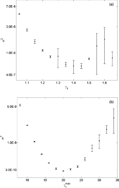
To find the γ₁ that produces the minimum variance, γ₁ was varied from 1.05 to 1.65 in increments of 0.05. Of these values, γ₁=1.4 produced the lowest variance. Taking n=10⁷ and γ₁=1.4, the following estimate±twice the uncertainty (95% confidence interval) was obtained:

$$p\left(0,30;10\right)=1.21\times {10}^{-5}\pm 0.06\times {10}^{-5}.$$ (16)

In the new biasing method, we replicated the reaction partition as done in the original system, i.e., G_E={R₁}, G_D={∅}, G_N={R₂}. After assigning ρ₁⁰=0.5, ${\gamma }_1^{\text{max}}$ was varied from 8 to 34 in increments of 2. Using n=10⁵ and the optimal ${\gamma }_1^{\text{max}}=20$, the following estimate was obtained with a 95% confidence interval:

$$p\left(0,30;10\right)=1.190\times {10}^{-5}\pm 0.011\times {10}^{-5}.$$ (17)

Although both estimates contain the true probability in their 95% confidence interval, the new biasing method required only 1% of the total number of simulations used in the original algorithm. Furthermore, the new biasing method produced a more accurate estimate with a much tighter confidence interval. Figure 4 shows a side by side comparison of σ² for p(x₀,30;10) using both biasing methods. We note that the new algorithm not only decreased the variance by a factor of 1000 but also produced an accurate estimate with a larger range of ${\gamma }_1^{\text{max}}$. Given n=10⁷, the previous algorithm was able to produce an accurate estimate with a narrow range of γ₁∊[1.10 1.60]. In contrast, any estimate from using the new biasing method with ${\gamma }_1^{\text{max}}∊\left[834\right]$ produced more accurate estimate than Eq. 16.

Figure 4.

(a). A plot of σ² vs γ₁ obtained in wSSA runs of reaction Eq. 14 using the algorithm in Fig. 1. Here we estimate p(0,30;10) for B. Each vertical bar shows the estimated mean and one standard deviation of σ² at that γ₁ value as found in four n=10⁷ runs. (b) A plot of σ² vs ${\gamma }_1^{\text{max}}$ obtained from using the algorithm in Fig. 3. Each vertical bar was obtained from four n=10⁵ runs.

Using the SSA to obtain an estimate with similar variance as in Eq. 17 would require a much greater computational expense. For our particular simulation, the calculated efficiency gain of the new algorithm over the SSA was 4.1×10⁴, i.e., it would have taken a computer 4.1×10⁴ times longer to obtain a similar result using the unweighted SSA.

Single species production and degradation

Our next example is taken from Refs. ^{1, 2} and consists of the following two reactions:

$$S_1\stackrel{k_1}{\to }{S}_1+S_2,S_2\stackrel{k_2}{\to }\varnothing \text{with}{k}_1=1\text{and}{k}_2=\mathrm{0.025.}$$ (18)

The initial state of the system is x₀=[1 40], and we are interested in p(40,80;100) for S₂—the probability that x₂ reaches 80 before time 100 given x₂=40 at t=0. This particular reaction set is well-studied, and it is known that the population of S₂ in its steady-state follows the Poisson distribution with mean (and variance) of k₁x₁∕k₂. Since the initial state of S₂ is also its steady-state mean, x₂ is expected to fluctuate around 40 with a standard deviation of 6.3. To advance the system toward the rare event, R₁ was chosen to be encouraged in both of the following wSSA simulations.

First, 4×10⁷ wSSA simulations were performed for each γ₁ ranging from 1.45 to 2.25 in increment of 0.05. The following estimate was obtained using the optimal γ₁=1.85:

$$\begin{array}{c}p\left(40,80;100\right)=2.985\times {10}^{-7}\pm 0.020\times {10}^{-7}\\ \left(95\mathrm{\%}\text{confidence}\right).\end{array}$$ (19)

We repeated the simulation with the new state-dependent biasing method which encouraged R₁ as was done with the original algorithm. After running only 10⁵ simulations with ρ₁⁰=0.6 and different values of ${\gamma }_1^{\text{max}}$, we obtained the following result using the optimal ${\gamma }_1^{\text{max}}=14$:

$$\begin{array}{c}p\left(40,80;100\right)=2.986\times {10}^{-7}\pm 0.019\times {10}^{-7}\\ \left(95\mathrm{\%}\text{confidence}.\right)\end{array}$$ (20)

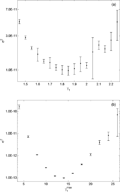
Figure 5 shows a side by side comparison of the variance using both biasing methods. As is shown, the biasing method with a state-dependent importance sampling parameter yielded estimates with variance two orders of magnitude less than that produced using the constant parameter importance sampling parameter. We also note that the latter simulation required 100 times fewer simulations to obtain a result with equivalent accuracy and uncertainty 20, which is a significant improvement over Eq. 19. Furthermore, the variance of an estimate generated by using any ${\gamma }_1^{\text{max}}∊\left(4,26\right)$ is lowerthan the variance of estimate 19. Lastly, the computational efficiency gain of Eq. 20 over SSA was 3.1×10⁶, which is more than 100 times the gain from using the original biasing method.

Figure 5.

(a) A plot of σ² vs γ₁ obtained in wSSA runs of reaction 18 using the algorithm in Fig. 1. Here we estimate p(40,80;100) for S₂. Each vertical bar shows the estimated mean and one standard deviation of σ² at that γ₁ value as found in four n=4×10⁷ runs. (b) A plot of σ² vs ${\gamma }_1^{\text{max}}$ obtained from using the algorithm in Fig. 3. Each vertical bar was obtained from four n=10⁵ runs.

Modified yeast polarization

Our last example concerns pheromone induced G-protein cycle in Saccharomyces cerevisia⁵ with a constant population of ligand, L=2. The model description was modified from Ref. 5, such that the system does not reach equilibrium. There are six species in this model, x=[RGRLG_aG_bgG_d] and eight reactions as follows:

$$\text{R}1:\varnothing \stackrel{k_{R_s}}{\to }R,$$$$\text{R}2:R\stackrel{k_{R_d}}{\to }\varnothing ,$$$$\text{R}3:L+R\stackrel{k_{RLL}}{\to }RL+L,$$$$\text{R}4:RL\stackrel{k_R}{\to }R,$$$$\text{R}5:RL+G\stackrel{k_{G_a}}{\to }{G}_a+G_{bg},$$$$\text{R}6:G_a\stackrel{k_{G_d}}{\to }{G}_d,$$$$\text{R}7:G_d+G_{bg}\stackrel{k_G}{\to }G,$$$$\text{R}8:\varnothing \stackrel{k_{RL}}{\to }RL.$$ (21)

The kinetic parameters are

$$k_{R_s}=0.0038,k_{R_d}=4.00e-4,k_{RLL}=0.042,$$

$$k_R=0.0100,k_{G_a}=0.011,k_{G_d}=0.100,$$

$$k_G=1.05e+3,k_{RL}=\mathrm{3.21.}$$

The state representing the initial condition is x₀=[50 50 0 0 0 0]—there are 50 molecules of R and G, but none of the other species are initially present. For this system, we define the rare event to be p(x₀,ε_Gbg;20), where ε_Gbg is the set of all states x for which the population of G_bg is equal to 50. We first partition the reactions as G_E={∅}, G_D={R₆}, and G_N={R₁,..,R₅,R₇,R₈}. The only reaction chosen to be perturbed is R₆, which indirectly discourages the consumption of G_bg by delaying the production of G_d. Here we note that a more intuitive choice of reactions to include in G_D would be R₇, since it directly consumes a G_bg molecule. Upon numerical testing, however, we found that the estimate from perturbing R₇ showed much higher variance than the one obtained from discouraging R₆. This difference in performance is due to the four orders of magnitude separating the reaction constants k_Gd and k_G. Because the reaction constant k_G is so large, an extremely small IS parameter is required to effectively discourage R₇. The results from our testing indicate that such a small IS parameter confers high variance. In contrast, the IS parameter needed by R₆ was more modest and led to much better performance.

Following the partitioning with G_D={R₆}, the b functions for the constant parameter biasing method are

$$b_6=\frac{1}{{\gamma }_6}{a}_6,$$$$b_j=a_j,\text{j}=1,2,3,4,5,7,8.$$ (22)

First, we ran 10⁸ simulations of wSSA for each of the constant IS parameter γ₆, where γ₆ ranged from 1.2 to 2.0 in increments of 0.1. Then 10⁸ simulations with the state-dependent biasing method was conducted for each ${\gamma }_6^{\text{max}}=\left\{12,14,\dots ,22,24\right\}$ with ρ₆⁰=0.15, where the b functions are given by

$$b_6={\gamma }_6\left({\rho }_6\right)a_6,$$$$b_j=a_j,\text{j}=1,2,3,4,5,7,8.$$ (23)

Because R₆∊G_D, the value of γ₆ at each time step is chosen according to h_j(ρ_j) in Eq. 12. The best IS parameter, γ=1.5, from the first set of simulations yields the following estimate:

$$\begin{array}{c}p\left({\mathbf{x}}_0,{\epsilon }_{G_{bg}};20\right)=1.23\times {10}^{-6}\pm 0.05\times {10}^{-6}\\ \left(95\mathrm{\%}\text{confidence}\right).\end{array}$$ (24)

The best estimate from using the state-dependent IS method with γ^max=3 yields

$$\begin{array}{c}p\left({\mathbf{x}}_0,{\epsilon }_{G_{bg}};20\right)=1.202\times {10}^{-6}\pm 0.014\times {10}^{-6}\\ \left(95\mathrm{\%}\text{confidence}\right).\end{array}$$ (25)

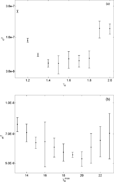
System 21 exhibits high intrinsic stochasticity, which causes difficulty in obtaining an estimate with low variance unless a large n is used. Despite this difficulty, we see that the uncertainty of the estimate obtained from using the state-dependent biasing algorithm is about three times less than the uncertainty in Eq. 24. Figure 6 shows a side by side comparison of σ² for p(x₀,ε_Gbg;20), and we see that the variance in Fig. 6b is less than the variance in Fig. 6a by a factor of 10. In addition to increased accuracy, the new method also provides increased robustness, in that it provides a broader range of acceptable values for its parameter ${\gamma }_6^{\text{max}}\left(12–24\right)$ than for the old method’s parameter γ₆(1.3–1.8).

Figure 6.

(a) A plot of σ² vs γ₆ obtained in wSSA runs of reaction 21 using the algorithm in Fig. 1. Here we estimate p(0,ε_Gbg;20), where ε_Gbg is the set of all states x in which the population of G_bg is 50. Each vertical bar shows the estimated mean and one standard deviation of σ² at that γ₆ value as found in four n=10⁸ runs. (b) A plot of σ² vs ${\gamma }_6^{\text{max}}$ obtained from using the algorithm in Fig. 3. Each vertical bar was obtained from four n=10⁸ runs.

The computational gain of wSSA from using a constant importance sampling parameter is 21, while that of the state-dependent importance sampling method is 250. Both gains imply a significant speed up against the SSA considering that the simulation time for 10⁸ wSSA trajectories of system 21 is several days.

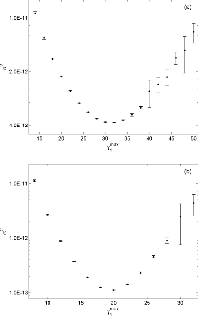
Lastly, we comment that although the value of ρ_j⁰ is chosen arbitrarily from a specified range (0.15±0.05 for R_j∊G_D and 0.55±0.05 for R_j∊G_E), the performance of the state-dependent biasing algorithm remains almost the same for different values of ρ_j⁰. For R_j∊G_E, the lower and upper boundary values for ρ_j⁰ are 0.5 and 0.6, respectively. Figure 5b of system 18 was obtained using ρ₁⁰=0.6, which is the upper boundary value of ρ_j⁰ range. To compare the performance of the new algorithm for system 18 using different values of ρ₁⁰, we have created a plot of variance versus ${\gamma }_1^{\text{max}}$ with two different values of ρ₁⁰∊{0.5,0.55}, which are lower boundary and median value [Figs. 7a, 7b]. We see that the minimum variance from both subplots of Fig. 7 is of similar magnitude compared to the minimum variance in Fig. 5b. Similar observation can be made for the other two examples.

Figure 7.

(a) A plot of σ² vs ${\gamma }_1^{\text{max}}$ obtained in wSSA runs of reaction 18 using ${\rho }_1^0=\mathrm{0.5.}$ Here we estimate p(40,80;100) for S₂. Each vertical bar shows the estimated mean and one standard deviation of σ² at that ${\gamma }_1^{\text{max}}$ value as found in four n=10⁵ runs. (b) A plot of σ² vs ${\gamma }_1^{\text{max}}$ obtained using the same setting as in Fig. 7a, except ρ₁⁰=0.55.

CONCLUSIONS

In this paper we have introduced a state-dependent biasing method for the weighted stochastic simulation algorithm. As numerical results from Sec. 4 support, the new state-dependent biasing method improves the accuracy of a rare event probability estimate and speeds up the simulation time. While the state-dependent biasing method excels in many aspects, it involves twice the number of parameters than the constant parameter biasing method. Currently, there is no automated method to assign an appropriate value to these parameters, and thus the computational effort associated with this task can be challenging as system size increases. It may be thought that using a line instead of a parabola in Eq. 12 would simplify the algorithm. However, owing probably to the nonlinearity of propensities that involve more than one species, we have found that the parabola usually works better. We have also observed in our numerical experiments that using a line has a negative impact on robustness, as compared to a parabola.

As noted in Sec. 3, the new biasing algorithm toggles between the original propensities and the biased propensities to select the next reaction, depending on the value of ρ_j(x). Therefore, the wSSA using the state-dependent biasing method can be regarded as an efficient adaptive algorithm. However, the value for two parameters ρ_j⁰ and ${\gamma }_j^{\text{max}}$ must be determined prior to the simulation, and correctly partitioning reactions into three groups (G_E, G_D, and G_N) can be challenging for large systems. These issues will be explored in future work.

References

- Kuwahara H. and Mura I., J. Chem. Phys. 129, 165101 (2008). 10.1063/1.2987701 [DOI] [PubMed] [Google Scholar]
- Gillespie D. T., Roh M., and Petzold L. R., J. Chem. Phys. 130, 174103 (2009). 10.1063/1.3116791 [DOI] [PMC free article] [PubMed] [Google Scholar]
- Chan T. F., Golub G. H., and Leveque R. J., Am. Stat. 37, 242 (1983). 10.2307/2683386 [DOI] [Google Scholar]
- Nelson R., Probability, Stochastic Processes, and Queuing Theory: The Mathematics of Computer Performance Modeling (Springer, New York, 1995). [Google Scholar]
- Drawert B., Lawson M. J., Petzold L. R., and Khammash M., J. Chem. Phys. 132, 074101 (2010). 10.1063/1.3310809 [DOI] [PMC free article] [PubMed] [Google Scholar]