Systems Biology—Biomedical Modeling

Abstract

Because of the complexity inherent in biological systems, many researchers frequently rely on a combination of global analysis and computational approaches to gain insight into both (i) how interacting components can produce complex system behaviors, and (ii) how changes in conditions may alter these behaviors. Because the biological details of a particular system are generally not taught along with the quantitative approaches that enable hypothesis generation and analysis of the system, we developed a course at Mount Sinai School of Medicine that introduces first-year graduate students to these computational principles and approaches. We anticipate that such approaches will apply throughout the biomedical sciences and that courses such as the one described here will become a core requirement of many graduate programs in the biological and biomedical sciences.

The Need for a Systems Biology Course

Systems biology focuses on developing an understanding of how phenotypic behavior of the system as a whole emerges from the components and interactions that constitute the system. Systems studied may be at various scales; they can be at the subcellular, cellular, tissue or organ, or organismal level. Regardless of the scale, a key feature of systems biology is that properties of and interactions among many components are studied, rather than simply the characteristics of individual molecules. This course focuses mainly on the analysis of systems at the subcellular and cellular level, although similar principles apply when other scales are analyzed.

Advances in biological sciences over the past several decades have made it clear that most biological systems are extremely complex. This inherent complexity makes it difficult, if not impossible, to understand emergent behaviors, such as cellular decisions and phenotypes, using only intuition. Systems biology, therefore, relies on a combination of experiments that measure multiple entities simultaneously and computational approaches that allow the analysis of multivariate data and the generation of testable predictions. Experimental techniques that are critical to systems biology are frequently taught in undergraduate and graduate programs in biomedical sciences. Computational approaches, however, have traditionally not been part of these curricula. We describe a course developed at Mount Sinai School of Medicine that introduces first-year graduate students to computational techniques applicable to systems biology and that uses relevant biological examples, with the implicit assumption that such approaches will become increasingly important, not just in systems biology (1), but in the biomedical sciences more generally.

Computational Needs of Systems Biology

Systems biology uses a range of computational techniques to analyze data sets of varying sizes and types and to build predictive models. Although these computational methods are used individually in other biological and physical sciences, a distinct combination is often employed in systems biology research (Fig. 1).

Fig. 1.

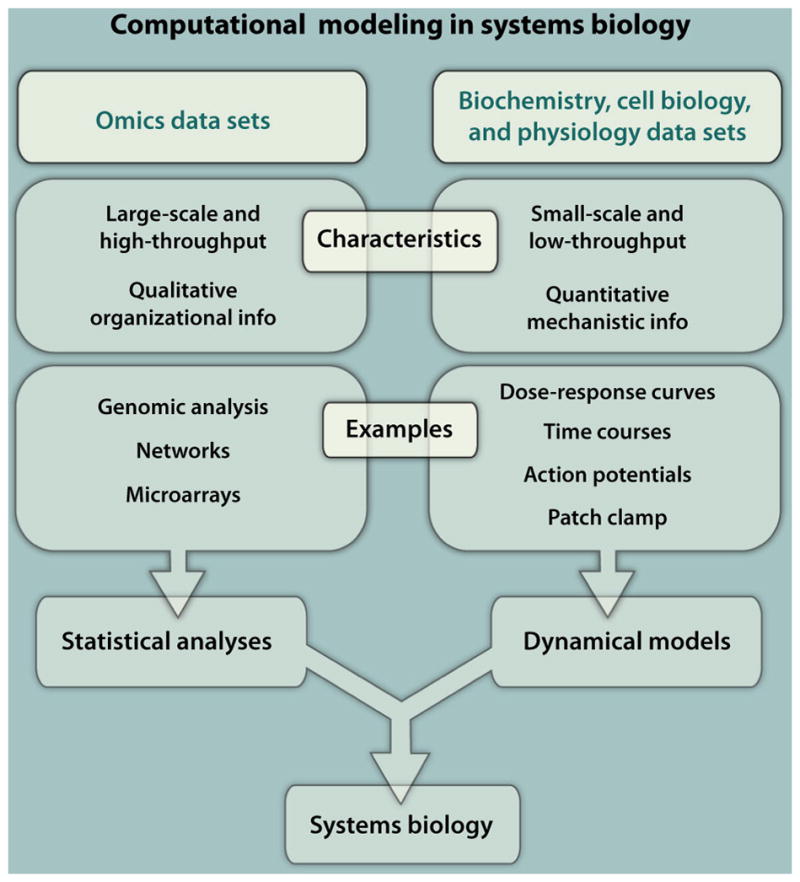
Data sets can dictate the computational approaches used in systems biology. (Left) Omics technologies generate extremely large data sets that can be analyzed and organized into networks by using statistical modeling techniques. This strategy can be considered “top-down” modeling. (Right) When high-quality data are available, smaller-scale systems can be represented by dynamical models, and simulations with these models can generate quantitative predictions of system behavior. This strategy is sometimes called “bottom-up” modeling. Both approaches are important in systems biology, and a few cutting-edge studies combine the positive aspects of both.

In general, two major experimental approaches are used in systems biology, yielding different types and volumes of data. One approach involves the gathering of large data sets, often through high-throughput assays, and subsequent analyses of these data sets (Fig. 1, left). In these types of experiments, the researchers obtain a vast and sometimes comprehensive picture of the changes that occur in response to a defined perturbation, such as the induction of a disease state. These large-scale and frequently genome-, proteome-, or metabolome- wide studies are often referred to as “omic” data sets. For instance, the measurement of changes in abundance of thousands of mRNAs by microarray (2) or next-generation sequencing (3) is now a fairly routine experimental procedure. Other examples of large data sets include analyses of the whole genome for transcription factor–binding sites and epigenetic markings; proteomic data sets that measure changes of protein abundance or posttranslational modifications, such as phosphorylation; and metabolomics that measure changes in composition and concentrations of metabolites. Omic data sets can be so vast that sophisticated computational algorithms are required to even visualize and gain a qualitative appreciation of the results. Thus, statistical and network modeling approaches are critical for analyzing data obtained with high-throughput assays. These modeling techniques can render the data amenable to human investigation and discovery, revealing patterns in the data, which can help to determine the pathways and processes involved. This level of analysis provides insight into the organization of and relations among the components and can generate predictions of how the system will respond to a perturbation, such as knockout of a gene.

The second approach involves the study of fewer components, but in greater depth so as to understand the quantitative relation between the components and the emergent behaviors that arise from these interactions (Fig. 1, right) (4). Experiments generally measure key system variables as a function of time and sometimes also as a function of space. Time courses may be recorded in response to multiple perturbations, and data may be summarized as dose-response curves. These systems are analyzed using dynamical models that can simulate the time evolution of the system’s behavior. When representations of average behavior are adequate, the dynamical models are generally deterministic (4). This means that a particular set of parameters and initial conditions will always generate the same output. If fluctuations of individual molecules need to be considered, then stochastic models that incorporate randomness may be used (5). Both types of dynamical models can generate quantitative predictions that can subsequently be tested experimentally. From this iteration between simulation and experiment, mechanisms of regulation that are operative at a systems level, such as feedback and feed-forward loops (6) can be inferred (Fig. 2). Thus, the questions addressed by dynamical models focus on mechanisms that give rise to emergent properties at a systems level.

Fig. 2.

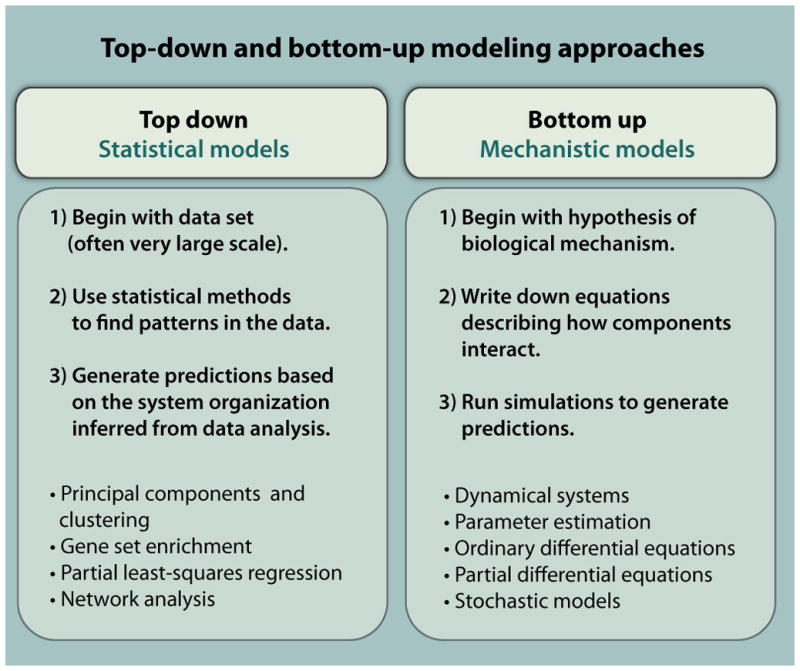
Complementary computational approaches used in systems biology. For either the top-down approach (left) or the bottom-up approach (right), the text describes the general strategy of computational studies (middle) and lists important techniques that are taught in the course.

Several studies that have combined experiments with computation have operated at what might be considered an intermediate level (mesoscale) of complexity (7, 8). These studies have measured the activities of tens, rather than hundreds or thousands, of signaling molecules. Although the data obtained in these studies were not sufficiently detailed, in terms of rates or concentrations, to enable construction of dynamical models, the work showed that relatively straightforward input-output relations generated through methods such as regression had impressive predictive power (7, 8). Thus, the modeling approach that is suited to a given study depends to a large extent on the nature of the data and the depth of understanding of the system under consideration.

The course is organized to provide students with a well-rounded knowledge of the full range of computational techniques used in cutting-edge studies, while emphasizing the appropriate computational technique for a particular set of data. The course introduces students to both statistical and network modeling techniques that are particularly important for analyzing omics data sets and to dynamical modeling techniques that provide quantitative mechanistic insight into data obtained in cell biology and physiology experiments. This combination of computational approaches leads to the identification of the topology and organizational characteristics of the system through the application of statistical and network models, and then an understanding of the regulatory and functional capabilities of the system through the application of dynamical models.

Student Prerequisites

The course is designed for students who have taken upper-level undergraduate courses in cell and molecular biology. Students should have a basic knowledge of statistics; however, no prior programming or modeling experience is necessary.

Course Organization and Topics

The course is designed as a 3-credit course with three teacher-student contact hours per week for a 15-week semester and includes ~ 3 to 5 hours per week of homework assignments (Table 1). There are 12 Teaching Resources published in sequential issues of Science Signaling that provide lecture notes, slides, problem sets, and answer keys (Table 1). The topics covered and a brief summary of the Teaching Resources are provided here.

Table 1.

Course schedule and Teaching Resources for the Systems Biology course.

Teaching Resource	Lecture Number	Lecture Topic
None	1	Overview of course—Introduction to modeling
Introduction to Statistical Methods to Analyze Large Data Sets: Principal Components Analysis	2	Trends in large data sets: Principal components analysis
Introduction to Statistical Methods for Analyzing Large Data Sets: Gene Set Enrichment Analysis	3	Analysis of large data sets: Gene set enrichment analysis
Introduction to Network Analysis in Systems Biology	4	Representation of biological systems as networks
	5	Milestones and key concepts in network analysis
	6	Making predictions using network analysis
None	7	Discussion and problem-solving session
An Introduction to Dynamical Systems	8	Introduction to dynamical systems
Introduction to MATLAB	9	Computing with MATLAB I
	10	Computing with MATLAB II
Obtaining and Estimating Kinetic Parameters from the Literature	11	Development of models I: Extracting constants from experimental literature and estimating errors
Biomedical Model Fitting and Error Analysis	12	Development of models II: Curve fitting and error estimation
None	13	Discussion and problem-solving session
Bistability in Biochemical Signaling Models	14	Ordinary differential equation models of bistability in biochemical signaling I
	15	Ordinary differential equation models of bistability in biochemical signaling Ii
Computational Modeling of the Cell Cycle	16	Ordinary differential equation model of the cell cycle
None	17	Ordinary differential equation model of the action potential
None	18	Discussion and problem-solving session
None	19	Partial differential equation model of a propagating action potential
Developing Models in Virtual Cell	20	Spatial models in virtual cell: Ordinary differential equations and partial differential equations
None	21	Discussion and problem-solving session
Probabilistic Reasoning in Data Analysis	22	Analysis of data from stochastic events
Simulations of Stochastic Biological Phenomena	23	Stochastic models I
	24	Stochastic models II
None	25	Discussion and problem-solving session

The beginning of the course focuses on statistical approaches and network modeling. The first two Teaching Resources cover lectures 2 and 3, which introduce methods used to analyze large data sets. The first introduces principal component analysis (PCA) as an approach for identifying trends within large data sets and reducing data dimensionality for visualization. The second Teaching Resource introduces the students to gene set enrichment analysis (GSEA), which combines statistical methods with prior knowledge about the biological system. The third Teaching Resource describes lectures 4, 5, and 6, which deal with graph theory and network analyses. The students are introduced to key concepts in graph theory and how networks can be built from either large experimental data sets or from data in the biochemical and cell biological literature. Methods to analyze both global and local characteristics of networks are presented. These include topological analyses to identify network motifs, such as feedback loops, feed-forward motifs, and bifan motifs. Methods for network visualization and identification of functional units within cellular networks are also presented.

Another main topic of the course is an introduction to dynamical models, which are used to obtain quantitative input and output relations with respect to time and space. Deterministic dynamical models, which use ordinary or partial differential equations as the mathematical basis for the model, are fully specified by the equations and the initial conditions of the system. Stochastic models incorporate the effects of randomness, and repeated simulations can therefore generate different results. Exploiting the power of dynamical models requires knowing several important concepts that are discussed in turn during the course. Because MATLAB is the software package used in the course for the implementation and analysis of dynamical models, a Teaching Resource that describes two lectures introducing this software (lectures 9 and 10) is included. The Teaching Resource corresponding to lecture 8 illustrates how to analyze ordinary differential equation (ODE) models using the tools of dynamical systems theory. These concepts are further elaborated in a Teaching Resource associated with lectures 14 and 15, which describe switching behavior or bistability, and a Teaching Resource associated with lecture 16, which covers mathematical models of the cell cycle.

ODE models of biological processes require the user to specify reaction rates and the initial concentrations of reactants. For many biochemical reactions, these numbers are not available; therefore, they have to be estimated from experiments conducted for other purposes. The Teaching Resource associated with lecture 11 presents methods for estimating kinetic parameters and concentrations of cellular components. All numerical simulations have some errors associated with the computation. These errors need to be explicitly estimated and taken into consideration during the interpretation of the results of the simulations. Therefore, the next Teaching Resource associated with lecture 12 presents methods for error estimation.

Virtual Cell, developed by a group at the University of Connecticut (9), is a tool for developing cellular models that incorporate spatial organization. Therefore, the Teaching Resource associated with lecture 20 introduces students to this modeling platform, which allows the user to import realistic microscopic images, including images from live cell experiments. Models built with this platform can simulate complex cellular phenomena, such as cyclic adeno sine monophosphate microdomains, calcium waves, and nuclear-cytoplasmic transport.

The final topic covered in the course is the use of probabilistic models for analysis of stochastic systems. Several biological processes are probabilistic in nature, where-by a system variable, such as the concentration of a protein or a second messenger or an ion, may exhibit large fluctuations. For instance, single-cell measurements have shown that the behavior of individual cells can deviate considerably from the average behavior of the group. Methods for modeling such stochastic processes are an important aspect of quantitative biology, and the last set of Teaching Resources therefore describes lectures on stochastic modeling. Lecture 22 and the associated Teaching Resource introduce probabilistic thinking and show through classic examples how a rigorous analysis of data can lead to deep understanding of underlying biological phenomena. Lectures 23 and 24 and the associated Teaching Resource describe methods for simulating stochastic phenomena by applying the classic Gillespie algorithm to a model of transcription and translation.

Course Goals and Outcomes

The overall goal of this course is to train the students in the range of computational approaches that are used in systems biology. These include (i) analysis of large data sets, (ii) development and analysis of networks, (iii) application of deterministic dynamical models consisting of ordinary or partial differential equations, and (iv) application of stochastic dynamical models.

This is a laboratory course in which the students perform numerical computations during each session and complete problem sets as homework. Students bring their laptop computers to class, and an institutional license allows for MATLAB to be installed on each student’s computer. Although the focus of this course is on computational methodologies, the students receive training in the identification of the types of experimental data, the appropriate computational approach for the data set, and the types of questions that can be addressed with a particular data set and computational strategy.

For dynamical modeling and statistical analyses, the course uses MATLAB, a commonly used commercial software package. For spatial models based on live-cell imaging, we introduce the students to partial differential models in Virtual Cell (9). For network-based methods, where the analysis is more specialized, we use the following software packages developed by Avi Ma’ayan and his colleagues within the Systems Biology Center, New York, Genes2Networks, http://actin.pharm.mssm.edu/genes2networks/ (10); AVIS, http://actin.pharm.mssm.edu/AVIS2/ (11); SNAVI, http://code.google.com/p/snavi/ (12); KEA, http://amp.pharm.mssm.edu/lib/kea.jsp (13); Lists2Networks, http://amp.pharm.mssm.edu/lachmann/upload/register.php (14); and ChEA, http://amp.pharm.mssm.edu/lib/chea.jsp (15).

All sections within the course have associated problem sets that collectively test (i) the student’s ability to implement the computational technique; (ii) the student’s ability to correctly apply a method of analysis; and (iii) the student’s ability to interpret the results in a biologically relevant manner. Answer keys to the problem sets are available upon request at http://www.sbcny.org, by communicating with the corresponding author of a particular Teaching Resource, or through Science Signaling.

Although the course includes a minimum amount of theory so that the students understand the mathematical basis for the numerical computation; the course does not provide an in-depth description of analytical solutions or of techniques such as non-dimensionalization or perturbation theory. Although these are important approaches in quantitative biology, it is difficult to give them sufficient treatment in a course focused on numerical computations and simulations.

At the conclusion of the course, the students should be able to

• Identify a set of genes or proteins that respond to a stimulus

• Build a network from a set of nodes representing biological entities, such as genes or proteins

• Construct pathways from receptors to effectors using lists of genes or proteins

• Analyze a biological network to identify key topological features

• Obtain estimates of kinetic parameters from biochemical and cellular physiology data

• Develop and run ODE models to obtain predictions of phenotypic behavior

• Determine whether the steady-state solutions of an ODE system are stable

• Develop and run PDE models to obtain predictions of spatially specified behavior

• Develop and run stochastic models to obtain predictions of phenotypic behavior

• Analyze data to understand stochastic processes from distribution profiles

• Identify and estimate the errors associated with numerical simulations

References and Notes

- 1.Sobie EA, Jenkins SL, Iyengar R, Krulwich TA. Training in systems pharmacology: predoctoral program in pharmacology and systems biology at Mount Sinai School of Medicine. Clin Pharmacol Ther. 2010;88:19–22. doi: 10.1038/clpt.2010.41. [DOI] [PMC free article] [PubMed] [Google Scholar]
- 2.Brown PO, Botstein D. Exploring the new world of the genome with DNA microarrays. Nat Genet. 1999;21(suppl):33–37. doi: 10.1038/4462. [DOI] [PubMed] [Google Scholar]
- 3.Mortazavi A, Williams BA, McCue K, Schaeffer L, Wold B. Mapping and quantifying mammalian transcriptomes by RNA-Seq. Nat Methods. 2008;5:621–628. doi: 10.1038/nmeth.1226. [DOI] [PubMed] [Google Scholar]
- 4.Bhalla US, Iyengar R. Emergent properties of networks of biological signaling pathways. Science. 1999;283:381–387. doi: 10.1126/science.283.5400.381. [DOI] [PubMed] [Google Scholar]
- 5.Sobie EA, Dilly KW, dos Santos Cruz J, Lederer WJ, Jafri MS. Termination of cardiac Ca(2+) sparks: An investigative mathematical model of calcium-induced calcium release. Biophys J. 2002;83:59–78. doi: 10.1016/s0006-3495(02)75149-7. [DOI] [PMC free article] [PubMed] [Google Scholar]
- 6.Milo R, Shen-Orr S, Itzkovitz S, Kashtan N, Chklovskii D, Alon U. Network motifs: Simple building blocks of complex networks. Science. 2002;298:824–827. doi: 10.1126/science.298.5594.824. [DOI] [PubMed] [Google Scholar]
- 7.Janes KA, Albeck JG, Gaudet S, Sorger PK, Lauffenburger DA, Yaffe MB. A systems model of signaling identifies a molecular basis set for cytokine-induced apoptosis. Science. 2005;310:1646–1653. doi: 10.1126/science.1116598. [DOI] [PubMed] [Google Scholar]
- 8.Janes KA, Gaudet S, Albeck JG, Nielsen UB, Lauffenburger DA, Sorger PK. The response of human epithelial cells to TNF involves an inducible autocrine cascade. Cell. 2006;124:1225–1239. doi: 10.1016/j.cell.2006.01.041. [DOI] [PubMed] [Google Scholar]
- 9.Loew LM, Schaff JC. The Virtual Cell: A software environment for computational cell biology. Trends Biotechnol. 2001;19:401–406. doi: 10.1016/S0167-7799(01)01740-1. [DOI] [PubMed] [Google Scholar]
- 10.Berger SI, Posner JM, Ma’ayan A. Genes2Networks: Connecting lists of gene symbols using mammalian protein interactions databases. BMC Bioinformatics. 2007;8:372. doi: 10.1186/1471-2105-8-372. [DOI] [PMC free article] [PubMed] [Google Scholar]
- 11.Berger SI, Iyengar R, Ma’ayan A. AVIS: AJAX viewer of interactive signaling networks. Bioinformatics. 2007;23:2803–2805. doi: 10.1093/bioinformatics/btm444. [DOI] [PMC free article] [PubMed] [Google Scholar]
- 12.Ma’ayan A, Jenkins SL, Webb RL, Berger SI, Purushothaman SP, Abul-Husn NS, Posner JM, Flores T, Iyengar R. SNAVI: Desktop application for analysis and visualization of large-scale signaling networks. BMC Syst Biol. 2009;3:10. doi: 10.1186/1752-0509-3-10. [DOI] [PMC free article] [PubMed] [Google Scholar]
- 13.Lachmann A, Ma’ayan A. KEA: Kinase enrichment analysis. Bioinformatics. 2009;25:684–686. doi: 10.1093/bioinformatics/btp026. [DOI] [PMC free article] [PubMed] [Google Scholar]
- 14.Lachmann A, Ma’ayan A. Lists2Networks: Integrated analysis of gene/protein lists. BMC Bioinformatics. 2010;11:87. doi: 10.1186/1471-2105-11-87. [DOI] [PMC free article] [PubMed] [Google Scholar]
- 15.Lachmann A, Xu H, Krishnan J, Berger SI, Mazloom AR, Ma’ayan A. ChEA: transcription factor regulation inferred from integrating genome- wide ChIP-X experiments. Bioinformatics. 2010;26:2438–2444. doi: 10.1093/bioinformatics/btq466. [DOI] [PMC free article] [PubMed] [Google Scholar]