Abstract
Purpose: Vessel wall imaging techniques have been introduced to assess the burden of peripheral arterial disease (PAD) in terms of vessel wall thickness, area or volume. Recent advances in a 3D black-blood MRI sequence known as the 3D motion-sensitized driven equilibrium (MSDE) prepared rapid gradient echo sequence (3D MERGE) have allowed the acquisition of vessel wall images with up to 50 cm coverage, facilitating noninvasive and detailed assessment of PAD. This work introduces an algorithm that combines 2D slice-based segmentation and 3D user editing to allow for efficient plaque burden analysis of the femoral artery images acquired using 3D MERGE.
Methods: The 2D slice-based segmentation approach is based on propagating segmentation results of contiguous 2D slices. The 3D image volume was then reformatted using the curved planar reformation (CPR) technique. User editing of the segmented contours was performed on the CPR views taken at different angles. The method was evaluated on six femoral artery images. Vessel wall thickness and area obtained before and after editing on the CPR views were assessed by comparison with manual segmentation. Difference between semiautomatically and manually segmented contours were compared with the difference of the corresponding measurements between two repeated manual segmentations.
Results: The root-mean-square (RMS) errors of the mean wall thickness (tmean) and the wall area (WA) of the edited contours were 0.35 mm and 7.1 mm2, respectively, which are close to the RMS difference between two repeated manual segmentations (RMSE: 0.33 mm in tmean, 6.6 mm2 in WA). The time required for the entire semiautomated segmentation process was only 1%–2% of the time required for manual segmentation.
Conclusions: The difference between the boundaries generated by the proposed algorithm and the manually segmented boundary is close to the difference between repeated manual segmentations. The proposed method provides accurate plaque burden measurements, while considerably reducing the analysis time compared to manual review.
Keywords: 3D MERGE, peripheral arterial disease (PAD), femoral artery, 2D slice-based segmentation, curve planar reformation (CPR)
INTRODUCTION
Peripheral arterial disease (PAD) affects about 27 million people in Europe and North America and has become a serious health issue in the western world.1 The symptoms of PAD range in severity from intermittent claudication (leg pain) to critical limb ischemia. If left untreated, critical limb ischemia can lead to nonhealing wounds, gangrene and eventual limb amputation. The risk of limb-lost due to critical ischemia, however, is overshadowed by the risk of mortality from cardiovascular events and death.2 Criqui et al.3 showed that patients with PAD are 6 times more likely to die within 10 years of cardiovascular disease regardless of the presence of symptoms. Also, symptomatic PAD patients have a 15-year survival rate of 22%, compared to a survival rate of 78% in patients without symptoms.1 Therefore, PAD in lower extremity should be assessed in the context of coexistent generalized atherosclerosis in other vascular beds.
While critical stenosis is the immediate cause of severe PAD symptoms and limb loss, stenosis may not be as valuable as plaque burden in characterizing earlier disease and the risk of developing critical stenosis. Notably, stenosis severity underestimates atherosclerosis when the plaque is diffused and undergoes positive remodeling,4 which has been shown to exhibit in the peripheral vasculature,5 direct measurements of plaque may be better suited for monitoring clinical progression and evaluating pharmaceutical interventions. Furthermore, the association of PAD with global cardiovascular risk may make PAD burden a valuable marker of total risk.
Recent efforts have been made to investigate the role of plaque burden in the superficial femoral artery using MR vessel wall imaging to extract metrics such as wall volume and eccentricity.6, 7 There are several potential advantages of assessing plaque volume in the superficial femoral artery. Imaging the femoral artery is usually less prone to movement artifacts, comparing to other vascular beds, such as the carotids and coronaries. The volume of plaques in the femoral artery is also several orders of magnitude greater than volumes of carotid or coronary plaques. The large volume of plaques in the superficial femoral artery reduces the sample sizes needed to detect differences in clinical studies with adequate power. However, the requirement of extended coverage in assessing PAD poses a challenge both for image acquisition and analysis.
The analysis burden is further exacerbated by recent developments in three-dimensional (3D) MR imaging. In vessels such as the carotid artery, two-dimensional (2D) black-blood fast spin-echo (FSE) acquisition techniques have been the mainstay of plaque burden assessments by MRI.8 In femoral arteries, however, 3D acquisitions have been found to yield improved signal-to-noise ratios (SNR), extended coverage and higher resolution without increasing imaging time over 2D acquisitions.9, 10 The use of 3D imaging has specifically benefitted from the introduction of blood suppression techniques, such as motion-sensitized driven equilibrium (MSDE), which depends on the flow velocity of blood and not on the outflow volume for black-blood imaging.11 This blood suppression technique has been integrated into the 3D black-blood sequence called 3D MSDE prepared rapid gradient echo sequence (3D MERGE) Ref. 12 and used to acquire image volumes with 50 cm coverage at isotropic resolution of 1.0 mm in around 7 mins.13
While 3D MERGE provides good conspicuity for simultaneous detection of both lumen and wall boundaries, it also poses a challenge for analysis because of the large number of 2D cross-sectional images that need to be segmented per subject. Thus, a streamlined and validated tool is needed for rapid, reproducible segmentation of lumen and wall boundaries on extended coverage 3D MRI. Our group has described a framework for arterial lumen and outer wall segmentation in 2D MR images that allows manual editing.14 In this work, we extended this 2D segmentation algorithm by propagating 2D contours to the adjacent slices. 2D-slice-based 3D segmentation based on contour propagation has been proposed and applied in Wang et al.15 and Ding et al.16 In this work, we improved the propagation by adding a registration module: After having finished segmenting an image slice (Image 1), we registered Image 1 with the adjacent 2D image (Image 2) before defining the initial contour of Image 2. That is, instead of just using the final contour of Image 1 as the initial contour of Image 2, we applied the transformation obtained in registering Image 1 and 2 to transform the final contour of Image 1 before copying it to Image 2. Since deformable contour models are sensitive to initialization, better initialization will result in a more accurate segmentation.
An additional goal of our work was to provide a rapid assessment tool for confirmation and possible editing of the segmentation results by an expert reviewer. Because of the large number of axial image slices in a femoral artery image, a slice-by-slice editing using the existing editing tool in our 2D segmentation framework14 is not a viable solution. Also, editing on 2D axial planes fails to account for vessel wall and plaque continuity in the longitudinal direction. In this paper, we describe a manual editing mechanism in which user interactions occur in curved planar reformatted (CPR) views. CPR is an established technique for displaying the longitudinal view of tubular structures in a single image.17
In this paper, we applied our segmentation approach to the femoral artery images acquired using 3D MERGE to evaluate the accuracy compared to manual segmentation. The evaluation consisted of two parts. First, the accuracies of the lumen and outer wall boundaries segmented semiautomatically were evaluated using a set of distance- and area-based metrics.18, 19 Second, the ability of the segmentation approach to extract common measures of plaque burden – vessel wall thickness and area – was assessed by comparison with manual segmentation.
METHODS
The proposed segmentation algorithm applied the B-spline snake model14 in many stages to deform 2D contours according to image characteristics. Thus, a brief description of the snake model is provided in Sec. 2A. The algorithm has three major steps: (a) Lumen segmentation (Sec. 2B). (b) Outer wall segmentation (Sec. 2C). (c) Wall contour editing on curve planar reformatted (CPR) views (Sec. 2C). The flowchart of the whole algorithm is shown in Fig. 1. In Fig. 1, the outer wall segmentation step was divided in three building blocks, which will be individually described in Sec. 2C.
Figure 1.
Schematic diagram for the proposed semiautomatic segmentation algorithm.
B-spline snake model
The B-spline boundary, represented by C(u) = (cx(u), cy(u)), is parameterized as:
| (1a) |
| (1b) |
where K is the number of initial points u∈(0,K), ξk and ψk are spline coefficients,
| (2) |
and β is the cubic B-spline kernel defined by:
| (3) |
The spline coefficients are determined based on the x- and y-coordinates of the initial points. The resulting B-spline contour is uniformly sampled, which serves as the initial contour of the snake model. The snake model maximizes the total energy function (ET), which is the product of the image energy (Eim) and a penalty term (Ep):
| (4a) |
| (4b) |
| (4c) |
where the following notations were used:
P = total number of sampled points
l(C) = the length of the contour
b = a multiplicative factor set as either 1 or −1
K = total number of initial points
n[i] = the inward normal at Point i of the contour
∇I[i] = the image gradient at Point i of the contour
ξk,0, ψk,0 = the spline coefficients of the initial contour
σ = a user-defined parameter for adjusting the penalty term.
The role of Eim is to drive the contour to the strongest edge. The term n[i]·∇I[i] quantifies the strength of the edge; however, the sign of this term depends on the relative brightness of the interior of the contour comparing to its exterior. To segment a contour that is brighter in the exterior than the interior, such as the lumen boundary, b is set to −1, whereas a brighter interior is segmented by setting b = 1. Dividing by l(C) ensures that all curves, regardless of the length, are weighted equally and prevents a contour from infinitely expanding. Since the initial contour is expected to be reasonably close to the real boundary, a Gaussian penalty term Ep was introduced to limit the range in which the spline coefficients ξk and ψk can vary. The width of this range is dependent on σ of the Gaussian function, which is adjustable by the user.
Registration-based propagation in lumen segmentation
In the proposed algorithm, the manually segmented contour on the first image was used to initialize the segmentation. The initial contour on the second image was then determined based on the boundary on the first image. 2D-slice based algorithms usually simply copy (or propagate) the boundary on the first image to the second image. In the proposed algorithm, we obtained a better initialization to the snake model by first registering the first and the second image. We then obtained the initial boundary for the second image by applying the resulting transformation to the lumen boundary on the first image. The registration algorithm is based on the optical flow registration algorithm.20 The optical flow algorithm can be understood as the estimation of a path x(t) along which intensity, I, is conserved (i.e., I(x(t),t) = c). Taking the temporal derivative yields:
| (5) |
In registering two images I1 and I2, the first and the second image can be modeled as I(t = 1) and I(t = 2) respectively. In this model, ∂I/∂t is the difference between I1 and I2 and dx/dt is the displacement required to register the two images. To obtain the 2D displacement (u, v) at each pixel [m, n] required to register I1 and I2, we solve the following two equations iteratively:
| (6a) |
| (6b) |
where s is a user-defined parameter that controls the amount of movement at each iteration.
The lumen boundaries propagated to the next image in the same way until lumen boundaries on all image slices were segmented. Although this propagation implicitly ensures continuity of contours between slices, contours on adjacent slices can be very different. This happens mostly due to the presence of a severely stenotic region or poor blood suppression, and the large change in contour size and shape between adjacent slices usually indicates segmentation error. In the proposed algorithm, we constrained the continuity of boundaries by checking whether the ratio between the luminal areas on adjacent slices was between 0.5 and 1.5. If the ratio is outside this range, the algorithm pauses to allow a user to edit the contour on the current image slice, and the user determines whether or not to edit the contour before continuing the propagation.
Outer wall segmentation
Forward and backward propagations
Outer wall segmentation was achieved by a two-pass process, which we call forward and backward propagations. In forward propagation, an initial contour was selected by an expert observer in the first slice of the image stack. On each slice, the outer wall was determined using the conditional shape model (CSM) Refs. 14, 21, which is briefly described in Sec. 2C2. The segmentation propagated forward until it reached the last image slice. In backward propagation, an initial contour was selected in the last slice. The algorithm propagated backward in the same manner as forward propagation until all slices had been segmented. After the forward and backward propagations, there were two semiautomatically segmented outer wall boundaries on each axial image slice. A gradient-based decision rule was used to determine the final contour (Sec. 2C3) from these two contours.
Conditional shape model (CSM)
The outer boundary search utilized the B-spline snake described above, constrained by the CSM described by Underhill et al.21 In the model, the vessel wall was represented by a vector consisting of 16 radial points organized as (xi0,yi0,xi1,yi1,…,xi15,yi15)T. Based on a training set of vessel wall contours, the shape model was parameterized as
| (7) |
where μX|z is the conditional mean of X given z, where z is the ratio of the lengths of the long and short axis of the contour on the preceding slice (i.e., Slice i − 1 for forward propagation, and Slice i + 1 for the backward propagation, if the current slice is Slice i), and p is the most significant eigenvector of the covariance matrix of X. Allowable shapes are given by any value of b. To initialize the search, the lumen boundary was radially expanded by a distance d, determined by taking the average wall thickness associated with the preceding image slice. Then, 16 radial points from this expanded contour were arranged into the vector W0, which was fitted to the conditional mean shape μX|z. This involved finding the optimal rotation, θ, scaling factor, s, and translation (tx, ty) to minimize
| (8) |
where
This initial shape was then deformed using the B-spline snake (Sec. 2A). After the deformation, the result was fitted to the CSM by finding the value of b that minimized the mean square difference between the B-spline snake and X. This deformation-fitting procedure was repeated until convergence.
Final contour determination
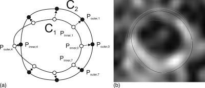
Figure 2a shows two wall segmentations on the same image slice: One is the result of the forward propagation and the other was produced by the backward propagation. Each contour was radially sampled with 45° intervals, resulting in eight sample points. The curve with sample points marked as hollow circles is denoted as C1 and that with sample points marked as black dots is denoted as C2. For the ith pair of corresponding points, one of the two points on one contour must lie inside the other contour, which is denoted as Pinner,i, and the other point is denoted by Pouter,i. We sampled the line connecting Pinner,i to Pouter,i into 10 uniform intervals. Each sample point, pi, can be represented by a single parameter, r. We denote the coordinates of each sample point by pi(r), which is defined by:
| (9) |
In our case, since we sampled with 10 uniform intervals, r increases from 0 to 1 with a 0.1 increment. For each sample point, we calculated the following dot product, which we denote as Ci(r):
| (10) |
where u is the unit vector in the direction from Pinner,i to Pouter,i, Gim(pi(r)) is the two-component image gradient evaluated at the point pi(r). Ci(r) can be interpreted as the directional derivative of image intensity along the direction from Pinner,i to Pouter,i. We chose to be the that evaluates to the minimum Ci(r). The minimum point was chosen to be the boundary because the arterial wall is relatively bright, and thus, the intensity on the edge of the arterial wall should be sharply decreasing.
Figure 2.
Illustration of the final contour determination rule described in Sec. 2C3. (a) C1 and C2 are segmented in the forward and backward propagation respectively. For each pair of the 8 sampled points, the optimum boundary point was searched from Pinner,i to Pouter,i. (b) shows the contour segmented in the forward propagation (dark blue), backward propagation (orange) and the optimum contour (light blue) on an axial image. The semiautomatically segmented lumen boundary is also shown (red).
To ensure that the final outer wall boundary is smooth, was filtered by a smoothing kernel:
| (11) |
In our application, f−1 = f1 = 0.2 and f0 = 0.6. The final wall contour was then produced by interpolating the set of points using the Cardinal spline.22
Contour editing in curved planar reformatted (CPR) views
In more extreme cases in which the blood signal is not properly suppressed or the artery is severely stenosed, the slice-based algorithm described above may not work well and boundary editing may be necessary. Since manual editing introduces observer variability and takes time, a good manual editing mechanism should keep the user interaction to a minimum, while also providing flexibility. Our manual editing mechanism contains two major components: (1) Curve planar reformatted (CPR) views and (2) construction of smoothed contours in CPR views.
CPR views
A centerline is required to produce a CPR view. This centerline needs to be smooth for a continuous CPR view. We created a smooth centerline by taking the centroid of the lumen boundary of every tenth slice as an input to the Cardinal spline model. For each axial image slice, there is an intersection with this centerline, which we denote as Cn = (Cn,x, Cn,y) on Image Slice n. From Cn, Image Slice n was resampled at an angle θ and at an interval equal to the pixel size. The result was mapped to the CPR view according to the following equation:
| (12) |
where 0 ≤ m ≤ M and M + 1 is the total number of samples obtained in Slice n, 0 ≤ n ≤ N and N + 1 is the total number of image slices in the 3D image, F is the CPR view, In is Image Slice n, and p is the pixel size.
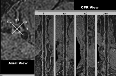
Four CPR views were generated with θ set to 0, π/4, π/2, and 3π/4. Figure 3 shows these four views in the right panel. In this figure, one of the contours in the π/2-view was selected and highlighted by red markers. The corresponding point being edited was also highlighted in the axial view with a red marker.
Figure 3.
The CPR editing tool. The left panel shows the axial view of a femoral artery 3D MERGE image. The right panel shows the CPR views resampled at 0, π/4, π/2, and 3π/4. The white lines represent the position of the displayed axial/CPR views.
Contour reconstruction and editing in CPR views
The lumen and outer wall boundaries were mapped to the CPR views according to the transformation described in Eq. 12. After the transformation, we smoothed each contour on the CPR views using the Gaussian kernel Gσ,L where σ is the standard deviation of the kernel, which is defined inside [−L, L]. Let X[n] be the x-coordinate when the y-coordinate equals n before smoothing. Except at control points (i.e., those marked with a red marker in the π/2-view in Fig. 3) that were not smoothed, the x-coordinates of the contours after smoothing, denoted by , were obtained using the following equation:
| (13) |
where . Dividing by this normalization factor ensures the sum of weighting factors in Eq. 13 equals 1. This operation is just the convolution operation with the boundary conditions considered.
Every tenth point of the contour was assigned to be a control point, and L in Eq. 13 was assigned to be 5. In addition, the first and last points were also assigned as control points. Once a user edits the control points on a CPR view, the edited contour is updated on the axial view immediately. In the CPR views, the control points are not smoothed by Eq. 13 to give the user the flexibility to move the control points. Not smoothing the contours at control points also causes the user to pay attention to the location where the accuracy of the semiautomated segmentation is problematic. At control points where a semiautomatically segmented contour is discontinuous on a CPR view, a user would pay extra attention to determine whether the contour is accurate or not. Thus, in addition to serving as an efficient editing tool, the CPR views also allow the continuity of the contours to be readily assessed and draw immediate attention to discontinuous points.
EXPERIMENTAL METHODS
Study subjects
We used six 3D MERGE images acquired for five subjects to evaluate our algorithm. We evaluated the left and right arteries of one subject, while evaluating only one side of the remaining five subjects. These subjects were symptomatic with intermittent claudication.
3D MERGE acquisition and reslicing
The 3D MERGE sequence was implemented using MSDE preparation and spoiled segmented FLASH readout with centric phase encoding.13 The femoral artery images were acquired using two stations with field-of-view (FOV) 400 × 40 × 250mm to cover up to 500mm longitudinally with isotropic voxel size of 1.0mm (zero-interpolated to 0.5mm). Total scan time was 7 min. The imaging parameters were TR = 10 ms, TE = 4.8 ms, flip angle = 6°, turbo factor = 100 and one excitation (NEX).
The current protocol provides coverage that includes the segment that is upstream from the femoral bifurcation. The image quality at this segment is poor. Thus, we focused our analysis on the superficial femoral artery starting from the femoral bifurcation and proceeding to the end of the femur. The entire length is approximately 300 mm. The region-of-interest was then resliced with an interslice distance of 1mm, resulting in approximately 300 axial images for each artery.
Metrics for comparison between two boundaries
Distance- and area-based metrics were used to compare two closed boundaries. We used these two sets of metrics to evaluate the lumen and outer wall boundaries separately.
Distance-based metrics
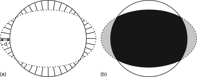
We measured distances of two contours on a point-by-point basis by first establishing a symmetric correspondence relationship23, 24 between them. The relationship is a one-to-one mapping between points on the two contours, which gives us a distance measurement dj at Point j [Fig. 4a].
Figure 4.
Illustration of the distance- and area-based metrics for comparing two closed boundaries. (a) Distance-based metrics: The symmetric correspondence relationship between two boundaries was first established. Each pair of corresponding points is associated with a distance measurement dj. Mean absolute difference (MAD) and maximum difference (MAXD) are the mean and the maximum distances respectively, calculated over all corresponding pairs. (b) Area-based metrics: Area overlap (AO) is the ratio of the overlapped area (black) to the total area enclosed by two boundaries expressed in percentage. Area difference (AD) is the percentage difference between the areas of two boundaries.
For each pair of contours, two parameters were computed to summarize the distance set obtained, where N is the total number of corresponding pairs: (a) mean absolute difference (MAD) and (b) maximum difference (MAXD), which are defined as follows:19
| (14) |
| (15) |
Area-based metrics
The area-based metrics compared the area enclosed by the contour representing the ground truth, which we denote as A1 here, and the area enclosed by another contour, which we denote as A2 [Fig. 4b]. We used two parameters to summarize the difference between the two contours: (a) the percent area overlap (AO) and (b) area difference (AD), which are defined as follows:19
| (16) |
| (17) |
Validation study
The validation study consisted of two parts. First, the accuracies of the lumen and outer wall boundaries were evaluated separately using the distance- and area-metrics described in Sec. 3C. The details of these comparisons are described in Sec. 3D1 for the lumen and Sec. 3D2 for the wall. Second, the ability of the segmentation approaches in extracting vessel wall thickness and area was assessed in Sec. 3D3.
Lumen segmentation and assessment
In the proposed segmentation method, lumen segmentation propagation was continually guided by an expert observer blinded from the manually segmented boundaries. This user guidance guaranteed that the lumen segmentation was reasonably accurate and further editing using the CPR views was therefore not performed. The arterial lumen was segmented by an expert observer on every tenth image. In order to assess the reproducibility of the algorithm, we segmented each image twice using different initial contours. The two sets of lumen boundaries were evaluated against the manual segmentation using the distance- and area-based metrics in Sec. 3C.
Wall segmentation and assessment
Because the vessel wall is sometimes in close proximity to and difficult to be separated from neighbouring muscle tissues, an expert observer segmented the vessel wall on every tenth image two times in order to assess the reproducibility of the manual segmentation. One segmentation was arbitrarily chosen as the gold standard (denoted by M1 hereafter). The remaining segmentation (denoted by M2 hereafter) was compared with M1 the same way as the semiautomatically segmented boundaries using the distance- and area-based metrics introduced in Sec. 3C. Because even an expert observer may have difficulty in accurately segmenting the vessel wall in some locations, it is more reasonable to assess the semiautomatic segmentation accuracy in relation to the observer variability.
In order to assess the reproducibility of the vessel wall segmentation using the proposed algorithm, two semiautomatic segmentation trials were carried out. We denote the two repeated segmented wall boundaries as SB1 and SB2 hereafter. As described in Sec. 2C2, the vessel wall segmentation depends on the geometry of the previously segmented lumen boundary. Therefore, there are two sources of variability in outer wall segmentation: (1) The difference between the initial contours used to initialize the forward and backward propagations and (2) the difference between the two repeatedly segmented lumen boundaries produced in Sec. 3D1. The overall effect of these two sources of variability was quantified in Sec. 4.
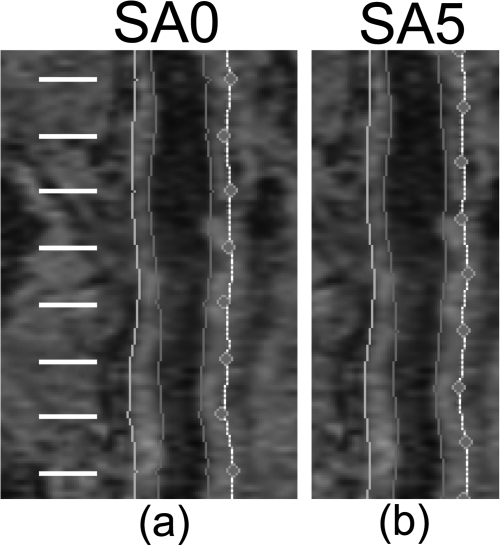
After the slice-based propagation was completed, the CPR-based editing was done by a user who did not have a knowledge about the manually segmented boundaries. We compared the semiautomatically segmented vessel wall produced with CPR-based editing (denoted by SA0) and SB1. Comparing the distance- and area-based metrics associated with these two methods allowed us to assess the degree to which the CPR-based editing tool improved segmentation accuracy. For SA0, the control points on the CPR views were located on slices where manual segmentation was performed [Fig. 5a]. Therefore, only contours edited by an expert observer were evaluated. In order to evaluate the segmentation accuracy at slices between control points, we also set the control points at the midpoint between two manually segmented slices [Fig. 5b]. The axial slices evaluated in this case were at least 5 slices away from any control point. The vessel wall segmentation produced in this way is denoted by SA5.
Figure 5.
Control points in the CPR views were set at (a) axial slices where manual segmentation was performed in SA0 and (b) the midpoint between two adjacent manually segmented axial slices in SA5. Manual segmentation was performed on every tenth axial slice. White lines represent the location of axial slices where manual segmentation was performed. The purpose of editing at the midpoints was to evaluate segmentation accuracy at slices that were not directly edited.
In summary, six vessel wall boundaries were produced – two manually segmented and four semiautomatically segmented boundaries:
M1, M2—Two repeated manual segmentations. M1 was arbitrary chosen as the gold standard. Comparing these two segmentations gives an assessment of variability of manual segmentation.
SB1, SB2—Two repeated segmentations produced by our proposed slice-based propagation. No CPR-based editing was performed.
SA0, SA5—Two different methods of editing the results produced by SB1 using the CPR views. In SA0, the editable control points are located on slices where manual segmentation was performed. In SA5, the control points are located at the midpoint between two manually segmented slices (Fig. 5).
Evaluation of vessel wall thickness and area
The main purpose of the development of a semiautomated segmentation technique for the peripheral arteries is to assess plaque burden. Therefore, in addition to evaluating the lumen and the outer wall boundaries independently, arterial wall area and wall thickness produced using different methods were also compared.
As described in Sec. 3D2, manual segmentation of the outer wall boundaries was performed twice (i.e., M1 and M2), one of which was considered gold standard (i.e., M1). To fairly capture the observer variability of vessel wall thickness and area measurements, lumen boundaries were manually segmented once more. Three parameters were computed for the six boundaries described in Sec. 3D2 on a slice-by-slice basis: (a) mean thickness (tmean), (b) maximum thickness (tmax), and (c) area (WA) of the wall. tmean and tmax were obtained in the same way as MAD and MAXD, except that, here, the symmetric correspondence relationship was established between the lumen and outer wall boundaries. WA is the area enclosed by the lumen and outer wall boundaries.
Then, two different analyses were performed. First, for each of the five nongold-standard boundaries (i.e., M2, SB1, SB2, SA0, and SA5), (a) mean thickness difference (Δtmean), (b) maximum thickness difference (Δtmax) and (c) wall area difference (ΔWA), were computed on a slice-by-slice basis by subtracting the measurement associated with M1 from the corresponding measurement for these five boundaries. Mean and the standard deviation of these differences were reported. These differences were also assessed by the Bland-Altman analysis.25 Another important metric to consider is the root-mean-square error (RMSE), which can be computed by taking the root of the sum of the square of the standard deviation and the square of the bias. Second, the measurements associated each of the four nongold-standard methods were compared with those of M1 using the correlation coefficient (r).
RESULTS
Evaluation of wall and lumen boundaries
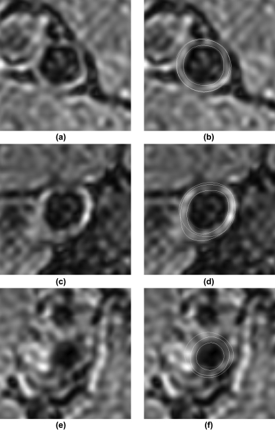
Table TABLE I. shows the distance- and area-based metrics associated with the two semiautomatically segmented lumen boundaries. Table TABLE II. shows the distance- and area-based metrics associated with the five nongold-standard outer wall boundaries. Figure 6 shows the segmentation results for three sample slices. The first, second, and third row show examples with good, average and lower than average segmentation accuracy respectively. The left column shows the original images and the right column shows the corresponding images with segmented contours superimposed. Yellow contours represent manual segmentation. Blue and red contours represent semiautomatically segmented wall and lumen boundaries, respectively, using Method SA0.
Table 1.
The average and the standard deviation of the distance- and area-based metrics associated with two repeated lumen segmentations with registration applied (Reg 1 and 2) and the lumen segmentation without registration (No Reg).
| MAD (mm) | MAXD (mm) | AO (%) | AD (%) | |
|---|---|---|---|---|
| Reg 1 | 0.20 (0.17) | 0.55 (0.48) | 85.60 (9.36) | 9.77 (9.78) |
| Reg 2 | 0.22 (0.19) | 0.56 (0.49) | 84.96 (10.88) | 10.55 (11.27) |
| No Reg | 0.23 (0.20) | 0.59 (0.51) | 84.46 (11.48) | 11.38 (15.85) |
Table 2.
The average and the standard deviation of the distance- and area-based metrics associated with wall boundaries produced by four methods (i.e., M2, SB, SA0, and SA5), as compared to the gold standard (i.e., first manual segmentation, M1). M2 represents the second manual segmentation. SB1 and SB2 represent two repeated semiautomatic segmentation boundaries without editing. SA0 and SA5 represent the semiautomatically segmented boundaries with editing. The difference between SA0 and SA5 was on the placement of control points on the CPR views (see Fig. 5).
| MAD (mm) | MAXD (mm) | AO (%) | AD (%) | |
|---|---|---|---|---|
| M2 | 0.21 (0.15) | 0.50 (0.39) | 89.39 (7.53) | 11.07 (12.25) |
| SB1 | 0.32 (0.23) | 0.77 (0.52) | 84.75 (9.46) | 12.90 (12.95) |
| SB2 | 0.32 (0.25) | 0.76 (0.55) | 84.65 (10.20) | 13.11 (13.22) |
| SA0 | 0.25 (0.14) | 0.60 (0.33) | 87.48 (6.51) | 9.69 (9.22) |
| SA5 | 0.30 (0.16) | 0.66 (0.34) | 85.44 (7.38) | 11.02 (10.08) |
Figure 6.
Segmentation results for three sample slices. The first, second, and third row show examples with good, average and lower than average segmentation accuracy respectively. (a), (c) and (e) show the original images. (b), (d) and (f) are the corresponding images with segmented contours superimposed. Yellow contours represent manual segmentation. Blue and red contours represent semiautomatically segmented wall and lumen boundaries, respectively, using Method SA0.
Two lumen and outer wall segmentation trials gave similar results, which are not statistically different in all categories. We have also investigated the effect of the registration-based propagation in lumen segmentation. Table TABLE I. shows the accuracy of lumen boundaries segmented without registration was only slightly lower than those produced with registration. This result is not unexpected because an expert observer was monitoring and revising the segmentation regardless of whether registration was applied. However, comparing to the algorithm with registration, the algorithm without registration requires the observer to edit the contours twice as many times, making the segmentation more tedious considering the coverage of the image.
The comparison between SB1 and SA0 indicated that editing on the CPR views has improved segmentation accuracy. In fact, although statistically significant, the results associated with M2 are close to SA0. The wall boundaries produced by SA5 were slightly less accurate than those produced by SA0.
Evaluation of vessel wall thickness and area
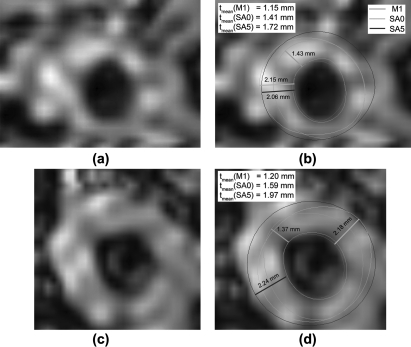
Table TABLE III. shows the difference between the vessel wall measurements associated with the five nongold-standard boundaries and those with the gold standard. The measurement bias associated with M2 was slightly lower than the semiautomated methods. The comparison between the measurements associated with SB1 and SB2 shows that the proposed semiautomated algorithm generated highly reproducible contours. Among the semiautomated methods, RMSEs of all measurements associated with SB1/SB2 were higher than those produced by other methods. The reduction of RMSEs associated with SA0 and SA5 comparing with SB1/SB2 shows that the segmentation accuracy was greatly improved after editing. The RMSEs of tmean and WA associated with SA0 and SA5 were similar, whereas RMSE(tmax) associated with SA5 was smaller than that with SA0. Because the outer wall contour produced by SA5 was interpolated from the two adjacent contours that user edited, it is usually more circular or regular than the contour produced by SA0. Even when the arterial shape was less continuous in the longitudinal direction and SA5 could not estimate the outer wall accurately, the inaccuracy did not have a significant effect in Δtmax because the contour shape produced by SA5 was more circular. In the two examples shown in Fig. 10, both SA0 and SA5 overestimated the size of the vessel wall and the overestimation was more severe in SA5 than in SA0. However, the difference in tmax between SA0 and SA5 was small and the difference in tmean was much greater. This explains why RMSE (tmax) associated with SA5 was smaller than that with SA0.
Table 3.
The average, standard deviation (in parenthesis in the first column) and root-mean-square error of the mean thickness difference (Δtmean), maximum thickness difference (Δtmax) and wall area difference (ΔWA) associated with four methods as compared to the gold standard (i.e., first manual segmentation, M1). M2 represents the second manual segmentation. SB1, SB2, SA0, and SA5 boundaries generated by semiautomatic segmentation methods (see caption of Table TABLE II.). tmean and tmax are expressed in mm and WA is expressed in mm2.
| Δtmean | RMSE(tmean) | |
|---|---|---|
| M2 | 0.197 (0.260) | 0.326 |
| SB1 | 0.224 (0.339) | 0.406 |
| SB2 | 0.229 (0.363) | 0.429 |
| SA0 | 0.225 (0.261) | 0.345 |
| SA5 | 0.233 (0.256) | 0.347 |
| Δtmax | RMSE(tmax) | |
| M2 | 0.273 (0.555) | 0.619 |
| SB1 | 0.389 (0.623) | 0.735 |
| SB2 | 0.395 (0.670) | 0.778 |
| SA0 | 0.434 (0.541) | 0.693 |
| SA5 | 0.364 (0.491) | 0.611 |
| ΔWA | RMSE(WA) | |
| M2 | 4.40 (4.92) | 6.60 |
| SB1 | 4.58 (7.10) | 8.45 |
| SB2 | 4.50 (7.46) | 8.71 |
| SA0 | 4.74 (5.29) | 7.11 |
| SA5 | 4.76 (5.46) | 7.25 |
Figure 10.
These two examples demonstrate the different properties of the maximum thickness (tmax) and the mean thickness (tmean) metrics. (a) and (c) show the original images of two image slices. (b) and (d) show the corresponding images with boundaries superimposed. The green contours in (b) and (d) represent the manual segmentation. The light and dark blue contours represent the outer wall boundaries produced using Methods SA0 and SA5 respectively. The semiautomated segmented lumen boundary is represented by the red contours. In these two examples, Method SA5 overestimated the vessel wall size more than Method SA0, which was reflected by the difference in tmean. However, tmax produced by the two methods were similar.
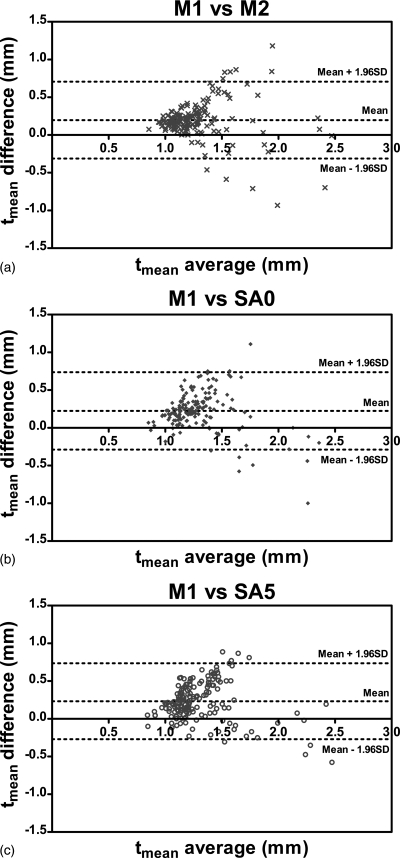
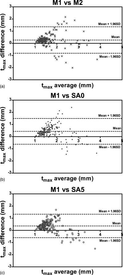
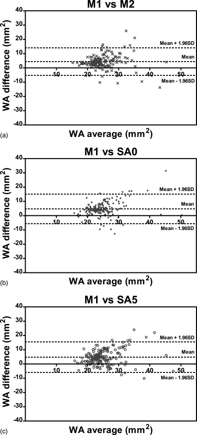
Figures 789 show the Bland-Altman plots of tmean, tmax and WA comparing three methods, SA0, SA5, and M2 with the gold standard M1. It can be observed from Figs. 78 that the automated algorithms (i.e., SA0 and SA5) tend to underestimate tmean and tmax if the average measurement is larger than a threshold, which is about 1.7 mm for tmean and about 2.5 mm for tmax. However, when the average tmean and tmax were smaller than the respective threshold, the automated algorithms tend to overestimate the wall thickness slightly. The bias of tmean and tmax were positive because in most cases, tmean and tmax were below the threshold.
Figure 7.
Bland-Altman plots of tmean comparing (a) M2, (b) SA0, and (c) SA5 with the gold standard M1. Difference values represent tmean of M1 subtracted from that of nongold-standard methods. Lines denoting the mean difference and ±1.96 SDs are also shown.
Figure 8.
Bland-Altman plots of tmax comparing (a) M2, (b) SA0, and (c) SA5 with the gold standard M1. Difference values represent tmax of M1 subtracted from that of nongold-standard methods. Lines denoting the mean difference and ±1.96 SDs are also shown.
Figure 9.
Bland-Altman plots of WA comparing (a) M2, (b) SA0, and (c) SA5 with the gold standard M1. Difference values represent WA of M1 subtracted from that of nongold-standard methods. Lines denoting the mean difference and ±1.96 SDs are also shown.
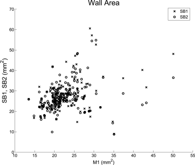
Table TABLE IV. shows that correlation coefficients between each of the three methods, M2, SA0 and SA5, and the gold standard M1 were around 0.6 for all three parameters, whereas the correlation between SB1/SB2 and M1 were much weaker. These results suggested that (1) the accuracy of the contours produced by SB1/SB2 had been greatly improved after editing, either by SA0 and SA5 and (2) the contours produced using SA0 or SA5 were about as close to those produced by the first manual segmentation (M1) as the contours produced by the second manual segmentation (M2). The difference between the correlation coefficients associated with SB1 and SB2 is greater than expected. Figure 11 shows a plot of the wall area measurements between SB1/SB2 and M1. The difference between the correlation coefficients associated with SB1 and SB2 can be explained by the few points with M1 area greater than 35 mm2. If these five data points were taken out, the correlation coefficients associated with the two trials are similar (0.36 for SB1 and 0.37 for SB2).
Table 4.
The correlation coefficients between the mean thickness (tmean), maximum thickness (tmax), wall area (WA) associated with four methods and the gold standard (i.e., corresponding measurements of the first manual segmentation, M1). M2 represents the second manual segmentation. SB1, SB2, SA0, and SA5 boundaries generated by semiautomatic segmentation methods (see caption of Table TABLE II.).
| tmean | tmax | WA | |
|---|---|---|---|
| M2 | 0.65 | 0.57 | 0.54 |
| SB1 | 0.39 | 0.36 | 0.38 |
| SB2 | 0.30 | 0.24 | 0.24 |
| SA0 | 0.61 | 0.55 | 0.60 |
| SA5 | 0.65 | 0.60 | 0.54 |
Figure 11.
Wall area measurement comparison between SB1/SB2 and M1. The difference between the correlation coefficients associated with SB1 and SB2 can be explained by the few points with M1 area greater than 35 mm2.
To compare the performance of SA0 and SA5, we performed two-side paired t-tests for tmean, tmax and WA. We found that the mean paired differences in tmean and WA between the two methods were not statistically significant, whereas the mean paired difference in tmax was statistically significant with P = 0.005. This result is not unexpected based on our previous analysis of the nature of the tmax metric using the examples in Fig. 10.
Time requirement and implementation details
Lumen segmentation for a femoral artery dataset with 300 slices took 2–3 min. The forward and backward propagation performed to segment the arterial wall took 40 s each, with the final boundary detection step taking another 30 s. Editing the outer wall boundary on the CPR views took about 3–4 min. The time required depends on the difficulty in separating the vessel wall from the neighbouring muscles. The algorithm was implemented in the Visual Studio C++ environment and made use of the Microsoft Foundation Class (MFC) library. The Visualization Toolkit (VTK) library26 was used in the construction of CPR views. All experiments were performed using an Intel® Xeon® 2.0 GHz CPU with 2.0 GB memory. In contrast, manually segmenting the lumen and outer wall boundaries for a femoral artery dataset on every tenth axial slice (i.e., a total of 30 slices per image) took about 70–80 min. Thus, segmenting the entire image using the semiautomated algorithm took a maximum of 10 min, whereas it would take a minimum of 700 min to segment the whole image manually.
DISCUSSION AND CONCLUSION
With the advent of fast 3D high-resolution MR imaging, it is now possible to image the whole femoral artery with submillimeter resolution in a few minutes. A semiautomated technique for analyzing such huge image sets efficiently is necessary for this 3D imaging technology to be used in the management of PAD. To address this need, we developed a semiautomated segmentation technique that consists of two basic components: (1) 2D slice-based 3D segmentation and (2) editing on the curved planar reformatted (CPR) views.
In our 2D slice-based 3D segmentation approach, the first contour on the series was manually segmented. Then, this contour was propagated to its adjacent image slice to serve as the initial contour, which was then refined using a deformable contour model previously described.14 In this paper, we introduced three innovations to the existing 2D slice-based segmentation approach: (1) In segmenting the lumen, we used a registration module to transform the final contour of the previous slice before it was used as the initial contour on the next slice in order to improve the initial contour (Sec. 2B). (2) We developed a propagation mechanism in which users can edit the lumen contour to prevent the algorithm from running off course (Sec. 2B). (3) To improve the accuracy of the wall boundary segmentation, we introduced a two-pass process in which the 2D slice-based segmentation propagated once forward and once backward, resulting in two contours on each axial image. Then, on each axial image, a gradient-based boundary decision process was used to determine the final contour based on the two contours (Sec. 2C).
However, there are some disadvantages in using the 2D slice-based segmentation approach to handle 3D datasets. First, the 2D slice-based approach does not enforce continuity of the contours in the longitudinal dimension. Second, it does not allow efficient manual contour editing. To address these drawbacks, we developed a manual editing mechanism in which user interactions take place on multiple CPR views (Fig. 3). Continuity along the longitudinal direction was enforced by smoothing the contours on the CPR views with the Gaussian kernel, except at control points (Sec. 2D2). This exception does not only give users flexibility to move control points; it also allows the continuity along the longitudinal dimension to be readily inspected and assessed at control points. Attention is drawn to the discontinuous control points and the user can choose whether and by how much the control points should be changed.
We used a set of distance- and area-based metrics to evaluate the segmentation accuracy of the proposed algorithm. First, we evaluated the lumen and outer wall boundaries individually. Second, we assessed four semiautomatically segmented boundaries (i.e., SB1, SB2, SA0, and SA5) by comparing their associated mean, maximum thickness, and the area of the vessel wall (i.e., the region enclosed by the lumen and outer wall boundaries) with the gold standard. We found that editing, either using SA0 or SA5, greatly improved the accuracy of the vessel wall size estimation. Although SA0 and SA5 overestimated the size of the vessel wall size as compared to the gold standard, they produced contours that were about as close to the first manual segmentation (i.e., the gold standard M1) as those produced by the second manual segmentation according to the RMSE reported in Table TABLE III. and the correlations reported in Table TABLE IV..
The difference in the results produced by SA0 and SA5 was interesting. In the evaluation of vessel wall thickness and area, paired t-tests showed that the mean paired differences in tmean and WA between SA0 and SA5 were not statistically significant, whereas the mean paired difference in tmax was statistically significant. The significant difference was largely due to the nature of the tmax metric as demonstrated in Sec. 4B and Fig. 10. This result, however, is in disagreement with Sec. 4A, where we reported that the outer wall boundaries produced by SA5 were less accurate than those by SA0. We confirmed by paired t-tests that the differences in the four distance- and area-based metrics associated with SA0 and SA5 were all statistically significant. This apparent paradox is resolved by the fact that lower outer wall accuracy as measured by the distance- and area-based metrics does not necessarily imply less accurate vessel wall size estimation, even though the same lumen boundary was used in vessel wall size measurement. We observed that some outer wall boundaries produced by SA5 were different from the corresponding boundaries produced by SA0 by only a small shift. For SA5, the contours being evaluated were not edited directly, and were only indirectly affected by the move of the control points because of the continuity constraint in the longitudinal direction. When the longitudinal position of the artery changes quickly between two control points, our arterial model, which has its continuity enforced by the constraint, may not change quickly enough to align with the true boundary, resulting in a small shift with respect to the true boundary. This small shift, however, does not affect the vessel wall size measurements. Although this small shift may be the main cause of the statistically significant difference between the outer wall segmentation accuracy between SA0 and SA5, as measured by the four distance- and area-based metrics, the difference is not likely to be clinically significant (with mean difference ≈0.05mm in MAD and ≈2% in AO).
The evaluation results of SA0 and SA5 indicate that editing does not only improve accuracy of contours on axial slices that were directly edited on the CPR views, but also on slices between adjacent control points, because continuity in the longitudinal dimension was enforced by the CPR editing tool. Thus, improvement in segmentation accuracy for the whole 3D femoral artery dataset can be achieved by editing a relatively few number of control points.
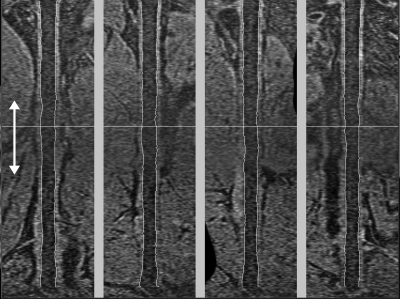
This study has shown that the vessel wall measurement error associated with the proposed segmentation method, as compared to the gold standard (i.e., M1), was about as large as the difference between two repeated segmentations performed by the same observer. However, the correlations with the first segmentation (i.e., M1) either for the second segmentation (i.e., M2) or semiautomated methods with editing (i.e., SA0, SA5) shown in Table TABLE IV. were relatively low (∼0.6 for all parameters). This can be attributed to two factors. First, the correlation coefficient is sensitive to the distribution of the measurement being made. A wider range in a measurement will lead to a better correlation, even if the RMSE is the same. The Bland-Altman plots of tmean, tmax and WA (Figs. 789) all indicate that the measurements are clustered in a small range. Second, the quality of the femoral artery images with current sequence parameters was suboptimal. Although good blood signal suppression has been reported for the use of 3D MERGE technique in carotid imaging,12 the flow velocity in femoral arteries is much lower and the use of 3D MERGE technique has not been optimized for peripheral artery imaging. Improvement in blood suppression in femoral artery images will make the semiautomated segmentation of the lumen boundaries faster and more accurate. Since the initialization of the outer wall boundaries depends on the lumen boundaries, improvement in blood suppression will also have an effect in the segmentation accuracy of the wall boundaries and the overall plaque burden estimation. In addition, the contrast of different tissue types was particularly low in the middle of the image (see Fig. 12). This was due to the fact that two separate stations were used to obtain the long coverage necessary to assess the femoral artery, and the SNR was lower at the overlapping regions between the two stations. Thus, improvements are warranted for the positioning of the two stations to minimize the SNR drop in the overlapping region. Accuracy and reproducibility of both manual segmentation and the proposed semiautomated algorithm will improve with the improvement in image quality. However, it should be emphasized that the goal of the proposed algorithm is less about improving accuracy of manual segmentation, but more about improving efficiency of plaque burden analysis. The fact that the proposed algorithm produced contours with similar accuracy comparing to manual segmentation means that the improved efficiency did not negatively impact the accuracy.
Figure 12.
Illustration of the lower image contrast in the middle of a 3D MERGE femoral artery image. Two separate stations were used to obtain the longitudinal coverage, and the SNR was lower in the overlapping region between the two stations (white arrows).
The motivation for the proposed semiautomated segmentation algorithm stems from the need for an efficient quantification tool to assess plaque burden in a large black-blood femoral artery dataset. The proposed segmentation procedure takes about 8–10 min to process a longitudinal coverage of 300 mm of a 3D femoral artery dataset, which considerably reduces the analysis time compared with manual review. This tool allows for large cross-sectional analyses to evaluate the risk associated with increased plaque burden in the peripheral arteries and longitudinal studies to evaluate the correlation between the size of plaque burden and symptoms of PAD.
ACKNOWLEDGMENTS
This study is supported by the grant R44 HL070576 from the National Institutes of Health and City University of Hong Kong Start-up Grant No. 7200245.
References
- Belch J. J. F., Topol E. J., Agnelli G., Bertrand M., Califf R. M., Clement D. L., Creager M. A., Easton J. D., Gavin J. R., Greenland P., Hankey G., Hanrath P., Hirsch A. T., Meyer J., Smith S. C., Sullivan F., and Weber M. A., “Critical issues in peripheral arterial disease detection and management: a call to action.,” Arch. Intern. Med. 163, 884–892 (2003). 10.1001/archinte.163.8.884 [DOI] [PubMed] [Google Scholar]
- Ouriel K., “Peripheral arterial disease,” Lancet 358, 1257–1264 (2001). 10.1016/S0140-6736(01)06351-6 [DOI] [PubMed] [Google Scholar]
- Criqui M. H., Langer R. D., Fronek A., Feigelson H. S., Klauber M. R., McCann T. J., and Browner D., “Mortality over a period of 10 years in patients with peripheral arterial disease.,” N. Engl. J. Med. 326, 381–386 (1992). 10.1056/NEJM199202063260605 [DOI] [PubMed] [Google Scholar]
- Glagov S., Weisenberg E., Zarins C. K., Stankunavicius R., and Kolettis G. J., “Compensatory enlargement of human atherosclerotic coronary arteries,” N. Engl. J. Med. 316, 1371–1375 (1987). 10.1056/NEJM198705283162204 [DOI] [PubMed] [Google Scholar]
- Vink A., Schoneveld A. H., Borst C., and Pasterkamp G., “The contribution of plaque and arterial remodeling to de novo atherosclerotic luminal narrowing in the femoral artery.,” J Vasc. Surg. 36, 1194–1198 (2002). 10.1067/mva.2002.128300 [DOI] [PubMed] [Google Scholar]
- Li F., McDermott M. M., Li D., Carroll T. J., Hippe D. S., Kramer C. M., Fan Z., Zhao X., Hatsukami T. S., Chu B., Wang J., and Yuan C., “The association of lesion eccentricity with plaque morphology and components in the superficial femoral artery: a high-spatial-resolution, multi-contrast weighted CMR study,” J. Cardiovasc. Magn. Reson. 12, 37 (2010). 10.1186/1532-429X-12-37 [DOI] [PMC free article] [PubMed] [Google Scholar]
- Isbell D. C., Meyer C. H., Rogers W. J., Epstein F. H., DiMaria J. M., Harthun N. L., Wang H., and Kramer C. M., “Reproducibility and reliability of atherosclerotic plaque volume measurements in peripheral arterial disease with cardiovascular magnetic resonance,” J. Cardiovasc. Magn. Reson. 9, 71–76 (2007). 10.1080/10976640600843330 [DOI] [PMC free article] [PubMed] [Google Scholar]
- Yuan C., Mitsumori L. M., Beach K. W., and Maravilla K. R., “Carotid atherosclerotic plaque: Noninvasive MR characterization and identification of vulnerable lesions,” Radiology 221, 285–299 (2001). 10.1148/radiol.2212001612 [DOI] [PubMed] [Google Scholar]
- Hayashi K., Mani V., Nemade A., Silvera S., and Fayad Z. A., “Comparison of 3D-diffusion-prepared segmented steady-state free precession and 2D fast spin echo imaging of femoral artery atherosclerosis,” Int. J. Cardiovasc. Imaging 26, 309–321 (2010). 10.1007/s10554-009-9544-0 [DOI] [PubMed] [Google Scholar]
- Zhang Z., Fan Z., Carroll T. J., Chung Y., Weale P., Jerecic R., and Li D., “Three-dimensional T2-weighted MRI of the human femoral arterial vessel wall at 3.0 Tesla,” Invest. Radiol. 44, 619–626 (2009). 10.1097/RLI.0b013e3181b4c218 [DOI] [PMC free article] [PubMed] [Google Scholar]
- Wang J., Yarnykh V. L., Hatsukami T., Chu B., Balu N., and Yuan C., “Improved suppression of plaque-mimicking artifacts in black-blood carotid atherosclerosis imaging using a multislice motion-sensitized driven-equilibrium (MSDE) turbo spin-echo (TSE) sequence,” Magn. Reson. Med. 58, 973–981 (2007). 10.1002/mrm.v58:5 [DOI] [PubMed] [Google Scholar]
- Balu N., Yarnykh V. L., Chu B., Wang J., Hatsukami T., and Yuan C., “Carotid plaque assessment using fast 3D isotropic resolution black-blood MRI,” Magn. Reson. Med. 65, 627–637 (2011). 10.1002/mrm.22642 [DOI] [PMC free article] [PubMed] [Google Scholar]
- Balu N., Wang J., Zhao X., Hatsukami T., and Yuan C., “Targeted multi-contrast vessel wall imaging of bilateral peripheral artery disease,” Proceedings of the 18th Annual Meeting of ISMRM Stockholm, Sweden (2010).
- Kerwin W., Xu D., Liu F., Saam T., Underhill H., Takaya N., Chu B., Hatsukami T., and Yuan C., “Magnetic resonance imaging of carotid atherosclerosis: plaque analysis,” Top. Magn. Reson. Imaging 18, 371–378 (2007). 10.1097/rmr.0b013e3181598d9d [DOI] [PubMed] [Google Scholar]
- Wang Y., Cardinal H. N., Downey D. B., and Fenster A., “Semiautomatic three-dimensional segmentation of the prostate using two-dimensional ultrasound images,” Med. Phys. 30, 887–897 (2003). 10.1118/1.1568975 [DOI] [PubMed] [Google Scholar]
- Ding M., Chiu B., Gyacskov I., Yuan X., Drangova M., Downey D. B., and Fenster A., “Fast prostate segmentation in 3D TRUS images based on continuity constraint using an autoregressive model,” Med. Phys. 34, 4109–4125 (2007). 10.1118/1.2777005 [DOI] [PubMed] [Google Scholar]
- Kanitsar A., Fleischmann D., Wegenkittl R., Felkel P., and Gröller M. E., “CPR: Curved planar reformation,” VIS ’02: Proceedings of the conference on Visualization ’02, Boston, Massachusetts (IEEE Computer Society, Washington, DC, 2002), pp. 37–44.
- Ladak H. M., Mao F., Wang Y., Downey D. B., Steinman D. A., and Fenster A., “Prostate boundary segmentation from 2D ultrasound images,” Med. Phys. 27, 1777–1788 (2000). 10.1118/1.1286722 [DOI] [PubMed] [Google Scholar]
- Chiu B., Freeman G. H., Salama M. M., and Fenster A., “Prostate segmentation algorithm using dyadic wavelet transform and discrete dynamic contour,” Phys. Med. Biol. 49, 4943–4960 (2004). 10.1088/0031-9155/49/21/007 [DOI] [PubMed] [Google Scholar]
- Fleet D. J. and Weiss Y., “Optical flow estimation,” Handbook of Mathematical Models in Computer Vision, 239–258, Springer, New York: (2006). [Google Scholar]
- Underhill H. R. and Kerwin W. S., “Markov shape models: object boundary identification in serial magnetic resonance images,” Proceedings of the 14th Annual Meeting of ISMRM 829, Seattle, Washington (2006).
- Beatty J. C., Bartels R. H., and Barsky B. A., An Introduction to Splines for Use in Computer Graphics and Geometric Modeling (Morgan Kaufmann, San Mateo, CA, 1995). [Google Scholar]
- Papademetris X., Sinusas A. J., Dione D. P., Constable R. T., and Duncan J. S., “Estimation of 3-D left ventricular deformation from medical images using biomechanical models,” IEEE Trans. Med. Imaging 21, 786–800 (2002). 10.1109/TMI.2002.801163 [DOI] [PubMed] [Google Scholar]
- Chiu B., Egger M., Spence J. D., Parraga G., and Fenster A., “Quantification of carotid vessel wall and plaque thickness change using 3D ultrasound images,” Med. Phys. 35, 3691–3710 (2008). 10.1118/1.2955550 [DOI] [PubMed] [Google Scholar]
- Bland J. M. and Altman D. G., “Measuring agreement in method comparison studies,” Stat. Methods Med. Res. 8, 135–160 (1999). 10.1191/096228099673819272 [DOI] [PubMed] [Google Scholar]
- Schroeder W. J., Martin K., and Lorensen W., The Visualization Toolkit, an object-oriented approach to 3D graphics (Kitware Inc., New York, 2002). [Google Scholar]


