Using the Saccharomyces Genome Database (SGD) for analysis of genomic information

Abstract

Analysis of genomic data requires access to software tools that place the sequence-derived information in the context of biology. The Saccharomyces Genome Database (SGD) integrates functional information about budding yeast genes and their products with a set of analysis tools that facilitate exploring their biological details. This unit describes how the various types of functional data available at SGD can be searched, retrieved, and analyzed. Starting with the guided tour of the SGD Home page and Locus Summary page, this unit highlights how to retrieve data using YeastMine, how to visualize genomic information with GBrowse, how to explore gene expression patterns with SPELL, and how to use Gene Ontology tools to characterize large-scale datasets.

The Saccharomyces Genome Database (SGD; http://www.yeastgenome.org/) is a comprehensive web-accessible resource for genetics and molecular/cell biology of the yeast Saccharomyces cerevisiae. SGD was started by David Botstein and colleagues at Stanford University in 1993 with a mission to collect and organize biological information about yeast genes and proteins, and make it available to the research community in a manner that facilitates retrieval and understanding in a consistent, user-friendly form (Cherry et al., 1997). The primary source of that information was the scientific literature, and SGD developed methods and policies of extracting data from publications. The identification of important information is performed by skilled individuals called curators. The curators’ actions are referred to as curation. The curation paradigm includes unbiased incorporation of results that have been subjected to the peer-review process and that can always be traced to their original source, usually a publication in a scientific journal. The data are linked to specific genes and presented in a way that provides an overview of a gene’s structure, the functions of its product and the locations where it acts. To ensure that data are processed accurately and consistently, curators must be trained, Ph.D.-level scientists with experience in molecular and cellular biology and yeast genetics. As research moves forward, and new types of data become available, new interfaces and new analysis tools are constantly under development (Engel et al., 2010).

Model Organism Databases (MODs) provide information in standardized forms to promote sharing of knowledge and its reuse. The major component used by MODs are controlled vocabularies, or ontologies, that describe a variety of biological observations. As with all MODs SGD uses the Gene Ontology (http://www.geneontology.org; GO; UNIT 7.2), as the main vocabulary for capturing different aspects of gene product function. GO is a system of standardized terms and their relationships that describe a primary activity of the gene product or its molecular function, a broader cellular role or involvement in a biological process, and the predominant localization, such as a protein complex, a subcellular structure, or an organelle (Harris et al., 2008). SGD captures mutant phenotypes using the Ascomycete Phenotype Ontology (APO), a vocabulary developed at SGD that has since been adopted by other fungal databases (Costanzo et al., 2009).

Over the past two decades, technological advances in DNA sequencing and the emergence of high-throughput techniques for exploring gene functions have changed the landscape of biology. Development of methods for large-scale gene expression analysis, automated mutant phenotype scoring, or high-throughput protein-protein interaction detection, has made it possible to investigate biological processes on a genome- and proteome-wide scale, thus laying a foundation for the systems biology approach. SGD offers a number of tools that provide access to large-scale datasets and facilitate retrieval of information for desired sets of genes and their analysis that takes advantage of the depth of gene-specific data.

As new experimental techniques are invented, and novel data analysis advances, the SGD resource will be updated with new tools and interfaces as needed. Here we introduce several tools offered by SGD that are designed to help in exploration and analysis of large-scale datasets. This is a guide to only a few features at SGD, and users are encouraged to explore the website on their own to discover others features and data types. Basic Protocol 1 introduces the SGD Home Page. Basic Protocol 2 is a guided tour through the Locus Summary page, the central unit of organization in SGD. Basic Protocol 3 demonstrates how to search and retrieve data using YeastMine. Basic Protocol 4 shows how sequence data and functional information can be visualized with the GBrowse genome browser. Basic Protocol 5 introduces SPELL, the tool for exploring gene expression data. Basic Protocol 6 shows how to use the Gene Ontology Slim Mapper to find common functions, roles, or localizations within a list of genes.

Basic Protocol 1

Exploring the SGD Home Page

The SGD home page (http://www.yeastgenome.org/; Figure 1) is a common entry point to the web site. Its purpose is to provide a starting point for many of the features and tools, but also to offer a quick, at-a-glance overview of the most recent and noteworthy events concerning SGD enhancements and yeast research. The Search box serves as a gateway to the variety of data types provided. Various tools related to data retrieval, analysis, and submission, as well as tools for investigator interactions, are accessible via the links at the top of the home page. Also, information on how to contact SGD staff and how to interact via social media (Twitter, Facebook, LinkedIn) is available there. Finally, the home page provides links to extensive documentation. These features are also accessible via hyperlinks, often context-sensitive, from within many parts of the website.

Figure 1.

The SGD home page (http://www.yeastgenome.org) provides access to most features of the website through the gene or keyword search box at the top of the page, as well as from links to data analysis tools, download data directories, and community information.

(Note: the layout of this page is currently under development; updated figure will be supplied within a few weeks)

Necessary Resources

Hardware

Device with access to Internet

Software

The website is compatible with current browsers, including: for Windows, Firefox (v2 or higher), Internet Explorer (v6 or higher); for Mac OS X, Safari (v2 or higher), Firefox (v2 or higher); for Linux, Firefox (v2 or higher).

Performing a simple search

1. Access the home page (http://www.yeastgenome.org/) and type your query into the “Search” box (Figure 1). The query text may be a gene or protein name, gene or protein symbol, gene or protein alias, author or individual name, or keywords and controlled vocabulary terms (such as a functional or phenotype ontology terms). The search is performed on a wide variety of data types and when there are multiple hits, a list of matches is displayed. For example, enter the word “bud” in the search box and start the search. The ensuing list of hits includes a number of Gene names, Descriptions, Name descriptions, Paragraphs, and Notes, all of which contain the word “bud” or a word that contains “bud” within it (such as “budding”). In addition, several GO terms contain “bud”, as do a number of phenotype terms. More versatile search capability is available through the YeastMine tool (see Basic Protocol 3).

Basic Protocol 2

Reviewing gene-specific information on the Locus Summary page

From the user perspective, the central unit of the database is the Locus Summary page. This is where the user can find the most up-to-date outline of what is known about a gene (Figure 2). In addition to protein-coding genes, various other chromosomal features have Locus Summary pages. This includes genes encoding various RNA species (tRNA, rRNA, snRNA, etc), as well as, centromeres, telomeres, transposons, and others. The information about the features is presented in several tabbed sections, with tabs arranged at the top of the page. Typically, for a protein-coding gene, the tabs show details of Gene Ontology annotations, mutant phenotype data, genetic and physical interactions, gene regulation, protein properties, and other resources. Select the various tabs and you will see more information. The content of the tabs is described below.

Figure 2.

The Locus Summary page displays the outline of the current knowledge about the gene. More detailed information is available by selecting one of the tabs near the top of the page.

(Note: the layout of this page is currently under development; updated figure will be supplied within a few weeks)

Necessary Resources

Hardware

Device with access to Internet

Software

The website is compatible with current browsers, including: for Windows, Firefox (v2 or higher), Internet Explorer (v6 or higher); for Mac OS X, Safari (v2 or higher), Firefox (v2 or higher); for Linux, Firefox (v2 or higher).

Overview of the Locus Summary page

1. The Summary page is the default tab displayed as a result of a successful search for a unique gene name. This is also the page to which various tools throughout the website point when referring to individual genes. The Summary page is divided into several sections to help you to easily find the right information. Some of these sections are described below.

   1. Basic Information

      The basic information on the Locus Summary page includes the names under which the locus is referred to in the literature. The Standard Name is a primary name (sometimes called the gene symbol by other organismal communities) in SGD, typically reflecting a known or presumed function and based on naming guidelines agreed upon by the budding yeast research community. The Systematic Name is a standardized designation given to the locus during the chromosome sequencing stage. Other names that are found in the literature are listed as aliases. The section also contains a text description that summarizes the function, biological significance, and other important features of the locus in a concise, headline-like format.

   2. Functional information

      The functional information on the Locus Summary page is presented as GO annotations, controlled-vocabulary terms that describe the molecular function the gene product performs, the biological process to which it contributes, and the cellular component in which it is found. The functional information may also include mutant phenotypes, and physical and genetic interactions. All this information is presented in a concise form to give quick at-a-glance overview. Each piece of information, however, is linked to another page that provides more details.

   3. Sequence Information

      The sequence information contains the features of the nucleotide sequence and the current gene structure, including the chromosomal position of the locus and the number of exons and introns, along with their chromosomal sequence coordinates. Hyperlinks lead to other pages that display the genomic sequence, the coding sequence, or the translation product.

2. The Locus History tab provides an overview of how the nomenclature and sequence annotations of the locus have changed. This includes any gene name changes, past updates to the nucleotide sequence, and any gene structure improvements. Each piece of information is referenced to a source, usually the published literature.

3. The Literature tab shows a compilation of references that contain information relevant to the locus. Each citation contains the authors, title, bibliographic data, and the hyperlinked names of other genes addressed in the paper; it also contains buttons that link to either the SGD Curated Paper page or the Pubmed record at NCBI, each of which contains the text of the abstract. There is also a button to access full-text articles, where available. SGD classifies the papers by literature topics, based on the papers’ primary focus. The SGD Curated Paper page contains the topics assigned to each paper. The list of the topics assigned to the total group of references for a locus is shown on the left side of the Literature Guide page for that locus. In order to see only papers that focus on a particular topic, click on that topic in the list. For example, click on “Mutants/Phenotypes” to see the list of references that analyze mutants and phenotypes.

4. The Gene Ontology tab presents the details of the GO annotations. The information is displayed in three sections, one for each annotation method, and in tables for each GO aspect (molecular function, biological process and cellular component). Each annotation is accompanied by additional information, such as evidence codes that indicate what type of data supports the annotation, and the reference(s) on which the annotation is based.

   1. Annotation methods

      Manual curation of the data for individual genes from published literature yields GO annotations classified as “Manually curated”. Since these annotations are supported by peer-reviewed experiments and carefully evaluated by a trained curator, they are considered the highest quality annotations. “High-throughput” annotations are assigned based on large-scale, often genome-wide experiments. Even though the experimental design and techniques are subject to the peer-review process and manual curation, each annotation may not be individually reviewed. All functional predictions incorporated into SGD from external sources are classified as “Computational” annotations. These annotations are generated using algorithms developed by bioinformatics groups and are not manually reviewed.

   2. GO Evidence

      Evidence codes are a mandatory part of each GO annotation. Their purpose is to indicate what type of data serves as the basis for the annotation, and thus, the confidence level that needs to be applied in evaluating the annotation. The Gene Ontology Consortium provides an ample vocabulary of evidence codes that covers various types of experimental results (e.g., IDA – Inferred from Direct Assay, or IMP – Inferred from Mutant Phenotype), as well as computational predictions (e.g. ISS - Inferred from Sequence or Structural Similarity, or ISO -Inferred from Sequence Orthology). To access a detailed guide to GO evidence codes, click on the hyperlinks in the Evidence column.

   3. “Assigned on” and “Last Review” dates

      An important factor in evaluating a GO annotation is whether it reflects current developments in the field. Each GO annotation therefore has a date stamp, a date when the annotation was assigned. Moreover, every GO Annotations page displays the date when a curator reviewed the entire set of manual annotations for that particular gene.

   4. GO Term page

      Clicking on any GO term in the GO Annotations table opens a GO Term page. The page contains a definition of the term as maintained by the Gene Ontology Consortium. Clicking on one of the icons next to View Ontology opens either a graphical or text-only ontology tree, which shows the parentage of the current term, as well as all the descendant terms, and allows navigation through the ontology branches. The page also provides a table of all genes that share this GO term. Click on the “download data” link to receive these data as an Excel spreadsheet. There are also two items worth exploring under Links to Additional Annotations: you can view annotations to this term in multiple organisms, or you can search SGD data for genes annotated to any term that is a descendant of this term.

5. The Phenotype tab contains details about phenotypes associated with mutations in the locus. Only phenotypes of single mutations are shown here (effects of double mutations are curated as genetic interactions). SGD uses a controlled vocabulary system (Ascomycete Phenotype Ontology, APO) to describe mutant phenotypes (Costanzo et al., 2009). Click on the “Browse phenotype terms” button to see the entire vocabulary. Clicking on a term in the phenotype table or in the browser returns a list of all genes in SGD associated with that phenotype. Names of the chemicals associated with phenotypes, such as drugs affecting growth or nutrients, are derived from the Chemical Entities of Biological Interest (ChEBI) database at the European Bioinformatics Institute (EBI) (Degtyarenko et al., 2009). Click on the chemical name to retrieve all genes with phenotypes that involve that chemical. In every case, the list of phenotypes for a particular gene, or the list of genes sharing a particular phenotype, can be downloaded in tab-delimited files.

6. The Interactions tab contains a table of the genetic and physical interactions that have been demonstrated for the locus, with references for those experiments shown in the right-most column. These data are annotated by curators from the BioGRID project (http://thebiogrid.org/), and are imported into SGD (Stark et al., 2011). The data in the table can be sorted and filtered; double-clicking on any cell brings up a menu of options. You can access a help page for manipulating the table via the link at the top of the page (click on “using the table”). There is also an option to view the table as plain text. Note that all the interaction data can be downloaded or further analyzed using the tools at the bottom of the page.

7. The Expression tab opens a link to the gene expression analysis tool, SPELL, described in more detail in Basic Protocol 5.

8. The Protein tab, present on Locus Summary pages of protein-coding genes, gives access to protein information such as the predicted molecular weight, isoelectric point, amino acid composition, and other physico-chemical properties that are calculated based on the primary sequence. The page also contains a diagram of domains and motifs identified in the protein sequence. Click on the diagram to access an expanded, interactive view. More information about the protein is available through links to many external resources, including the protein modification database PhosphoGRID (Stark et al., 2010), the protein signature database InterPro (Hunter et al., 2009), and others. Explore information and links available on three sub-tabs (Protein Info, Domains/Motifs, Physico-chemical Properties) for the full range of protein-related information.

9. The Wiki tab leads to the public wiki page about the locus. The wiki pages were created to enable researchers to share unpublished or published information about the locus with others. We invite you to create an account and contribute to the wiki pages.

Basic Protocol 3

Using YeastMine to retrieve and analyze multiple data types for sets of genes

As SGD has incorporated an immense amount of data covering a variety of data types for the over 6600 S. cerevisiae genes, the need for a sophisticated yet straightforward tool to retrieve and compare data has become apparent. The InterMine system (http://www.intermine.org/), developed as an open source project by the Cambridge Systems Biology Centre, is a powerful tool for integrating multiple types of data from different sources into databases that can be accessed by web query tools from user-accessible interfaces (Lyne et al., 2007). Using InterMine, SGD has incorporated the S. cerevisiae data to create YeastMine, a powerful data warehouse and search tool (http://yeastmine.yeastgenome.org/). YeastMine allows for retrieval and analysis of chromosomal features, sequences, protein features, GO annotations, phenotypes, interaction data, and curated literature, and other data types will be added soon. Data can be accessed using pre-defined templates, or you can design custom queries and manipulate the output to organize suitable tables. All data can be easily downloaded. This protocol describes how to input a set of gene names to create a list within the tool, and then how to use pre-made templates or create your own templates to analyze that gene list for various types of data.

Necessary Resources

Hardware

Device with access to Internet

Software

The website is compatible with current browsers, including: for Windows, Firefox (v2 or higher), Internet Explorer (v6 or higher); for Mac OS X, Safari (v2 or higher), Firefox (v2 or higher); for Linux, Firefox (v2 or higher).

Constructing a query

1. Open the YeastMine home page (http://yeastmine.yeastgenome.org/). You can search individual gene identifiers or search keywords, but to retrieve information for a set of genes first create a list containing the gene identifiers (such as gene names) for that set and then use the list in queries with the pre-designed templates. In fact, a few templates run automatically when a gene list is created, to begin the process of data retrieval. Before you generate a list, though, create a MyMine account and log in so that any lists and analyses you do will be saved indefinitely. (If you don’t have a MyMine account, your lists and queries will be saved for use during the current session only.)

2. Creating a gene list

   To create a gene list, click on the “Lists” tab at the top of the YeastMine home page, select the “Upload” option at the left. Select the type; note that lists can be created from many different feature types or other data types. Type or paste in the gene identifiers, or upload them from a file. After you click “Create List”, you will be prompted to enter a name for the list. Decide on a list name, and click on the “Save a list..” button. A results table containing gene identifier information for the first 10 genes of the list appears (Figure 3A). Additional genes can be accessed by clicking the “Next” link below the table. If some identifiers don’t produce an exact match, an intermediate confirmation page will appear allowing you to resolve any ambiguities. Once on the results page, scroll down below the table to see analyses of your gene list. Creation of the list triggers pre-made queries (templates) – in this case chromosome distribution, GO term enrichment, and publication enrichment – to run (Figure 3B). The data are presented as interactive widgets, and the templates used to retrieve that data are shown. Note that these templates are a subset of those accessible from the “Templates” tab at the top of each YeastMine page.

   Immediately below the table is a link for viewing all the records as results (Figure 3A). Clicking on this produces a larger table that contains options to add additional data, or to export this data. Try adding a column containing the Description for each gene. Click on “Add Column” and select “Gene > description” from the pull-down menu. Note that the new column appears on the right side of the table. The summary button at the top right of each column heading brings up a display for summary statistics for that column; for example, names and identifiers, and most non-numerical data, are counted, while numerical data are analyzed for the minimum value, the maximum value, the mean and standard deviation.

   When you have finished creating your lists, you can view and access them by moving from the “Upload” selection to the “View” selection. YeastMine also contains a set of pre-designed lists that SGD curators have generated for users. You can compare lists to each other using the “Actions” options.

3. Using templates to perform queries

   To look at the full list of templates, click on that tab. (You can also select a category of templates from the “popular templates” section in the middle of the YeastMine home page.) Perhaps you want to retrieve the curated phenotype data in SGD for the set of genes in your list. You can filter out the templates that aren’t relevant by selecting the “Phenotypes” category from the “Filter” pull-down menu. Now the list only contains 2 templates: “Phenotype → Genes”, which shows all the genes annotated to phenotypes you select, and “Gene → Phenotype”, which shows all the phenotypes for specific genes you enter. The second template is the appropriate one for this query. Click on that link, and then check the box next to the words “constrain to be..” and finish the sentence with the appropriate information. Then click on “Show results”.

4. Using the QueryBuilder tool to edit or build new queries Finally, you can edit queries or create new ones with the QueryBuilder tool. (Remember to stay logged into MyMine so that your queries are saved.) Go back to the “Templates” page and open the “Gene → Phenotype” query. Click the “Edit Query” button to open QueryBuilder. The page shows the Model browser on the left (Figure 4A), an overview of the present query on the right (Figure 4B), and the columns that will show up in the results table at the bottom (Figure 4C). The Model browser allows you to find the fields to include (click “show” or “summary”) or constrain in the query. Scroll down the page and click on “Start building a template query”. As you set up a query, you will see the “Query Overview” and “Columns to Display” sections change as they incorporate your selections. Clicking on the “X” button removes the field. You can also choose the order of the columns by dragging the blue boxes to different positions.

   The description of the “Gene → Phenotype” query indicates that it includes data for Uncharacterized, Dubious, and Verified ORFs, as well as other feature types. Let’s create a new template in which we add constraints that exclude data for Uncharacterized and Dubious ORFs. In the Model browser, find the “qualifier” class and click “constrain”. The popup window will ask you to choose a filter; select “!=” (for “not equal to”) and type “dubious” in the box. Then click “Add to query”. This addition will show up in the query overview, under the Qualifier field. Repeat these steps, typing “uncharacterized” in the box this time. Scroll down to the “Building a new template query” section and update the fields to reflect your new query. Click “Update settings”. Now the template review will include your new name and description. Click “Save Template”, and then “Save query”, and then try using the template.

   Open the MyMine tab to look for your additions. The new template will be on the “Saved Templates” page, and, since you saved the query separately, the query from the template will appear on the “Saved Queries” page.

Figure 3.

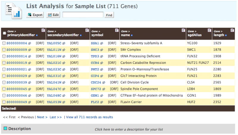
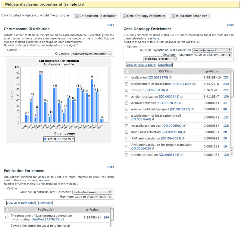
Data retrieval with YeastMine. A) Results table obtained after creating a sample gene list. The primary identifier is the SGDID for each gene, followed by the systematic name (referred to as the secondary identifier), followed by the standard gene name (called the symbol). Each of these is linked to the Locus Summary page for that gene. The fourth column, name, explains the 3-letter acronym used for the standard name. This is called the Name Description on the Locus Summary page. The fifth column, Alias names, contains other names used for the gene, besides the standard name. Additional rows of the table can be viewed by clicking on the “Next >” link below the table. B) Partial figure of the interactive widgets displaying properties of the sample list (note that the Publication Enrichment list is truncated). These displays were generated by YeastMine during creation of the list, by automatic running of several pre-made template queries. The Chromosome Distribution graph shows the number of genes in the list found on each chromosome (Actual) compared to the number expected to be found on each chromosome (Expected). Clicking on a bar in the graph generates the list of Actual genes on that chromosome. The Gene Ontology Enrichment table displays the BP, MF, or CC GO terms annotated multiple times for genes in the list, the number of times that term appears, and the p-value, which is the probability that that count occurs by chance. GO term IDs are linked to term pages of the AmiGO database. The Publication Enrichment table displays a similar arrangement of columns, except that publications used for annotation of the genes in the list, rather than GO terms, are counted. PubMed IDs are linked to the abstract of the paper from NCBI’s PubMed database.

Figure 4.

“Gene → Phenotype” query displayed in the QueryBuilder tool. A) The Model Browser displays the options of classes and attributes for building a query. Click on the “+” sign next to a class (such as “chromosome”) to display the attributes pertaining to that class. Clicking “summary” adds all the attributes of that class to the query. A single attribute can be restricted from the query by clicking “constrain”. Single attributes can be added by clicking “show”. B) The “Query Overview” displays the query as you build it. To remove an item, click on the red “X”. C) The “Columns to Display” section allows you to choose the content and order of the columns for the results table. Click on the red “X” to remove a column; drag the box to a different position to determine the order of the columns. (Note that in this figure the “Columns to Display” section from the “Gene → Phenotype” query has been truncated.)

Basic Protocol 4

Exploring genome features with GBrowse

The Generic Genome Browser (GBrowse; Unit 9.9) is a tool developed by Lincoln Stein (Stein et al., 2002) that allows overlying genomic sequence with functional annotations, thus enabling quick, visual access to genome features. The tool is easily expandable to accommodate the growing number of datasets. It is also customizable to serve specific needs of a user. The genomic sequence can be zoomed in to the level of the nucleotides, or zoomed out to visualize the entire chromosome. Different types of data are displayed as the horizontal sections in the display, called tracks, aligned with the sequence. The tracks depict known and predicted genes, open reading frames, gene models, and other chromosomal features (centromeres, telomeres, transposons). In addition, many types of genome-wide experimental data can be incorporated as GBrowse tracks including transcripts detected by RNA-seq (Yassour et al., 2009) or tiling array technologies (Xu et al., 2009), recombination hot spots (Mancera et al., 2008), and RNA polymerase occupancy data (Steinmetz et al., 2006) or sites of transcription factor binding by ChIP chip techniques (MacIsaac et al., 2005). Each track can be turned on or off individually, so that only tracks of interest are shown. SGD provides many tracks, with more tracks being regularly added. Using the BUD2 gene as an example, this protocol will show how to find a region of interest, how to explore various types of data associated with it, and how to save and share that information.

Necessary Resources

Hardware

Device with access to Internet

Software

The website is compatible with current browsers, including: for Windows, Firefox (v2 or higher), Internet Explorer (v6 or higher); for Mac OS X, Safari (v2 or higher), Firefox (v2 or higher); for Linux, Firefox (v2 or higher). Some features of GBrowse require javascript and cookies to be turned on.

Searching for a chromosome region

• 1.GBrowse is accessible through a hyperlink from SGD home page (http://browse.yeastgenome.org/), but also via a thumbnail image on each Locus Summary page. On the GBrowse page enter “BUD2” into the text field below the label “Landmark or Region:” and click the “Search” button. The browser will show the region of Chromosome 11 containing the gene named BUD2. Select “Show 20 kbp” from the pulldown “Scroll/Zoom” menu in the Search panel to see a larger genomic context. By default, the browser displays all annotated sequence features and protein coding genes, with the query gene highlighted in yellow (Figure 5).

  1. Searching for a landmark

     The types of designations that the tool recognizes are: a chromosome name (“chr4”), chromosomal coordinates (“chr01:123,000..160,000”), a gene name (“BUD2”), a systematic ORF name (“YKL092C”), an alias (“CLA2”). The search is not case-sensitive. The search box has an active autocompletion feature: when you start entering a gene name, a list of possible choices will drop down. You may also use a keyword (“budding”), or the wildcard character “*”. For example, a search for “bud*” will return genes, whose names, aliases, or descriptions contain the phrase “bud”. When the search returns multiple hits, you will be presented with a disambiguation screen that shows a diagram of all chromosomes with landmarks matching your query and a table with a list of hits. Clicking on one of the landmarks, either in the diagram or in the table, will bring that region to the Details panel of the browser.

  2. Keyword searches

     Keywords entered in the text field that are not recognized as landmarks are used for searches within the gene descriptions (see Basic Protocol 2). Searching for “ubiquitin”, for instance, will return a list of genes whose descriptions contain not only “ubiquitin”, but also partial word matches, such as “deubiquitination”, or “ubiquitinated”. Searching for multiple keywords will produce results as if the keywords were combined with the Boolean OR operator, e.g. a search for “ubiquitin ligase” will return a larger list of genes with descriptions containing either “ubiquitin” or “ligase”. More sophisticated searching is available elsewhere (see Basic Protocol 3).

  3. Search panel

     The Search panel of the browser window (Figure 5a) contains some of the navigation tools. Scroll left or right along the chromosome by clicking the greater-than or less-than buttons next to the “Scroll/Zoom” label. The double signs scroll an entire screen, while single signs scroll a half screen. In order to zoom in or out, use the “Show XXX kbp” pop-up menu. The number of base pairs selected in the menu is the length of the region shown in the Details panel. Adjustments to the zoom level can be made with the minus and plus buttons, which allow changes in 20% increments. Checking the “Flip” checkbox turns over the display in the Details panel, so that the minus strand is shown in reversed orientation. The search panel also provides access to several plug-ins that facilitate data download or analysis. Select an option from the pop-up menu, click “Configure…” to unfold a configuration panel, adjust the settings, and click the “Go” button.

  4. Overview panel

     The overview panel displays a schematic diagram of the entire chromosome (Figure 5b). The highlighted rectangle represents the region currently displayed in the browser. By default, it also displays some important landmarks, such as a centromere and genetic markers. The scale representing the chromosome can also be used for navigation: a single click on the scale re-centers the browser on the region surrounding the clicked location; a click-and-drag defines a new region to be displayed in the Details panel.

  5. Details panel

     With the default settings, the Details panel displays all annotated sequence features, including protein coding genes, tRNA and snRNA genes, transposons and LTRs, centromeres, telomeres, autonomously replicating sequences, and others (Figure 5c). The features are displayed as horizontal bars, with their orientation, where applicable, indicated by pointed ends. The characterized protein-coding genes are show in red, whereas uncharacterized genes and other features are shown in beige. Dubious features, those that are deemed unlikely to be real, are shown in grey. Depending on the zoom level, each feature may be accompanied by its name and a brief description. Mousing over a feature produces a text bubble with additional information. Clicking on a feature opens its Locus Summary page. The ruler at the top of the Details panel not only shows the scale, but also serves as a navigation tool. A single click re-centers the display on that location. Dragging along the ruler selects a region and opens a pop-up menu with options to zoom in, re-center, or dump the sequence of the selected region in a FASTA format. Many elements of the Details panel can be customized, as described in more detail below.

Figure 5.

GBrowse main window displaying a 20 kbp fragment of Chromosome 11 centered on the BUD2 gene (highlighted in yellow). The browser display is divided into several panels that provide (a) search and navigation tools, (b) overview of the region landmarks, and (c) details for selected tracks, including annotated chromosomal features, unannotated transcripts, and a graph depicting Pol II occupancy data.

Exploring the datasets

• 2.Click on the “Select Tracks” tab above the Search panel in order to access the list of available datasets. Each dataset is identified with a short name followed by the first author and the year of publication, e.g. “cDNA transcripts: Miura et al. (2006)” or “CUTs: Xu et al. (2009)”. The names are hyperlinked to a full citation and a brief summary of the experiments. Only published or soon-to-be published results are incorporated. Datasets are grouped in a multilevel list: datasets with similar types of information are listed under the same heading. For instance, datasets related to gene structure (introns, transcription start sites) are under “Gene Models”, various types of expression data are listed under “RNA Expression Profiling”, etc. You can select any number of desired datasets by checking boxes next to their names. You can also select or deselect entire groups by checking the “All on” or “All off” boxes. Locate the “ncRNA” heading and check “All on” in the “Tiling Array” subheading. Also select “Pol II occupancy: Steinmetz et al. (2006)” under “Transcription Regulation”. Click “Back to Browser” to see the results.
• 3.Selected datasets are displayed as tracks in the Details panel. Notice the presence of unannotated transcripts in the vicinity of BUD2, such as SUT665 (for Stable Unannotated Transcript), an antisense transcript on the opposite strand to MBR1 that starts in the region downstream from BUD2. Also notice a number of CUTs (Cryptic Unstable Transcripts). See how the Pol II (RNA polymerase II) occupancy graph correlates with known and unknown transcripts. The tracks can be put in any order by clicking on their names and dragging them to a desired location. More information about each feature, including the sequence, is available by clicking on its glyph or name. Navigate across the region using the Scroll/Zoom buttons. New tracks can be added at any time by clicking on the “Select Tracks” tab at the top, or “Select Tracks” button at the bottom.
• 4The display can be customized. The set of icons to the left of the track name provides additional controls. In order to declutter the browser, you can minimize a track by clicking on the “−” icon. To remove a track you no longer need, click on its “x” icon. To share the track with another user, click the “radio wave” icon: that will open a pop-up window with an URL that can be sent to a colleague, or used to export the track data to another instance of GBrowse. The “wrench” icon opens a configuration window that allows customizing many elements of the track appearance (style, color, height, etc). The “floppy disk” icon allows downloading the track data in the GFF format. You can choose to download data for the current region, for the current chromosome, or the entire dataset. The “?” icon provides the full citation, a brief description, and a Pubmed link for the dataset.

Basic Protocol 5

Using SPELL to analyze microarray gene expression data

Genome-wide outlook on gene expression is an indispensable element of the systems biology field, thus the microarray technology that allows fast and reliable screening of thousands of genes at a time has become an invaluable tool in the arsenal of modern biology. However, the vast quantities of gene expression data from microarray experiments pose a significant challenge in finding the most informative results among, ultimately, thousands of experiments and millions of individual data points. Our objective is to provide a clear and easy-to-use interface that facilitates expression analysis for genes of interest by identifying the most relevant experiments and by finding other genes that show the most similar expression pattern. SPELL (Serial Pattern of Expression Levels Locator) is a tool developed for this purpose by the Troyanskaya lab at Princeton University (Hibbs et al. 2007). Given a query gene, or genes, the tool ranks hundreds of datasets from published microarray experiments based on their relevance (correlation) to the query set and then identifies additional genes whose expression profiles most closely resemble those of the query gene(s). It then displays the results in a matrix where datasets and genes are provided in rank order, thus allowing quick visual identification of the most informative datasets and coregulated genes. In order to facilitate interpretation of the biological significance of such coordinately expressed genes, SPELL calculates which Gene Ontology terms are significantly enriched among them. This protocol explains how to perform a search and how to interpret the results.

Necessary Resources

Hardware

Device with access to Internet

Software

SPELL is compatible with current browsers, including: for Windows, Firefox (v2 or higher), Internet Explorer (v6 or higher); for Mac OS X, Safari (v2 or higher), Firefox (v2 or higher); for Linux, Firefox (v2 or higher). Many features of the tool require javascript and cookies to be enabled.

Constructing a query

• 1Go to the SPELL main page (http://spell.yeastgenome.org/). In the Gene Name(s) box, enter the name of your gene of interest. This has to be an unambiguous SGD gene name: a standard name, e.g. HRD1, a systematic name, e.g. YOL013C, or a unique alias, e.g. DER3. You may enter multiple gene names, separated by a space. In the “# Results” pull-down menu, select the number of similarly expressed genes you want to retrieve. The default value is 20, but it can be increased to 50 or 100. Click the Search button.

  1. Dataset Listing

     The main page also provides links to the Dataset Listing page which contains a catalog of publications from which the compendium of datasets currently available via SPELL searches has been obtained. For each publication, the table lists the first author’s name, a number of experimental conditions investigated, a brief description of the experiments, and a PubMed ID. A details link in the description leads to a full description that outlines the experimental designs and summarizes the major conclusions. Clicking on the PubMed ID link opens a PubMed abstract page from NCBI. The table can be sorted by any of the columns by clicking on the column heading.

  2. Show Expression Levels

     The Show Expression Levels link on the main page opens a tool that shows expression profiles for a query gene(s) in all datasets. The datasets are ordered alphabetically by their authors’ names and displayed in 10 per page installments that can be chosen from the “Datasets to view” pop-up menu. See later in the chapter for explanations of the profile display and options.

Analyzing the results

Results of the search are displayed in the form of a “heat map” (Figure 6). Datasets are presented as columns, 10 per page. To see other datasets, select a different range from the “Dataset to view” pull-down menu at the top of the page. Genes are shown as rows, 20 per page by default. To see more genes, select 50 or 100 from the “# of Result Genes to Show” pop-up menu. The query genes are the first row or rows of the table, without the green highlight. In order to see more details about a particular expression profile, click on the corresponding patch in the table. This will open a pop-up window containing a citation, a brief description, and an expanded view of the expression data, along with the actual numerical values (see Additional Display Options for more information). Each gene name in the table is hyperlinked to the respective Locus Summary page. Mouse over a dataset header to open a pop-up window with more information about the dataset. The following sections explain various other elements of the result page in more detail.

Figure 6.

SPELL Results page showing expression patterns for the top 20 genes and the top 10 datasets for the two-gene (CDC48, UFD1) query set. The arrows point to the elements of the display that are explained in the text: a) rank of datasets, b) ACS and Contribution, c) rank of genes, d) expression data as a “heat map” (red for increased, green for decreased), e) the GO Term Enrichment table (truncated for simplicity).

1. Rank of datasets

   Datasets are shown from left to right in order of their ranks, with the highest rank in the first column and the lowest rank in the 10^th column. The rank represents a dataset relevance weight, which is based on the similarity of the expression patterns (coexpression) of the query genes in that dataset. Thus, datasets where the query genes show a large degree of coexpression are ranked as more relevant, while datasets with less coexpression are ranked as less relevant. When a query consists of a single gene, all datasets are weighted equally.

2. ACS and Contribution

   The ranking of datasets is based on their Contribution score, which is the percentage of total correlation among genes in the query set that an individual dataset captures. This percentage is used as the weight in identifying additional coexpressed genes. The ranking of genes is based on ACS (Adjusted Correlation Score) that reflects the weighted correlation of a gene to the query set. The ACS can be interpreted as the number of standard deviations away from the average background correlation.

3. Rank of genes

   Genes are ordered from top to bottom according to their ranks. The rank reflects the correlation of expression of that gene with the query gene(s), given the relevance weight of that dataset. Thus, genes that show the highest degree of coexpression with the query genes in the most relevant datasets receive the highest rank.

4. Expression data

   The default display of the expression data uses per-gene log2 fold change mapping method for single channel data, such as data obtained using Affymetrix chips, or centered per-gene fold change for dual channel data, such as data from Agilent chips, and the Red/Green color scheme. It may be changed by clicking on a plus sign next to Additional Display Options. The alternative colors are yellow and blue. The single channel data can be displayed as 1) Log2 transcript count, where log2-transformed transcript counts are mapped to positive expression color (red or yellow) and zero is represented as black; 2) Per-gene log2 fold change, where the fold changes per gene are first calculated by dividing reported transcript counts by the average count for the gene, and then the log2-transformed fold changes are mapped to red or yellow (positive values), and green or blue (negative values). Dual channel data can be shown as 1) Reported log2 fold change, where log2-transformed fold change values are mapped to red or yellow (increased expression) and green or blue (decreased expression); 2) Centered per-gene fold change, same as 1), but the average fold change is subtracted from log2-transformed fold change values for each gene. Both single and dual channel data may also be represented in Rank based gray scale, where the condition with the lowest expression is shown as black and the condition with the highest expression is shown as white.

5. GO Term Enrichment

   The GO Term Enrichment table, below the genes-datasets table, shows the summary of the significant Gene Ontology terms shared among the coexpressed genes returned in the search. The terms are from the Biological Process branch of the ontology. The significance of the enrichment is calculated using the hypergeometric distribution, with the Bonferroni correction applied to the p-values. In other words, the numbers in the P-val column indicate the probability of finding that many genes annotated to that particular GO term in a randomly generated gene list of that size. Thus, the closer the p-value is to 0, the more significant the result is. The table also provides links to definitions of the biological processes and other information at the Gene Ontology website, as well as names of the coexpressed genes with links to Locus Summary pages.

• 2You can add genes to the query set by checking the boxes next to gene names in the leftmost column; unchecking a box will remove that gene from the query. Click the “Refine Search” button to re-run the search with a new query.
• 3Click on either “Gene results as text”, or “Dataset results as text” to obtain the entire ranked lists of genes or datasets, respectively, returned by the search. The data are in tab-delimited text format that can be imported into other applications. In order to save the data in a file right-click the link (or hold down the Ctrl key while clicking, if using a Mac).
• 4To reset all the settings and start a new search with a different set of query genes, select “New Search” link.

Basic Protocol 6

Using the GO Slim Mapper to group sets of genes according to their function or location in the cell

The Gene Ontology (GO) vocabularies are arranged as hierarchies of general terms that are related, as so-called “parents”, to more granular so-called “child” terms. For example, the Cellular Component term mitochondrion [GO:5739] has several more specific child terms, such as mitochondrial membrane [GO:31966], which itself has the child terms mitochondrial inner membrane [GO:5743] and mitochondrial outer membrane [GO:5741] (among others). In general, genes are annotated to the most specific, or granular, term. Therefore, a gene such as SAM35 that is a component of the mitochondrial outer membrane will be annotated to the GO term ID GO:5741 and not to the higher level term GO term ID GO:5739. Annotation to the most granular term implies that annotation to the more general term is also correct. Given that, it is sometimes desirable to group genes into broad categories using high-level terms, such as mitochondrion. The SGD GO Slims are sets of high-level terms from an ontology branch (Molecular Function, Biological Process, and Cellular Component) that cover most of the information annotated to yeast genes within that ontology branch. This protocol will describe use of the GO Slims to categorize a large set of genes according to the cellular locations of their gene products.

Necessary Resources

Hardware

Device with access to Internet

Software

The website is compatible with current browsers, including: for Windows, Firefox (v2 or higher), Internet Explorer (v6 or higher); for Mac OS X, Safari (v2 or higher), Firefox (v2 or higher); for Linux, Firefox (v2 or higher). Spreadsheet and/or word-processing software are needed to display downloaded files.

1. Analyzing a gene list

   The GO Slim Mapper is available from http://www.yeastgenome.org/cgi-bin/GO/goSlimMapper.pl. In Step 1 you can type or paste a list of genes or you can upload a file. Use the pull-down menu in Step 2 to select the type of GO Slim you want to use to analyze your gene list. To see an explanation of each GO Slim available, click on the orange Help button on the top right of the page, which opens up the GO Slim help page. If you are working with a set of S. cerevisiae genes, you will likely want to use the Yeast GO-Slims; here we will select “Yeast GO-Slim: Component”. Notice that the list of terms appears in the window in the section Step 3. Click on “SELECT ALL Terms..” if you want to include all the possible locations to analyze your list. You can also specify one or a few terms if you are only interested in those categories.

   The GO Slim Mapper examines both Manually curated and High-throughput annotations in mapping genes. (Refer to Basic Protocol 2 for an explanation of these annotation types.) Note that computational annotations are not considered. You can filter out Manual or High-throughput annotations in Step 4.

   Click Search to start the process; note that longer lists take more time to analyze.

2. Examining results

   Results appear in a tabular format of 4 columns (Figure 7):

   1. The GO Slim terms chosen

   2. The frequency with which each term is associated with the genes in your list, either directly, or indirectly through the relationship of that term with more granular terms actually used for annotation

   3. The frequency with which that term is associated with genes in the entire genome (again, either directly or indirectly)

   4. The genes in your list that are annotated to that term (either directly or indirectly, via annotation to more granular child terms)

Figure 7.

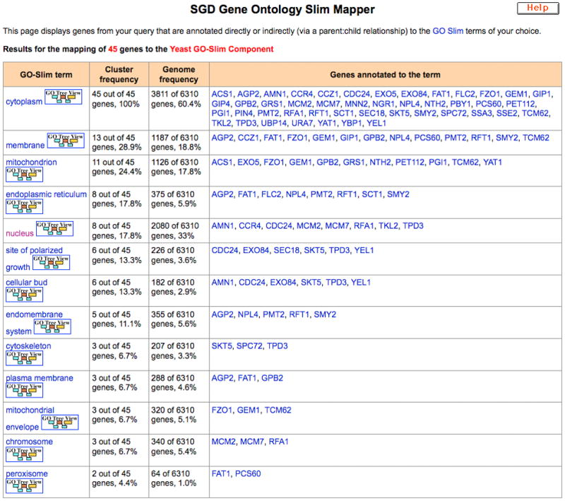
GO Slim Mapper results table for a sample set of 45 genes analyzed for Cellular Component GO Slim annotations. Cluster frequency refers to the frequency with which each term is associated with the genes in the list, either directly, or indirectly through the relationship of that term with more granular terms actually used for annotation. Genome frequency refers to the frequency with which that term is associated with genes in the entire genome, directly or indirectly.

You can also download the results in a tab-delimited file.

You have now mapped each of the genes in your list to a high-level Cellular Component GO term. You may want to further analyze the set of genes in each category, for example, to see the actual granular GO CC terms annotated to each gene. This can be done in YeastMine (see Basic Protocol 3), by creating a list of genes and then using the templates to find the GO terms annotated to the genes. You can also find shared GO terms among the list of genes by looking at the Gene Ontology Enrichment data provided in the widget that appears when you create the list.

Guidelines For Understanding Results

In understanding the output of database searches, it is important to remember the complexity and dynamics of gene-specific information. Gene products may, and often do, have multiple, sometimes seemingly contradictory roles in the cell. Moreover, the information is constantly updated, as new data emerge. Every bit of biological information available in SGD is traceable to the source. Much of it is derived from published, peer-reviewed journal articles. Other sources include protein interaction data from BioGRID, or GO annotations created by mapping associated functions from InterPro protein domains or Swiss-Prot keywords. Regardless of the source, however, different experimental techniques and different algorithms employed in data generation and analysis, in combination with different annotation methods used in data curation, create a complex variety of data types that should not be viewed with the same level of confidence. Manually curated phenotypes or GO annotations based on small-scale research focused on individual genes or proteins often result from the most careful and thorough analysis and therefore reflect the most reliable conclusions, but they may miss a “big picture”. On the other hand, results from large-scale automated studies benefit from a genome-wide scope, uniform experimental conditions and consistent controls, but they may overlook important details about particular genes. Sequence-based predictions provide important clues, but they should be treated as possibilities that await experimental confirmation, rather than established facts. It is therefore the policy of the GO Consortium that any functional predictions can only be based on sequence similarities to experimentally determined gene products. GO annotations are accompanied with evidence codes in order to convey the various degrees of reliability. For instance, annotations inferred from direct assays (IDA) usually provide a direct indication of a biochemical activity, but not always a direct link to a process. On the other hand, annotations inferred from mutant phenotypes (IMP) link to a process, but it may often be an indirect effect. Finally, various experimental techniques have their inherent differences in accuracy, reliability, and resolution that should be considered in evaluating the results. All these caveats should be kept in mind when analyzing the output of a database search. Database searches rarely yield discoveries by themselves; instead, they provide hints that can help in asking the right questions and in designing the experiments aimed at finding the right answers.

Commentary

Background Information

The wealth of knowledge about genetics, biochemistry, and cell biology of the budding yeast Saccharomyces cerevisiae has accumulated over many decades of research. With the release of the S. cerevisiae genome sequence in 1996 (Goffeau et al.,1996), integrating all of the information that used to be scattered among thousands of research papers into a single, widely accessible and easy to use database became necessary. While SGD started as a repository of sequence-based data linked with literature references for S. cerevisiae, over the years it has evolved to become a resource providing access to more types of data (e.g., genetic interactions) and to data mining and analysis tools. SGD serves not only the community of yeast researchers, but also those studying other organisms. S. cerevisiae is currently one of the most thoroughly characterized eukaryotes, due to all its experimental advantages known as “the awesome power of yeast genetics”, but also, in significant part, due to the easy access to all the information that SGD provides. As S. cerevisiae serves as a model for studies in many other organisms, SGD has become a model database for other resources. SGD’s schema, website design and tools have also been used directly as the foundation for at least four other databases: DictyBase (Fey et al., 2009), the Tetrahymena Genome Database (Stover et al, 2006), the Candida Genome Database (Skrzypek et al., 2010), and the Aspergillus Genome Database (Arnaud et al., 2010). SGD maintains collaborations, exchanging ideas and data, with several other resources, including Princeton Protein Orthology Database (P-POD) (Livstone et al., 2011), the BioGRID Interaction Database (Stark et al., 2010), and many other model organism databases.

SGD was designed by biologists, for biologists and those interested in exploring yeast biology. SGD is best understood by a person familiar with the basic concepts of genetics and molecular biology, however experience with S. cerevisiae is typically not assumed. Similarly, users with little or no background in bioinformatics are usually quite able to navigate the SGD pages, retrieve data, and apply SGD’s tools in their own analysis. Most tools are accompanied by extensive help documentation that not only shows how to use them, but also provides detailed explanation of the underlying theory and implemented algorithms. Because the goal is to keep the resource user-friendly, SGD tries to avoid overloading the interfaces with multitudes of options and settings. As a consequence, it is sometimes impossible to meet every user’s needs. In order to make it possible for users to perform analyses of SGD data with their own tools, all information accessible to users via the web interfaces is also available for download in bulk, in a variety of formats, from SGD’s download site at http://downloads.yeastgenome.org/.

The field of yeast research is very active. There are about 100 new publications added to the database each week and the associated information is continually incorporated into SGD. As new data become available, the existing annotations are updated. An overview of what is currently known about the S. cerevisiae genome is available at http://www.yeastgenome.org/cache/genomeSnapshot.html. As new types of data, new analysis methods, and new user interface solutions emerge, SGD re-evaluates and updates its toolbox to better address the needs of the communities we serve.

Critical Parameters and Troubleshooting

Missing or inaccurate representation of data

Because of the large numbers of papers continuing to enter the curation pipeline, SGD has implemented a workflow that ensures we review the newest papers for important information as quickly as possible. In general, papers that contain new data about uncharacterized proteins or new functional data about previously-characterized proteins are deemed the highest priority for in-depth curation. Therefore, data from papers that fall slightly lower on the priority list may take longer to incorporate into the database. If you notice that data are missing, inaccurate, or otherwise out-of-date, we urge you to contact us at: yeast-curator@yeastgenome.org. This address is present at the bottom of most pages in the database.

SGD is dynamic; new data are added continually, and plans for adding new types of data are underway. In particular, we are expanding our collection and display of high-throughput datasets through our GBrowse viewer and YeastMine database. If there are datasets that you would like curators to incorporate, please contact us at the email address above.

Problems using tools

The first place to check regarding questions pertaining to using tools are the Help pages, which are accessible from buttons at the top right of most SGD pages. For help using SPELL, click on the link “About the website” on the right side. The GBrowse Help link is at the top left, within the gold toolbar. Information about using YeastMine can be found by clicking on the “Take a tour” link at the top right of the page.

Problems involving the above tools may be best handled by contacting the SGD curators at the above email address. Curators monitor the email inbox each day and respond to emails the same day they arrive, unless additional work is needed to locate and resolve the problem. In most cases, direct exchange with the curator helps the user better understand how to find the desired information in SGD and helps curators understand how SGD can be improved.

Use of the GO tools requires an understanding of how GO annotations and Evidence Codes are assigned. For more information about GO annotation philosophy and procedures, consult the Documentation section of the GO website: http://www.geneontology.org/GO.contents.doc.shtml

Literature Cited

- Arnaud MB, Chibucos MC, Costanzo MC, Crabtree J, Inglis DO, Lotia A, Orvis J, Shah P, Skrzypek MS, Binkley G, Miyasato SR, Wortman, Sherlock G. The Aspergillus Genome Database, a curated comparative genomics resource for gene, protein and sequence information for the Aspergillus research community. Nucleic Acids Research. 2010 Jan;38(Database issue):D420–427. doi: 10.1093/nar/gkp751. [DOI] [PMC free article] [PubMed] [Google Scholar]
- Cherry JM, Ball C, Weng S, Juvik G, Schmidt R, Adler C, Dunn B, Dwight S, Riles L, Mortimer RK, Botstein D. Nature. 1997;387(6632 Suppl):67–73. Genetic and physical maps of Saccharomyces cerevisiae. [PMC free article] [PubMed] [Google Scholar]
- Costanzo MC, Skrzypek MS, Nash R, Wong E, Binkley G, Engel SR, Hitz B, Hong EL, Cherry JM the Saccharomyces Genome Database Project. New mutant phenotype data curation system in the Saccharomyces Genome Database. Database. 2009 doi: 10.1093/database/bap001. [DOI] [PMC free article] [PubMed] [Google Scholar]
- Degtyarenko K, de Matos P, Ennis M, Hastings J, Zbinden M, McNaught A, Alcántara R, Darsow M, Guedj M, Ashburner M. ChEBI: a database and ontology for chemical entities of biological interest. Nucleic Acids Res. 2008;36:D344–D350. doi: 10.1093/nar/gkm791. [DOI] [PMC free article] [PubMed] [Google Scholar]
- Dwight SS, Balakrishnan R, Christie KR, Costanzo MC, Dolinski K, Engel SR, Feierbach B, Fisk DG, Hirschman J, Hong EL, Issel-Tarver L, Nash RS, Sethuraman A, Starr B, Theesfeld CL, Andrada R, Binkley G, Dong Q, Lane C, Schroeder M, Weng S, Botstein D, Cherry JM. Saccharomyces Genome Database: underlying principles and organisation. Brief Bioinform. 2004;5:9–22. doi: 10.1093/bib/5.1.9. [DOI] [PMC free article] [PubMed] [Google Scholar]
- Engel SR, Balakrishnan R, Binkley G, Christie KR, Costanzo MC, Dwight SS, Fisk DG, Hirschman JE, Hitz BC, Hong EL, Krieger CJ, Livstone MS, Miyasato SR, Nash R, Oughtred R, Park J, Skrzypek MS, Weng S, Wong ED, Dolinski K, Botstein D, Cherry JM. Saccharomyces Genome Database provides mutant phenotype data. Nucleic Acids Res. 2010 Jan;38(Database issue):D433–6. doi: 10.1093/nar/gkp917. [DOI] [PMC free article] [PubMed] [Google Scholar]
- Fey P, Gaudet P, Curk T, Zupan B, Just EM, Basu S, Merchant SN, Bushmanova YA, Shaulsky G, Kibbe WA, Chisholm RL. dictyBase - a Dictyostelium bioinformatics resource update. Nucleic Acids Res. 2009;37(Database issue):D515–19. doi: 10.1093/nar/gkn844. [DOI] [PMC free article] [PubMed] [Google Scholar]
- Goffeau A, Barrell BG, Bussey H, Davis RW, Dujon B, Feldmann H, Galibert F, Hoheisel JD, Jacq C, Johnston M, Louis EJ, Mewes HW, Murakami Y, Philippsen P, Tettelin H, Oliver SG. Life with 6000 genes. Science. 1996;274:546–567. doi: 10.1126/science.274.5287.546. [DOI] [PubMed] [Google Scholar]
- Harris M the Gene Ontology Consortium. The Gene Ontology project in 2008. Nucleic Acids Res. 2008;36:440–444. [Google Scholar]
- Hibbs MA, Hess DC, Myers CL, Huttenhower C, Li K, Troyanskaya OG. Exploring the functional landscape of gene expression: directed search of large microarray compendia. Bioinformatics. 2007;23(20):2692–9. doi: 10.1093/bioinformatics/btm403. [DOI] [PubMed] [Google Scholar]
- Hunter S, Apweiler R, Attwood TK, Bairoch A, Bateman A, Binns D, Bork P, Das U, Daugherty L, Duquenne L, Finn RD, Gough J, Haft D, Hulo N, Kahn D, Kelly E, Laugraud A, Letunic I, Lonsdale D, Lopez R, Madera M, Maslen J, McAnulla C, McDowall J, Mistry J, Mitchell A, Mulder N, Natale D, Orengo C, Quinn AF, Selengut JD, Sigrist CJ, Thimma M, Thomas PD, Valentin F, Wilson D, Wu CH, Yeats C. InterPro: the integrative protein signature database. Nucleic Acids Res. 2009;37(Database Issue):D224–228. doi: 10.1093/nar/gkn785. [DOI] [PMC free article] [PubMed] [Google Scholar]
- Livstone MS, Oughtred R, Heinicke S, Vernot B, Huttenhower C, Durand D, Dolinski K. Inferring protein function from homology using the Princeton Protein Orthology Database (P-POD) Curr Protoc Bioinformatics. 2011 Mar;Chapter 6(Unit 6.11) doi: 10.1002/0471250953.bi0611s33. [DOI] [PMC free article] [PubMed] [Google Scholar]
- Lyne R, Smith R, Rutherford K, Wakeling M, Varley A, Guillier F, Janssens H, Ji W, Mclaren P, North P, Rana D, Riley T, Sullivan J, Watkins X, Woodbridge M, Lilley K, Russell S, Ashburner M, Mizuguchi K, Micklem G. FlyMine: an integrated database for Drosophila and Anopheles genomics. Genome Biol. 2007;8(7):R129. doi: 10.1186/gb-2007-8-7-r129. [DOI] [PMC free article] [PubMed] [Google Scholar]
- MacIsaac KD, Wang T, Gordon DB, Gifford DK, Stormo GD, Fraenkel E. An improved map of conserved regulatory sites for Saccharomyces cerevisiae. BMC Bioinformatics. 2006 Mar;7(7):113. doi: 10.1186/1471-2105-7-113. [DOI] [PMC free article] [PubMed] [Google Scholar]
- Mancera E, Bourgon R, Brozzi A, Huber W, Steinmetz LM. High-resolution mapping of meiotic crossovers and non-crossovers in yeast. Nature. 2008 Jul 24;454(7203):479–85. doi: 10.1038/nature07135. [DOI] [PMC free article] [PubMed] [Google Scholar]
- Skrzypek MS, Arnaud MB, Costanzo MC, Inglis DO, Shah P, Binkley G, Miyasato SR, Sherlock G. New tools at the Candida Genome Database: biochemical pathways and full-text literature search. Nucleic Acids Res. 2010 Jan;38(Database issue):D428–32. doi: 10.1093/nar/gkp836. [DOI] [PMC free article] [PubMed] [Google Scholar]
- Stark C, Su TC, Breitkreutz A, Lourenco P, Dahabieh M, Breitkreutz BJ, Tyers M, Sadowski I. PhosphoGRID: a database of experimentally verified in vivo protein phosphorylation sites from the budding yeast Saccharomyces cerevisiae. Database (Oxford) 2010;2010(2010):bap026. doi: 10.1093/database/bap026. Epub 2010 Jan 28. [DOI] [PMC free article] [PubMed] [Google Scholar]
- Stark C, Breitkreutz BJ, Chatr-Aryamontri A, Boucher L, Oughtred R, Livstone MS, Nixon J, Van Auken K, Wang X, Shi X, Reguly T, Rust JM, Winter A, Dolinski K, Tyers M. The BioGRID Interaction Database: 2011 update. Nucleic Acids Res. 2011 Jan;39(Database issue):D698–704. doi: 10.1093/nar/gkq1116. [DOI] [PMC free article] [PubMed] [Google Scholar]
- Stein LD, Mungall C, Shu S, Caudy M, Mangone M, Day A, Nickerson E, Stajich JE, Harris TW, Arva A, Lewis S. The generic genome browser: a building block for a model organism system database. Genome Res. 2002 Oct;12(10):1599–610. doi: 10.1101/gr.403602. [DOI] [PMC free article] [PubMed] [Google Scholar]
- Steinmetz EJ, Warren CL, Kuehner JN, Panbehi B, Ansari AZ, Brow DA. Genome-wide distribution of yeast RNA polymerase II and its control by Sen1 helicase. Molecular Cell. 2006;24(5):735–746. doi: 10.1016/j.molcel.2006.10.023. [DOI] [PubMed] [Google Scholar]
- Stover NA, Krieger CJ, Binkley G, Dong Q, Fisk DG, Nash R, Sethuraman A, Weng S, Cherry JM. Tetrahymena Genome Database (TGD): a new genomic resource for Tetrahymena thermophila research. Nucleic Acids Res. 2006 Jan 1;34(Database issue):D500–3. doi: 10.1093/nar/gkj054. [DOI] [PMC free article] [PubMed] [Google Scholar]
- Xu Z, Wei W, Gagneur J, Perocchi F, Clauder-Münster S, Camblong J, Guffanti E, Stutz F, Huber W, Steinmetz LM. Bidirectional promoters generate pervasive transcription in yeast. Nature. 2009;457(7232):1033–7. doi: 10.1038/nature07728. [DOI] [PMC free article] [PubMed] [Google Scholar]
- Yassour M, Kaplan T, Fraser HB, Levin JZ, Pfiffner J, Adiconis X, Schroth G, Luo S, Khrebtukova I, Gnirke A, Nusbaum C, Thompson DA, Friedman N, Regev A. Ab initio construction of a eukaryotic transcriptome by massively parallel mRNA sequencing. Proc Natl Acad Sci USA. 2009;106(9):3264–9. doi: 10.1073/pnas.0812841106. [DOI] [PMC free article] [PubMed] [Google Scholar]