

Abstract
This paper explores time heterogeneity in stochastic actor oriented models (SAOM) proposed by Snijders (Sociological Methodology. Blackwell, Boston, pp 361–395, 2001) which are meant to study the evolution of networks. SAOMs model social networks as directed graphs with nodes representing people, organizations, etc., and dichotomous relations representing underlying relationships of friendship, advice, etc. We illustrate several reasons why heterogeneity should be statistically tested and provide a fast, convenient method for assessment and model correction. SAOMs provide a flexible framework for network dynamics which allow a researcher to test selection, influence, behavioral, and structural properties in network data over time. We show how the forward-selecting, score type test proposed by Schweinberger (Chapter 4: Statistical modeling of network panel data: goodness of fit. PhD thesis, University of Groningen 2007) can be employed to quickly assess heterogeneity at almost no additional computational cost. One step estimates are used to assess the magnitude of the heterogeneity. Simulation studies are conducted to support the validity of this approach. The ASSIST dataset (Campbell et al. Lancet 371(9624):1595–1602, 2008) is reanalyzed with the score type test, one step estimators, and a full estimation for illustration. These tools are implemented in the RSiena package, and a brief walkthrough is provided.
Keywords: Stochastic actor oriented models, Longitudinal analysis of network data, Time heterogeneity, Score-type test
1 Introduction
Social networks are relational structures between social actors. They evolve according to potentially complex and dynamic rules. Behavioral variables and static characteristics, the changing network structure itself, and environmental factors may all weigh in on how social networks and their component relationships and actors evolve over time. Understanding this process has become an area of increasing importance among researchers (see, e.g., the three special issues in the Journal of Mathematical Sociology edited by Doreian and Stokman 1996, 2001, 2003, literature on the evolution of friendship networks in Pearson and Michell 2000; Burk et al. 2007, on organizational networks in Borgatti and Foster 2003; Brass et al. 2004).
Increasingly, network data is being collected over time, which gives information about rules for network dynamics that are responsible for changes in network structure. Stochastic actor oriented models (SAOM) proposed by Snijders (2001) and elaborated in Snijders et al. (2010a) provide a flexible framework for statistical modeling of longitudinal network data. Social networks are modeled as digraphs in a Markov chain evolving in continuous time. This continuous time Markov chain (CTMC) changes from one state to the next by modifying a single link at a time. One possible interpretation of this setup is that actors are selected to update an outgoing link according to probabilities resulting from myopic stochastic optimization (see the econometric literature on discrete choice modeling, e.g., Maddala 1983; McFadden 1973). The model is explained in detail in Sect. 2.
Analysis of longitudinal data observed over multiple time periods permits researchers to make inference about the rules governing network evolution; however, the temporal component of panel data may make time heterogeneity an important issue. There are at least two plausible reasons that researchers might neglect time heterogeneity in SAOMs. First, the prospect of including numerous parameters to capture time heterogeneity when such heterogeneity is not a component of the research question is an onerous and time-consuming process. To address this concern, we implement the score-type test of Schweinberger (2007). This allows us to create statistical tests for time heterogeneity without additional computationally intensive estimation runs. Second, it is not well studied in the literature under what circumstances omission of such heterogeneity leads to erroneous conclusions. This paper addresses the potential consequences of omitting time heterogeneity and provides an approach for assessing and accounting for it.
1.1 Motivation for assessing time heterogeneity
The most important consideration in formulating a SAOM is the set of research questions we wish to answer. Let us consider a partitioning of the statistical parameters included in the SAOM, θ = (ψ, ν), where ψ are the parameters of interest and ν are so-called nuisance parameters. Accordingly, ψ is formulated in such a way that it is relevant to the research questions at hand. Keeping in mind that the correctness of inferences about ψ is the principal motivation for considering time heterogeneity, there are at least three important reasons why it should be assessed:
ψ is time heterogeneous: Simulation results given later in the article indicate that incorrectly homogeneous specifications will result in estimates that average over the heterogeneity. Since parameters of interest are intended to answer research questions, detecting heterogeneity in ψ will at least be intrinsically interesting, and sometimes may suggest that some important explanatory covariate has been erroneously omitted. Disruptions in actor behavior may be crucial in certain settings. For example, drawing inference on time heterogeneity will help with understanding periods of disrupted behavior in illicit networks, cooperation networks for natural disasters, and planned restructuring of organizations.
Undetected heterogeneity may lead to bias in other parameters: It is currently unknown in the literature whether time heterogeneity in ν can have serious consequences for inferences about ψ. Accordingly, it is prudent to formulate models which take into consideration time heterogeneity in all of the parameters in the model.
Asymptotic degeneracy of the model: SAOMs are based on a right-continuous process on the set of all possible networks, and the unique, limiting distribution of a continuous-time Markov process as t → ∞ under time-homogeneous parameterizations may be near-degenerate in the sense of placing much—sometimes almost all—probability mass on a small number of graphs which do not resemble real-world networks. Strauss (1986), Snijders (2002), Handcock (2003) show that exponential random graph models can be near-degenerate, and the same may hold for SAOMs if time runs on infinitely long (although in practice, time usually is limited). While the limiting distribution in itself is rarely of interest, this suggests that statistical inference can be affected when the amount of change between consecutive observations is large.
Since it is not possible to determine a priori that these cases do not apply, the study of time heterogeneity is motivated anywhere it could exist—namely whenever a dataset contains more than one time period.
We proceed with a review on SAOM in Sect. 2. We then review the score type test proposed by Schweinberger (2007) and develop a specific test for time heterogeneity in Sect. 3. A simulation study follows to explore the validity of the score type approach for detecting time heterogeneity in Sect. 4. The paper culminates with a case study on a dataset collected by Audrey et al. (2004) with suspected time heterogeneity in Sect. 5. This study also provides an opportunity to demonstrate functionality implementing the aforementioned score type test now available in the RSiena package (see Ripley and Snijders 2009) in Sect. 5.1.
2 Stochastic actor oriented models (SAOM)
A social network composed of n actors is modeled as a directed graph (digraph), represented by an adjacency matrix (xi j)n×n, where xi j = 1 if actor i is tied to actor j, xi j = 0 if i is not tied to j, and xii = 0 for all i (self ties are not permitted). It is assumed here that the social network evolves in continuous time over an interval
 ⊂ ℝ1 according to a Markov process. Accordingly, the digraph x(t) models the state of social relationships at time t ∈
. Changes to the network called updates, occur at discrete time points defining the set
⊂ ℝ1 according to a Markov process. Accordingly, the digraph x(t) models the state of social relationships at time t ∈
. Changes to the network called updates, occur at discrete time points defining the set
 ⊂
. Elements of the set are denoted La with consecutive natural number indices a so that L1 < L2 < ··· <
⊂
. Elements of the set are denoted La with consecutive natural number indices a so that L1 < L2 < ··· <
 , where the notation |.| is used to denote the number of elements in a set. The network is observed at discrete time points called observations defining the set
 with elements Ma indexed similarly with consecutive natural number indices a so that M1 < M2 < ··· <
 . Define a set of periods with elements Wa ∈
 each representing the continuous time interval between two consecutive observations Ma and Ma+1:
By definition, |
| = |
| − 1. When
=
, we have full information on the network updates over the interval
. We use upper case to denote random variables (e.g. X, M, L).
There is a variety of models proposed in the literature for longitudinally observed social networks. In this paper, we consider the approach proposed by Snijders (2001), the stochastic actor oriented model (SAOM). Here, the stochastic process {X (t): t ∈
} with digraphs as outcomes is modeled as a Markov process so that for any time ta ∈
, the conditional distribution for the future {X (t): t > ta} given the past {X (t): t ≤ ta} depends only on X (ta).
From the general theory of continuous-time Markov chains (Norris 1997) follows the existence of the intensity matrix that describes the rate at which X (t) = x tends to transition into X̃(t + dt) = x̃ as dt → 0:
| (1) |
where x̃ ∈
 . The SAOM supposes that a digraph update consists of exactly one tie variable change. Such a change is referred to as a ministep. This property can be expressed as
| (2) |
where abs(.) denotes the absolute value. Therefore we can use the notation
| (3) |
SAOMs consider two principal concepts in constructing the intensity matrix: how often actors update their tie variables and what motivates their choice of which tie variable to update. This is expressed by the formulation
| (4) |
The interpretation is that actor i gets opportunities to make an update in her/his outgoing tie at a rate of λi (x) (which might, but does not need to, depend on the current network); if such an opportunity occurs, the probability that i selects xi j as the tie variable to change is given by pi j (x). The actors are not required to make a change when an opportunity occurs, which is reflected by the requirement Σ j pi j (x) ≤ 1, without the need for this to be equal to 1. The probabilities pi j (x) are dependent on the so-called evaluation function, as described below.
2.1 Rate function
The rate function describes the rate at which an actor i updates tie variables. Waiting times between opportunities for actor i to make an update to the digraph are exponentially distributed with rate parameter λi (x), and it follows that waiting times between any two opportunities for updates across all actors are exponentially distributed with rate parameter
| (5) |
It is possible to specify any number of functional forms for λi (x) as long as λi (x) is positive, to include combinations of actor-level covariates and structural properties of the current state of the network x; however, in many applications, rate functions are modeled as constant terms.
2.2 Evaluation function
Once an actor i is selected for an update, the actor must select a tie variable xi j to change. Define x(i ⇝ j) ∈
as the digraph resulting from actor i modifying his tie variable with j during a given time period t so that xi j (i ⇝ j) = 1 − xi j, and formally define x(i ⇝ i) = x.
The SAOM assumes that the probabilities pi j (x) depend on the evaluation function that gives an evaluation of the attraction toward each possible next state of the network, denoted here by fi j (x). This attraction is conveniently modeled as a linear combination of the relevant features of each potential change i ⇝ j:
| (6) |
where si is a vector-valued function containing structural features of the digraph as seen from the point of view of actor i, and β is a statistical parameter. Snijders (2001), following the the econometric literature on discrete choice (see e.g., Maddala 1983; McFadden 1973), models the choice of i ⇝ j as a myopic, stochastic optimization of a conditional logit. This amounts to choosing the greatest value fi j (x) + εi j, where εi j is a Gumbel distributed error term. This leads to the conditional choice probabilities pi j (x) that actor i chooses to change tie variable i ⇝ j given the current digraph x:
| (7) |
In accordance with the formal definition x(i ⇝ i) = x, the choice j = i is interpreted as keeping the current digraph as it is, without making a change. For a thorough menu of what kinds of statistics si are appropriate for actor oriented models (see Ripley and Snijders 2009; Snijders et al. 2010a). We will present here three fundamental structural statistics which are used throughout this paper: outdegree (density), reciprocity, and transitive triplet effects:
- Outdegree (density) effect, defined by the number of outgoing ties that an actor has:
(8) - Reciprocity effect, defined by the number of outgoing ties that are matched (or reciprocated) by a corresponding incoming tie:
(9) -
Transitive Triplet, defined by the number of patterns matching the following Fig. 1:
(10) These three features are considered fundamental to social network dynamics, but more features may also be formulated. One possibility is to include exogenous actor-level covariates c ∈ ℝn. In Sect. 5, a simple covariate statistic is used:
-
Same covariate defined by the number of actors j tied to actor i sharing the same value of c:
(11) where we define the covariate equivalence function(12) -
Covariate similarity defined by the number of actors j tied to actor i having a similar value of c:
(13) where we define the covariate similarity function(14)
Fig. 1.
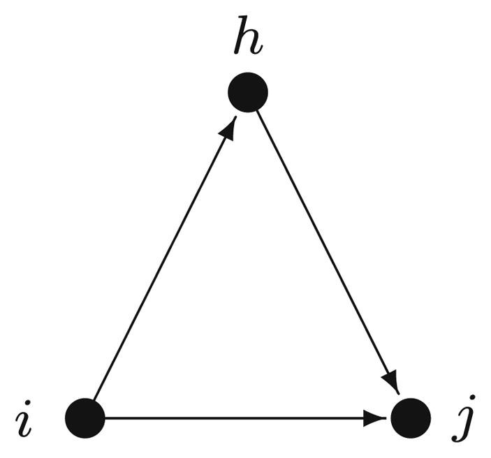
The transitive triplet
See also Snijders (2001), Snijders et al. (2007), Snijders (2009), Snijders et al. (2010a) for thorough developments of possible statistics and extensions to models which consider the coevolution of network and endogenous behavioral characteristics.
2.3 Estimation
A key feature of (7) is the convenient form of its log odds ratios between any two potential next networks x(i ⇝ j) and x(i ⇝ k):
| (15) |
This is the characteristically simple property that makes estimation in classical discrete choices quite straightforward (see e.g., Greene 2007), and is also the basis for the SAOM. If the network updates
are all observed so that we have full information (i.e.
=
), and if the rate parameters are independent of the parameters of the objective function (as is usually the case), a convenient partial likelihood is available for the statistical parameters of the objective function. We use the notation x(a) = x(Ma) = x(La) for the ath network observed in the dataset.
Define a vector of binary variables d such that
| (16) |
which denotes whether actor i selected variable to update. Note that for all a. The partial log likelihood for the objective function parameters is
| (17) |
Under regularity conditions, a solution β̂ML to
where
is a maximum likelihood estimate for β.
Unfortunately, complete information on each network update is extremely rare, and a likelihood function as in (17) is not readily available if some transitions are unobserved. Even when tie creation is observed in continuous time, it is not often that observations concerning termination of ties are also available. It is far more often the case that the data observed will be in the form of panel data, where typically |
| ≪ |
|. Accordingly, the method of moments as proposed by Snijders (2001) can be used as an alternative method for obtaining reasonable estimates. Consider the estimating function
| (18) |
which is simply the sum of deviations between the expected value of the statistics for the random (simulated) networks and the observed networks; zn simply means all of the available data, and θ is a vector of parameters for the objective and rate functions described earlier. u(x) is a function that corresponds to appropriately chosen statistics calculated from the digraph for the parameters θ (based on the statistics in 2.2). It is helpful to note that Eθ {gn(θ; zn)} does not depend on zn, so it is not random. The method of moments involves finding the moment estimate θ̂ solving the moment equation
| (19) |
The specific details of fitting moment estimates are rather involved, and entail simulating networks X(a) many times to achieve a reliable result for the expectation in (19).1 This simulation is very straightforward. Take an initial network x(l1) and proceed as follows for each update la ∈
:
Set la = la−1 + Expon(λ+)
Select actor i with probability .
Select actor j with probability pi j (la−1).
If i ≠ j, set xi j (la) = 1 − xi j (la−1).
Repeat until some specified conditions (e.g. number of updates |
| or some holding time (
 − la) is exceeded) are satisfied.
See Snijders (2001), Snijders et al. (2010a) for guidelines on the selection of appropriate statistics for u(X (t)) and information on how to estimate the root of gn(zn, θ), and Schweinberger and Snijders (2007) for the estimation of the derivative matrix, covariance matrix, and standard errors.
2.4 Estimator (β̂) properties
The properties of parameter estimates β̂ in SAOM have yet to receive a great deal of attention in the literature. Understanding the conditions under which desirable estimator properties (i.e. approximate unbiasedness, consistency, and efficiency) exist is an important feature for non-experimental studies with social networks, since erroneous conclusions could be drawn from the results. In the classical discrete choice literature, early attempts at uncovering the relationship between omitted variables and biased estimates in multinomial/conditional logit models include Amemiya and Nold (1975), Lee (1982), Ruud (1983), Yatchew and Griliches (1985), Wooldridge (2002), but fail to uncover an analytical form for bias in general. It is desirable to investigate similar properties for the estimators of SAOM, especially the form of any omitted variable biases. Unfortunately, closed forms for estimates of β and of var(β̂) are unavailable for all but the most simple SAOMs (see Snijders 2005; Van De Bunt et al. 1999). Compounded with the lack of analytical results for even classical discrete choice models, straightforward analysis of SAOM estimates is very difficult. Accordingly, we utilize simulation study to uncover some basic results on bias and efficiency under model misspecifications in Sect. 4.
3 Assessing time heterogeneity with the score type test
Consider a SAOM formulated as in (6) with some set of effects
 included. We initially assume that β does not vary over time, yielding a restricted model. Our data contains |
| ≪ |
| observations, so we estimate the restricted model by the method of moments mentioned in Sect. 2.3. For reasons introduced in Sect. 1.1, we wish to test whether the restricted model is misspecified with respect to time heterogeneity. An unrestricted model which allows for time heterogeneity in all of the effects is considered as a modification of (6):
included. We initially assume that β does not vary over time, yielding a restricted model. Our data contains |
| ≪ |
| observations, so we estimate the restricted model by the method of moments mentioned in Sect. 2.3. For reasons introduced in Sect. 1.1, we wish to test whether the restricted model is misspecified with respect to time heterogeneity. An unrestricted model which allows for time heterogeneity in all of the effects is considered as a modification of (6):
| (20) |
where
is called the time dummy interacted effect parameter for effect k and period a. Define also the vectors
and δ = (δ1, …,
 ). Equation (20) applies for updates occurring during the period Wa. By convention,
for all k ∈
so that the first period is called the base period; therefore, the vector of time dummy interacted effect parameters δ has length (|
| − 1)|
|.2 One way to formulate the testing problem of assessing time heterogeneity is the following omnibus test:
). Equation (20) applies for updates occurring during the period Wa. By convention,
for all k ∈
so that the first period is called the base period; therefore, the vector of time dummy interacted effect parameters δ has length (|
| − 1)|
|.2 One way to formulate the testing problem of assessing time heterogeneity is the following omnibus test:
| (21) |
If we consider the unrestricted model parameters for (20) as θ1 = (β, δ), and the restricted model parameters for (6) as θ0 = (β, 0), there are three broad routes in likelihood-based inference for testing H0: θ0 = 0: the likelihood ratio test, the Wald test, and the score test. Each of these routes requires different estimates to be calculated.
A likelihood ratio test statistic would take the form
| (22) |
To construct ηL, we estimate the unrestricted model parameters θ̂1, the restricted model parameters θ̂0, and evaluate the likelihoods for the restricted and unrestricted models. There is a major difficulty with using this approach for a SAOM: when
≠
, the likelihood for SAOM parameters is not available in closed form, although Snijders et al. (2010b) consider a maximum likelihood estimation approach for SAOM using data augmentation methods. As we will see, pursuing the likelihood ratio testing route will be the most computationally expensive among those asymptotic approaches considered here. Note three important features of evaluating ηL: (1) both the restricted and unrestricted model parameters must be estimated, (2) we must evaluate the likelihood functions at these estimates, and (3) finding maximum likelihood estimates is more computationally expensive than finding method of moments estimates.
We might also consider a Wald test statistic of the form
| (23) |
where i(θ̂1) is the expected (Fisher) information matrix and [i−1 (θ̂1)]δδ refers to the block corresponding to δ.3 Unlike ηL, the Wald statistic ηW does not require estimation of θ0; however, since we must know θ̂1, we still must estimate the unrestricted model.
The score test statistic is defined by
| (24) |
where we only require the expected information matrix i(θ̂0) and the score function U(θ̂0).4 An advantage here is that the score test statistic ηU only requires a score function and the expected information matrix, and these ingredients do not require estimates for the unrestricted model. For a review of the classic asymptotic approaches to approximate inference presented above (see e.g. Cox and Hinkley 1974; Cox 2006; Lehmann and Romano 2005).
These three tests are classical tests for inference based on maximum likelihood estimation. However, for the SAOM, the maximum likelihood estimators recently developed by Snijders et al. (2010b) are computationally so demanding that in practice the more easily calculated method of moment estimators of Snijders (2001) and Schweinberger and Snijders (2007) are used. This type of inference is also called inference based on estimating functions or M-estimation. For inference using the method of moments, generalizations of the Wald test and score test are available, as proposed for the score test by Rao and Poti (1946), Rao (1948), Neyman (1959), Basawa (1985, 1991), and reviewed by Rippon and Rayner (2010).
Because δ has length (|
| − 1)|
|, estimating it with method of moments is infeasible for even modest numbers of periods and effects. For example, given a modestly sized model containing 8 effects and a dataset with 5 periods, 40 parameters must be estimated (8 base effects β and 32 time dummy interaction effect parameters δ). Estimations of this size can begin to become unstable and computationally costly (particularly with larger numbers of actors, e.g. n > 150). We therefore take the forward-selecting approach to model selection, where we start by estimating only the base effects and add time dummy interaction effects only when there is empirical evidence or when there is some theoretical reason. The score-type test manifests naturally in such an approach. For the SAOM, it was proposed by Snijders (2001) to test parameters by a test which can be regarded as the analogue of the Wald test for estimates obtained by the method of moments. The generalization of the score test based on moment estimators for the SAOM was elaborated by Schweinberger (2007) following methods proposed by Basawa (1985, 1991). This requires analogues of U() and i() as used in (24), which are derived in the following way.
By Δ(θ) we denote the Jacobian,
We partition the estimating function gn(θ̂0; zn), the covariance matrix of the estimating functions Σ(θ̂0), and the Jacobian Δ(θ̂0),
| (25) |
| (26) |
| (27) |
so that subscript 1 corresponds to the restricted model and subscript 2 corresponds to the additional terms of the unrestricted model (i.e. the time dummy interacted effect parameters). We orthogonalize the moment function g2(θ̂0; zn) of the nuisance parameters in g1(θ̂0; zn) to yield:
| (28) |
where
We now calculate Ξ (θ̂0), the asymptotic covariance matrix for bn(θ̂0; zn):
| (29) |
giving rise to the test statistic
| (30) |
with an asymptotic χ2 distribution with degrees of freedom equal to the number of terms in bn(θ̂0; Zn). We will make use of this test statistic in assessing null hypotheses for time dummy interacted effect parameters.
So long as gn(θ̂0; zn) is differentiable at θ̂0, the same Taylor-series approximation used to calculate the covariance matrix Ξ(θ̂0) (the delta method) can be manipulated to solve for a one-step estimator, which is a “quick and dirty” estimator that does not require the use of likelihood or moment equations (see e.g., Schweinberger (2007)):
| (31) |
We will test the effectiveness of the one-step estimator thoroughly in Sect. 4.
After SAOM parameters are estimated, we typically simulate the network evolution according to the estimated parameters thousands of times so that we can estimate standard errors. Using these simulations, we estimate the expected values for the estimating functions in (18) using the simulated and observed statistics. Conveniently, the simulations are conducted independently for each period in
, so that we also have the estimating functions in (18) for the time dummy interacted effects.
3.1 Guidelines on selecting a decision procedure and constructing test statistics
There is an array of hypothesis tests which are available from these ingredients, which permit a number of procedural approaches to assessing time heterogeneity and ultimately refining the model. We present an iterative, forward-selecting procedure below. This decision procedure is informal, but in the absence of a universally superior rule, it is a reasonable approach to refining model selection. We also note here that outdegree effects will be given a privileged position in the selection of time dummy terms. The reason is that the outdegree is highly correlated with most other effects.
The decision procedure proceeds as follows:
Estimate the parameters of some arbitrary restricted model using the method of moments. We refer to this model as restricted with respect to the set of time dummy interacted effect parameters, because many or all of these are assumed to be zero in the model. Denote by δ† the vector of time dummy interacted parameters which are zero in the restricted model and which the researcher would like to test.
-
Test the composite hypothesis
(32) Evaluate bn(zn, θ̂0) and Ξ by including all δ† terms in those ingredients of (25), (26), and (27) with subscript 2. Follow the procedure outlined above for orthogonalizing the testing function (28) of the nuisance parameters θ† and estimating Ξ in (29). Construct the test statistic(33) which is asymptotically distributed χ2 with degrees of freedom equal to the number of elements in δ†. If we fail to reject , stop.
-
If is rejected, select one to include in the model by considering two quantities. First, evaluate
(34) for each a, k combination. Each is a test statistic for(35) and is distributed standard normal. In interpreting this array of test results, one should take into account that each test is directed at the overall null hypothesis , and it is possible that the test based on yields a significant result not because of itself, but because some other is non-zero.
Evaluate the one step estimators θ̂* to see which has the greatest magnitude.
Select one using the hypothesis test results and the one step estimators for inclusion. Because of what was mentioned in Step 3, the results for all k, a should be considered simultaneously, and substantive background knowledge and the researchers judgment will be important in making this choice. We highly recommend that outdegree heterogeneity is given a privileged position in this selection.
Set , i.e. remove from the vector δ†.
Set , i.e. add to the restricted model.
Return to Step 1.
This model selection process is ended when we fail to reject . An advantage to this approach is that all of the evidence for time heterogeneity is assessed near the current estimate , and we iteratively update it in an attempt to keep the local approximations valid. A disadvantage is that we must make one successively more computationally costly estimation for each time dummy term that is included.
4 Simulation study
The simulation study is conducted to achieve three purposes: (1) to better understand the properties of β̂ and its standard errors when a model is improperly specified with respect to time heterogeneity, (2) to investigate the validity and relative efficiency of one step estimates as a tool for assessing time heterogeneity, and (3) to analyze the type I and II errors of the various available hypothesis tests from the score-type approach. The same simulation setup is used to address each of these research questions. A |
| = 2-period dynamic network of n = 50 actors is generated with parameters for outdegree β11 = −1.25, reciprocity β12 = 2, and transitivity β13 = 0.25 at period w1, and rate parameters λ = 1.5 for both periods, values which are in line with many observed datasets (see e.g., Snijders 2001; Snijders et al. 2010a).
We create a basis for comparison by simulating a base model SAOM with no time heterogeneity using the aforementioned setup. The parameters for the restricted specification, which correspond to the outdegree, reciprocity, and transitive triplets effects (i.e. no time dummy interactions), are estimated in a time homogeneous restricted estimation. The series of score-type tests and one step estimators described in Sect. 3 are then carried out using the results from the restricted estimation.
Next, a series of nine perturbed models are considered. At period w2, some level of perturbation is introduced to one of the effects during generation (there are three levels). Since the restricted specification is improper for a perturbed model, we can compare the results from the base model by conducting a restricted estimation to see how the improperly specified parameter estimates behave. The score-type tests and one step estimators are obtained from the ingredients in the restricted estimation results. Finally, a properly specified set of parameters (i.e. the unrestricted specification) is estimated in an unrestricted estimation so that we can compare the relative efficiency of the one step estimate with the traditional method of moments estimate.5 Using the results from these simulations, we treat each research purpose in turn:
4.1 Validity of the method of moments estimators
We investigate the performance of these estimators here by the Monte Carlo simulations detailed above. Let [β̂k]i be the ith from a set of N estimates from independently simulated data with identical effect parameter vectors. We use a one sample t test to investigate bias. Assuming that is asymptotically distributed , we test H0: bias = 0 by evaluating the t statistic
for each parameter. Table 1 contains the results of this hypothesis test: outdegree, transitive triplet, and rate parameters indicate a statistically significant bias. However, the magnitude of this bias is very small and of no concern; the method of moments estimators for properly specified SAOMs are approximately unbiased and have appropriate standard errors.
Table 1.
This table provides a comparison of observed and population parameters for a properly specified SAOM from N = 1,000 independent Monte Carlo simulations with an independent, one sample t test
| Effect | Bias | μ̂k | σ̂k | ||
|---|---|---|---|---|---|
| Outdegree (density) | 0.012 | −1.24 | 0.163 | 2.24 | |
| Reciprocity | 0.005 | 2.00 | 0.250 | 0.57 | |
| Transitive triplets | −0.013 | 0.24 | 0.105 | −3.86 | |
| Rate 1 | 0.010 | 1.51 | 0.213 | 1.48 | |
| Rate 2 | 0.019 | 1.52 | 0.210 | 2.83 |
Restricted estimations of the perturbed models indicate that restricted estimators for unperturbed effects (e.g. the estimated parameter for reciprocity effect in a restricted specification when outdegree is perturbed) are also approximately unbiased with appropriate standard errors. Further, the distributions of the method of moments estimates are almost identical to the restricted estimates for the unperturbed effects. Figures 2 and 3 illustrate these findings (refer to the black, dotted lines centered on the vertical reference line). The figures for outdegree effect are similar, but omitted for brevity.
Fig. 2.

Omitting reciprocity time heterogeneity: density plots illustrating approximate unbiasedness of estimates for time homogeneous parameters in the presence of simulated reciprocity time heterogeneity. The two solid curves correspond to the distributions of the one step estimates β̂* and β̂* +δ̂* (i.e. the base period parameter—in gray—and the base period plus time heterogeneity term—in black, slightly broader than the base period). The two (indistinguishable) dotted curves correspond to the method of moments estimates for β under the unrestricted and restricted models (i.e. estimated with and without the time heterogeneity parameter included for reciprocity). The vertical reference lines correspond with the population generating quantities for each effect parameter
Fig. 3.

Omitting transitive triplets time heterogeneity: Density plots illustrating approximate unbiasedness of estimates for time homogeneous parameters in the presence of simulated transitive triplets time heterogeneity. The two solid curves correspond to the distributions of the one step estimates β̂* and β̂* + δ̂* (i.e. the base period parameter—in gray—and the base period plus time heterogeneity term—in black, slightly broader than the base period). The two (indistinguishable) dotted curves correspond to the method of moments estimates for β under the unrestricted and restricted models (i.e. estimated with and without the time heterogeneity parameter included for transitive triplets). The vertical reference lines correspond with the population generating quantities for each effect parameter
This finding is surprising, as we might expect some difficulty in estimating parameters and standard errors in a misspecified model. This robustness might be due in part to the rather simple specification of the models used in the study, but it is an encouraging indication that method of moments estimation is resilient to time heterogeneity when a model is improperly specified. Along the same lines, we find that the expected value for the restricted estimates of perturbed effect parameters is wβ1k + (1 − w)β2k where w ≈ 0.5—which may be due to the constant rate parameters across periods. Figures 4 and 5 illustrate these findings; the black density plots in the left column correspond to the restricted estimates and lie centered between β1k and β2k. Again, the figures for outdegree effect are similar, but omitted for brevity.
Fig. 4.

Performance of the reciprocity effect parameter one step estimators: this figure plots parameter estimates in the left column. For these figures, the fine, black density plot (the tallest among the plots) represents the restricted estimate. To either side of this restricted parameter density plot are the period-wise estimates for the unrestricted model. The dotted density plot represents the one step estimates, and the bold density plots represent the method of moments estimators. The true period-wise values are given by vertical reference lines. On the right, estimates of the parameter estimate variances are shown. The black plots represent the variance estimators from the restricted estimation and the gray plot represents the variance of the unrestricted estimates. Vertical lines represent the sample variances
Fig. 5.

Performance of the transitive triplet effect parameter one step estimators: this figure plots parameter estimates in the left column. For these figures, the fine, black density plot (the tallest among the plots) represents the restricted estimate. To either side of this restricted parameter density plot are the period-wise estimates for the unrestricted model. The dotted density plot represents the one step estimates, and the bold density plots represent the method of moments estimators. The true period-wise values are given by vertical reference lines. On the right, estimates of the parameter estimate variances are shown. The black plots represent the variance estimators from the restricted estimation and the gray plot represents the variance of the unrestricted estimates. Vertical lines represent the sample variances
Also evident from these figures is the approximate unbiasedness of the method of moments estimates of effect parameters with simulated time heterogeneity as expected from the base model results (i.e. proper specifications correspond with approximately unbiased parameter estimates).
4.2 Approximate validity and relative efficiency of one step estimates
Restricted estimations of the perturbed models indicate that one step estimates using the ingredients from restricted estimators for unperturbed effects (e.g. the one step estimates for reciprocity effect and its time dummy interaction in a restricted specification when outdegree is perturbed) are approximately unbiased. Referring to the dotted density plots in Figs. 2 and 3 the reader may visually confirm this finding. The one step estimators for time dummy interacted effect parameters are, however, less effective at detecting time homogeneity than method of moments estimates as evidenced by their relatively flat density plots. In other words, when time heterogeneity does not exist, one step estimates will have wider dispersion than method of moments estimates, illustrating their “quick and dirty” nature.
The one step estimates for the perturbed effects (i.e. in the case with time heterogeneity in the simulated effect) are likewise approximately unbiased. Surprisingly, the one step estimates for perturbed reciprocity and transitive triplet effect parameters are at least as efficient as their method of moments counterparts. The dotted density plots of Figs. 4 and 5 illustrate these results. The outdegree results are mixed; nonetheless, the estimators perform well on balance. Figures of outdegree results are omitted for brevity.
In short, the one step estimators are approximately valid in that they are unbiased (i.e. their expected values correspond to the true model under both time heterogeneous and homogeneous parameterizations). This simulation study indicates that the one step estimators are less efficient under homogeneous conditions, since method of moments estimates have less variance. When there is time heterogeneity in the effects, however, one step estimates perform as well as their method of moments counterparts. To further synthesize the relationship between the one step and method of moments estimates, we report Pearson correlation coefficients in Table 2. There is a clear, positive correlation between the two estimates, which further supports the approximate validity of the one step estimates as a tool to detect time heterogeneity.
Table 2.
Correlations among the one step estimates and the method of moments estimates: this table presents the Pearson correlation coefficient between the one step estimates and the method of moments estimates for the unrestricted model parameters for each treatment group indicated by row title
| Effectk | βk | ||
|---|---|---|---|
| Outdegree (+0.3) | 0.79 | 0.91 | |
| Outdegree (+0.6) | 0.87 | 0.90 | |
| Outdegree (+0.9) | 0.85 | 0.82 | |
| Reciprocity (+0.25) | 0.92 | 0.96 | |
| Reciprocity (+0.5) | 0.93 | 0.96 | |
| Reciprocity (+0.75) | 0.94 | 0.97 | |
| Transitive triplets (+0.1) | 0.85 | 0.93 | |
| Transitive triplets (+0.2) | 0.85 | 0.93 | |
| Transitive triplets (+0.3) | 0.67 | 0.94 |
The level of simulated time heterogeneity is provided in parenthesis
Correlations close to one indicate that the one step estimates and the method of moments estimates tend to agree on the direction of the heterogeneity
4.3 Effectiveness of the score-type test
There are two important properties of the score-type test which we consider here: type I error and power. The approach for evaluating the type I error is to first validate that the distributions used to evaluate the hypotheses of Sect. 3 are valid. We conduct the score-type tests for both joint significance and individual significance using χ2 distributions with the appropriate d.f., yielding p values. These p values are assembled into receiver operating characteristic (ROC) curves, which represent the probability of rejection of the test as a function of its nominal significance level (i.e. α or type I error level). These should resemble the cumulative density function for a uniform distribution Unif (0, 1) when the null hypothesis is true (i.e. there is time homogeneity in the effect parameters).6 Figure 6 illustrates that the score-type test meets this criterion.
Fig. 6.

Charts for statistical tests: receiver operating characteristic (ROC) curves. Dotted gray curves correspond to individual tests for the effect indicated by the plot’s title when is true. For three levels of time heterogeneity, the solid gray and solid black curves plot the results of the individual and joint tests, respectively. Uniformly more powerful curves correspond with greater levels of time heterogeneity
When H0 is false, the ROC curves indicate the power on the vertical axis for varying type I error rates on the horizontal axis. It is desired that power is as high as possible for all type I error rates.
While it is straightforward to validate the type I error indicated by the score-type test, there is no objective basis over which to evaluate the power of these tests. Nonetheless, there are some key features available from the results. As expected, greater heterogeneity in the effect parameter leads to greater power in detecting the heterogeneity. Additionally, these results enrich the previous findings by illustrating that perturbations of {+0.6, +0.9} on the outdegree effect parameter correspond to the most powerful of the score-type tests (while {+0.3} is the least powerful).
The score tests of the different parameters will be correlated to an a priori unknown extent. When computing test statistics for individual parameters , a very rough approximation is possible based on the covariance matrix Ξ in (29): the scores of all other are included in g1(zn, θ̂0) of (25) in addition to the parameters θ† which have been estimated by the method of moments. This approximation is valid only in the close vicinity of the overall null hypothesis , and it may not hold for parameter values away from this null hypothesis. Table 3 shows that for the case of various levels of simulated outdegree time heterogeneity, the individual test statistics are strongly correlated.
Table 3.
Pearson correlation coefficients between t statistics for individual time heterogeneity parameter significance tests in the presence of simulated outdegree time heterogeneity
| ta | tb | cor(ta, tb) | ||
|---|---|---|---|---|
| Outdegree (+0.0) | Reciprocity | 0.06 | 0.46 | |
| Outdegree (+0.3) | Reciprocity | 0.05 | 0.43 | |
| Outdegree (+0.6) | Reciprocity | 0.05 | 0.44 | |
| Outdegree (+0.9) | Reciprocity | 0.06 | 0.49 | |
| Outdegree (+0.0) | Transitive triplets | −0.06 | 0.64 | |
| Outdegree (+0.3) | Transitive triplets | −0.10 | 0.62 | |
| Outdegree (+0.6) | Transitive triplets | −0.09 | 0.69 | |
| Outdegree (+0.9) | Transitive triplets | −0.13 | 0.67 |
The magnitude of the heterogeneity is given in parenthesis.
Test statistics treated with approximate orthogonalization based on Ξ in (29) are denoted with a superscript ⊥
The practical significance of this result is the following: when is false, all of the individual tests have a tendency to show evidence for time heterogeneity—even those effect parameters which are time homogeneous. This complicates procedures such as the one given in Sect. 3.1, since the selection of how to iteratively update θ† is based in part on these individual test statistics.7 Using the approximate orthogonalization above, dependence may be substantially reduced in some limited situations. Table 3 shows that both reciprocity and transitive triplets time heterogeneity parameters are only weakly correlated after performing the approximate orthogonalization. The rough approximation may be valid in the present circumstances due to the sparsity of effect parameters and to the small magnitude of overall time heterogeneity in the parameters; however, the validity of this procedure needs further investigation before it can be applied generally.
5 Application: Bristol and Cardiff’s ASSIST data
Campbell et al. (2008) conducted a study funded by the UK Medical Research Council which involved peer-nominated students aged 12–14. These individuals underwent intensive training on how to discourage their peers from smoking. The complete data-set contains data on over 10,000 students.8 Smoking behavior, friendship nomination, sex, age, parental smoking habits, family affluence, and nominal information on classroom membership are all features of the dataset. There are a number of interesting research questions supported by this study. In the following analysis, we wish to find whether an ego’s smoking behavior affects nomination of alters on the basis of the alter’s smoking behavior (i.e. selection).9
Because the dataset was collected over a three year period where adolescents are likely to modify social behavior, any assumptions of time homogeneity are suspect. Additionally, Steglich et al. (2010) notes that the ASSIST dataset contains substantial time heterogeneity in some important parameters of interest. Ultimately, they chose to mitigate the heterogeneity by estimating period 1 → 2 separately from 2 → 3, effectively dummying all of the effect parameters.
Due to potential convergence issues in estimation with models containing large numbers of parameters (and for illustrative purposes), we first specify a restricted model with period-wise independence for the rate parameters only. We specify as network effects the following: basic first and second order structural dependencies (outdegree, reciprocity, and transitive triplets), smoking similarity, same form (a control for the classroom to which the student is assigned), age similarity, and same sex effects (refer to Sect. 2.2 for an explanation of these effects).
We then estimated the restricted model using RSiena (Ripley and Snijders 2009). All of the effects achieved good convergence, as indicated by near-zero convergence t statistics. Results from this estimation are contained in Table 4. The rest of the terms support our intuition: age, smoking, sex, and classroom similarity increase the probability that an actor chooses an alter. Basic first and second order dependencies in reciprocity and transitive triplets also make links more attractive.
Table 4.
Estimates for a restricted SAOM model of the Cardiff ASSIST data (Campbell et al. 2008)
| Effect name | θ̂ | se(θ̂) | t. conv. | θ̂* | p value |
|---|---|---|---|---|---|
| Rate (1) | 16.762 | 1.290 | – | – | – |
| Rate (2) | 10.834 | 0.681 | – | – | – |
| Outdegree | −2.892 | 0.029 | −0.034 | −2.910 | – |
| (2) | – | – | – | 0.042 | 0.467 |
| Reciprocity | 1.958 | 0.065 | 0 | 1.935 | – |
| (2) | – | – | – | 0.056 | 0.673 |
| Transitive triplets | 0.415 | 0.015 | −0.025 | 0.457 | – |
| (2) | – | – | – | −0.078 | 0.012 |
| Age similarity | 0.318 | 0.149 | 0.034 | 0.037 | – |
| (2) | – | – | – | 0.112 | 0.902 |
| Smoking sim. | 0.634 | 0.117 | 0.002 | 0.457 | – |
| (2) | – | – | – | 0.101 | 0.384 |
| Same sex | 0.876 | 0.133 | −0.001 | 0.923 | – |
| (2) | – | – | – | −0.044 | 0.492 |
| Same form | 0.566 | 0.042 | −0.040 | 0.767 | – |
| (2) | – | – | – | −0.450 | 0 |
θ̂ corresponds to the estimate obtained by conditional method of moments, and θ̂* corresponds to the one step estimates
Rows marked (2) indicate the corresponding values for a dummy term interacted with the preceding effect
Estimates for the time dummy terms are given below their respective base effects
The p value is for the score test of the hypothesis that the dummy term is equal to zero
Using the tools developed in Sect. 3, we conduct score type test for time heterogeneity. The analysis of power from Fig. 6 illustrates that α levels that are too low have very little power to detect heterogeneity. Over the ranges studied in Sect. 4, α ≈ 0.05 gives reasonable power (near 0.5, e.g., for outdegree) for modest levels of heterogeneity. Following the decision procedure from the previous section, we might elect to include dummy terms for those effects with score type tests yielding p values of 0.05 or less: transitive triplets and same form. We note that these results coincide with the findings of Steglich et al. (2010); even without introducing smoking behavior as a dependent variable or use of the full dataset, we find heterogeneity in transitive ties and in same classroom through the use of one-step estimates. We then further confirm the heterogeneity in same classroom and in transitive ties through an updated model containing time dummy terms for transitive ties and same classroom.
Using the iterative approach of the decision procedure given in the last section, we estimate an updated model with a time dummy interacted same form effect. Evidence for transitive triplets time heterogeneity is still present, so we update the model again and re-estimate. At this point, the joint test statistic of does not indicate further time heterogeneity. Estimation of this updated model supports the indications of heterogeneity detected by the one step estimates: transitive ties has a very mild heterogeneity, but same form is highly heterogeneous and becomes almost insignificant in the second period. These results are presented in Table 5. It is interesting that same form is a prominent feature of actor behavior during period one, and the dummy completely negates the effect during period two. It appears that membership within the same classroom only encourages creation of ties during the lower age range, and that this effect diminishes when pupils get older. The transitive triplets time dummy interaction is statistically insignificant in the method of moments estimates, potentially a result of controlling for the strong effect of same form. All of the estimates from the updated model are stable in comparison to the restricted model, indicating good convergence of the estimates.
Table 5.
Estimates obtained by conditional method of moments for a refined, unrestricted SIENA model to the Cardiff ASSIST data (Campbell et al. 2008)
| Effect name | θ̂ | se(θ̂) |
|---|---|---|
| Rate (1) | 15.278 | 1.010 |
| Rate (2) | 11.103 | 0.766 |
| Outdegree | −2.895 | 0.029 |
| Reciprocity | 1.947 | 0.062 |
| Transitive triplets | 0.421 | 0.015 |
| (2) | −0.042 | 0.024 |
| Age similarity | 0.303 | 0.152 |
| Smoking sim. | 0.547 | 0.115 |
| Same sex | 0.778 | 0.254 |
| Same form | 0.507 | 0.045 |
| (2) | −0.503 | 0.077 |
In summary, we were able to reproduce heterogeneity in both the one step estimates and the estimates from the unrestricted models. Even though Steglich et al. (2010) may have found greater heterogeneity in the transitive ties effect, we have only used a small subset of the data and we have not accounted for smoking behavior as an endogenous variable. This application has generally supported the use of the score type test to assess time heterogeneity.
5.1 A brief sketch of RSiena
RSiena has an extensive manual (Ripley and Snijders 2009). This section gives a concise walkthrough of how to operate RSiena v1.10 to produce the results of the foregoing example.
The assist63 dataset is compiled from Campbell et al. (2008) and is loaded in the usual way.10 To load the RSiena package, type the following:
library(RSiena)
To access information on the dataset, issue the command ?assist631. Setting up the data can be done a number of ways. Perhaps the simplest method is to create the objects in batch mode:
nets<–sienaNet(array(c(assist631, assist632, assist633), dim= c(236, 236, 3)))
fas<–varCovar(assist63fas)
form<–varCovar(assist63form)
ps<–varCovar(assist63ps)
sex<–coCovar(assist63sa[, 1])
age<–coCovar(assist63sa[, 2])
dat<–sienaDataCreate(nets, fas, form, ps, sex, age)
eff<–getEffects(dat)
The sienaNet function sets up the dependent variables, while the varCovar and coCovar functions set up the time varying and constant covariates. sienaData Create joins all of the dependent variables and covariates into a single data object, and getEffects generates an effects object containing all of the potential interactions and effects we might want to include. The effects objet contains the model specification by a column which, for each available effect, indicates whether this effect is included in the model. For those conversant in R, eff is a data frame which may be accessed and modified in the normal way. Otherwise, the effects to be included may be specified by typing
fix(eff)
and using the graphical user interface and thereby manipulating the effects object. Effects to be included are turned on by setting include = TRUE. For more information on the many fields available and the details of this operation, see Ripley and Snijders (2009). To run the estimation, the following may be used:
estimate<–sienaModelCreate(fn= simstats0c)
results.1<–siena07(estimate, data= dat, effects= eff, batch= FALSE)
The results. 1 object now contains a wealth of information about the estimation. It is a list of various data objects which may be accessed individually, or issuing the command summary(results.1) will display much of the important convergence and parameter information. Further, an output file, containing a large body of important diagnostic information, is generated in the current working directory (which is given by getwd()).
Two features have been added to assess and fix time heterogeneity. To run the score type test and display the results, the following code may be used:
timetest.1<–sienaTimeTest(results.1)
summary(timetest.1)
plot(timetest.1, effects= c(1, 2, 4))
Plots of the one step estimates and approximate standard errors are presented along side the diagnostic test results. Type ? sienaTimeTest for more information on how to use these tools.
If it is determined that time dummied interaction terms should be included, the column timeDummy of the effects object eff may be employed to automatically generate the time dummy interaction term. For example, for the reciprocity effect this can be done by the command
eff$timeDummy[eff$shortName== ‘recip’ & eff$type== ‘eval’] = “2”
or the convenience function
eff<–includeTimeDummy(eff, recip, timeDummy= “all”)
and the updated model may be estimated in the usual way, with the modified effects object:
results.2<–siena07(estimate, data= dat, effects= eff, batch= FALSE)
Using the iterative approach suggested in Sect. 3.1, we may again test the remaining unestimated time dummy terms, e.g.,
timetest.2<–sienaTimeTest(results.2)
summary(timetest.2)
plot(timetest.2, effects= c(1, 4))
until we are satisfied with the model fit.
It is possible to produce individual test statistics with the approximate orthogonalization discussed in Sect. 4.3 by specifying
timetest.1.orthog<–sienaTimeTest(results.1, condition= TRUE)
so that if results.1$theta is close to the true parameter θ, the individual test statistics may be less dependent.
6 Conclusion
Social networks evolve in potentially complicated ways, and relational dependencies cause difficulties in statistical modeling. Longitudinal social network data be used to model the rules that drive the changes in network structure. Stochastic actor oriented models (SAOM) are a flexible family of statistical models that are designed to draw inference about these network dynamics through the use of longitudinal data.
Because SAOMs model network dynamics over time, there is a potential for effects to be time heterogeneous. The ramifications of omitting variables in the conditional logit models are not currently well understood, but we submit three motivations for testing time heterogeneity in datasets with more than two time periods: (1) if a parameter of interest has time heterogeneity, it is intrinsically interesting, (2) if a nuisance parameter has time heterogeneity and is not properly specified, it is possible that the estimators for the parameters of interest could take on undesirable properties like inconsistency and poor efficiency, and (3) SAOMs may be asymptotically degenerate, and introducing heterogeneity in the model can help to alleviate this problem.
We have presented the stochastic actor based model and two estimation procedures (maximum likelihood for complete continuous-time data and method of moments for panel data) which may be employed under different circumstances. After laying out the testing problem for time heterogeneity through the use of time dummy terms, we illustrated why here the score test approach is preferable to the likelihood ratio and Wald test approaches. We then reviewed the score type test of Schweinberger (2007) and applied it to tests for time heterogeneity and resulting one step estimators. This is based on deviations between observed and expected statistics, and on approximating the former by simulated values. Because the algorithm used for calculating the method of moments estimate generates the deviations between simulated and observed values period by period, calculating these deviations comes for free, making the score type approach computationally cheap compared with estimating an unrestricted model.
A simulation study indicates approximate unbiasedness of the one step estimators, the validity of the statistical tests, and acceptable levels of power for the perturbations studied. With the simple model used for the study, improper specification of a time heterogeneous effect did not cause important amounts of bias or inefficiency in the other effect parameters. This unexpected result deserves exploration in future work. The method of moments estimates under a misspecified model behaved nicely; estimates for the time homogeneous specification had expected values roughly equal to an affine combination over the time heterogeneous effect parameter values for the two time periods.
An example application to Bristol and Cardiff’s ASSIST Data was supplied for illustrative purposes. The test, as implemented in the R package RSiena, was demonstrated briefly.
Applying the work of Schweinberger (2007) to time heterogeneity, we have shown that time heterogeneity of a SAOM can be tested with properly formulated score-type tests. A natural extension to this paper’s goodness of fit for time heterogeneity is to develop a score-type test of actor homogeneity assumptions. The same machinery in Sects. 2 and 3 can be applied to create new tools to allow researchers to assess their model specification.
Assessing time heterogeneity is an important aspect of studying longitudinal data. Until now, this has taken the form of a time consuming process involving estimation of the unrestricted model and performing a Wald type test on the estimated time dummy interacted effect parameters. With the score type test now applied to time heterogeneity, researchers can rapidly assess and respecify proper models. Quick tests for SAOM misspecification can be helpful for researchers as easily applied methods guarding against an important type of model misspecification. This test for time heterogeneity is one of many potential future applications that can help us better untangle the complex dynamics of social networks.
Acknowledgments
This research was funded in part by U.S. Army Project Number 611102B74F and MIPR Number 9FDATXR048 (JAL); by U.S. N.I.H. (National Institutes of Health) Grant Number 1R01HD052887-01A2, for the project Adolescent Peer Social Network Dynamics and Problem Behavior (TABS and RMR); and by U.S. N.I.H. (National Institutes of Health) Grant Number 1R01GM083603-01 (MS).
The authors are grateful to Professor Laurence Moore of the Cardiff Institute for Society, Health and Ethics (CISHE) for the permission to use the ASSIST data and to Christian Steglich for his help with using these data.
Footnotes
That this can take a considerable amount of time per estimation motivates the use of the score-type test in the next section.
Because is fixed, it is implicitly omitted from δk and δ throughout the notation.
The Fisher information matrix is the second derivative of minus the log likelihood function l(θ) with respect to θ. Formally, i(θ) = Eθ (−∇∇T l(θ) where . Often, the observed Fisher information matrix j(θ̂1) is used, which is simply the sample-based version of the Fisher information matrix.
The score function is the first derivative of the likelihood function, so that U(θ) = ∇l(θ).
Each model was generated and estimated using the R package RSiena v1.10. For estimation, a conditional approach was used, which simulates periods until the number of changes in the observed network matches the number of changes in the simulated network. For details on this approach, see Snijders (2001). Five phase 2 subphases and 1,500 phase 3 iterations were used for each restricted/unrestricted estimation. For more information on what these quantities mean, see the RSiena Manual (Ripley and Snijders 2009). Each perturbed model and the base model are generated 1,000 times for a total of 10,000 iterations.
For more information on ROC curves (see Fawcett 2006; Zweig and Campbell 1993).
We advised giving outdegree a privileged position in part for this reason.
For the purposes of this study, we select the 236 students in one of the 59 schools observed every year for 3 years. This particular school is in a relatively affluent area, geographically located in south Wales.
In the full study, smoking behavior is treated as an endogenous variable, so that we can also investigate whether an ego’s smoking behavior is affected by alter smoking behavior (i.e. influence). The addition of smoking behavior to the model is beyond the scope of this simple example, which seeks to simply identify heterogeneity in the network effects.
A simulated version of this dataset is distributed with the RSiena package as of v1.10.
Contributor Information
Joshua A. Lospinoso, Email: lospinos@stats.ox.ac.uk, Department of Statistics, University of Oxford, Oxford, UK. Network Science Center, United States Military Academy, New York, USA
Michael Schweinberger, Email: michael.schweinberger@stat.psu.edu, Department of Statistics, Pennsylvania State University, University Park, USA.
Tom A. B. Snijders, Email: snijders@stats.ox.ac.uk, Department of Statistics, University of Oxford, Oxford, UK. Department of Sociology, University of Groningen, Groningen, The Netherlands
Ruth M. Ripley, Email: ruth@stats.ox.ac.uk, Department of Statistics, University of Oxford, Oxford, UK
References
- Amemiya T, Nold F. A modified logit model. Rev Econ Stat. 1975;57:255–257. [Google Scholar]
- Audrey S, Cordall K, Moore L, Cohen D, Campbell R. The development and implementation of an intensive, peer-led training programme aimed at changing the smoking behaviour of secondary school pupils using their established social networks. Health Educ J. 2004;63(3):266–284. [Google Scholar]
- Basawa I. Neyman-Le Cam tests based on estimation functions. Proceedings of the Berkeley conference in honor of Jerzy Neyman and Jack Kiefer; Wadsworth. 1985. pp. 811–825. [Google Scholar]
- Basawa I. Estimating functions. chap 8. Oxford Science Publications; Oxford: 1991. Generalized score tests for composite hypotheses; pp. 131–131. [Google Scholar]
- Borgatti S, Foster P. The network paradigm in organizational research: a review and typology. J Manage. 2003;29:991–1013. [Google Scholar]
- Brass D, Galaskiewicz J, Greve H, Tsai W. Taking stock of networks and organizations: a multilevel perspective. Acad Manage J. 2004;47:795–817. [Google Scholar]
- Burk W, Steglich C, Snijders T. Beyond dyadic interdependence: actor-oriented models for co-evolving social networks and individual behaviors. Int J Behav Dev. 2007;31:397–404. [Google Scholar]
- Campbell R, Starkey F, Holliday J, Audrey S, Bloor M, Parry-Langdon N, Hughes R, Moore L. An informal school-based peer-led intervention for smoking prevention in adolescence (ASSIST): A cluster randomised trial. Lancet. 2008;371(9624):1595–1602. doi: 10.1016/S0140-6736(08)60692-3. [DOI] [PMC free article] [PubMed] [Google Scholar]
- Cox D. Principles of statistical inference. Cambridge University Press; Cambridge: 2006. [Google Scholar]
- Cox D, Hinkley D. Theoretical statistics. Chapman and Hall; London: 1974. [Google Scholar]
- Doreian P, Stokman F, editors. Evolution of social networks. Gordon and Breach Publishers; Newark: 1996. [Google Scholar]
- Doreian P, Stokman F, editors. Evolution of social networks. Gordon and Breach Publishers; Newark: 2001. [Google Scholar]
- Doreian P, Stokman F, editors. Evolution of social networks. Gordon and Breach Publishers; Newark: 2003. [Google Scholar]
- Fawcett T. An introduction to roc analysis. Pattern Recognit Lett. 2006;27:861–874. [Google Scholar]
- Greene W. Econometric analysis. 6. Prentice Hall; New Jersey: 2007. [Google Scholar]
- Handcock M. Assessing degeneracy in statistical models of social networks. Center for Statistics and the Social Sciences, University of Washington; 2003. Available from: http://www.csss.washington.edu/Papers. [Google Scholar]
- Lee L. Specification error in multinomial logit models. J Econom. 1982;20:197–209. [Google Scholar]
- Lehmann EL, Romano JP. Testing statistical hypotheses. 3. Springer; New York: 2005. [Google Scholar]
- Maddala G. Limited-dependent and qualitative variables in econometrics. 3. Cambridge University Press; Cambridge: 1983. [Google Scholar]
- McFadden D. Conditional logit analysis of qualitative choice behavior. In: Zarembka P, editor. Frontiers in econometrics. Academic Press; New York: 1973. pp. 105–142. [Google Scholar]
- Neyman J. Optimal asymptotic tests of composite statistical hypotheses. In: Grenander U, editor. Probability and statistics. The Harald Cramér Volume. Wiley; New York: 1959. pp. 213–234. [Google Scholar]
- Norris J. Markov chains. Cambridge University Press; Cambridge: 1997. [Google Scholar]
- Pearson M, Michell L. Smoke rings: social network analysis of friendship groups, smoking, and drug-taking. Drugs Educ Prev Policy. 2000;7:21–37. [Google Scholar]
- Rao C. Large sample tests of statistical hypotheses concerning several parameters with applications to problems of estimation. Proc Cambridge Philos Soc. 1948;44:50–57. [Google Scholar]
- Rao C, Poti S. On locally most powerful tests when alternatives are one sided. Indian J Stat. 1946;7(4):439. [Google Scholar]
- Ripley R, Snijders T. Manual for RSiena version 4.0. 2009. [Google Scholar]
- Rippon P, Rayner JCW. Generalised score and Wald tests. Adv Decis Sci. 2010;2010:8. [Google Scholar]
- Ruud P. Sufficient conditions for the consistency of maximum likelihood estimation despite misspecification of distribution in multinomial discrete models. Econometrica. 1983;51:225–228. [Google Scholar]
- Schweinberger M. PhD thesis. University of Groningen; Groningen: 2007. Chapter 4: statistical modeling of network panel data: goodness of fit. [DOI] [PubMed] [Google Scholar]
- Schweinberger M, Snijders T. Markov models for digraph panel data: Monte Carlo-based derivative estimation. Comput Stat Data Anal. 2007;51(9):4465–4483. [Google Scholar]
- Snijders T. The statistical evaluation of social network dynamics. In: Sobel M, Becker M, editors. Sociological methodology. Blackwell; London: 2001. pp. 361–395. [Google Scholar]
- Snijders T. Markov chain Monte Carlo estimation of exponential random graph models. J Soc Struct. 2002;3:1–40. [Google Scholar]
- Snijders T. Models for longitudinal network data. In: Carrington P, Scott J, Wasserman S, editors. Models and methods in social network analysis. Cambridge University Press; Cambridge: 2005. pp. 215–247. [Google Scholar]
- Snijders T. Longitudinal methods of network analysis. In: Meyers B, editor. Encyclopedia of complexity and system science. Springer; Berlin: 2009. pp. 5998–6013. [Google Scholar]
- Snijders T, Steglich C, Schweinberger M. Modeling the co-evolution of networks and behavior. In: van Montfort K, Oud H, Satorra A, editors. Longitudinal models in the behavioral and related sciences. Lawrence Erlbaum; Hillsdale: 2007. pp. 41–71. [Google Scholar]
- Snijders T, van de Bunt C, Steglich C. Introduction to actor-based models for network dynamics. Soc Netw. 2010a;32:44–60. [Google Scholar]
- Snijders T, Koskinen J, Schweinberger M. Maximum likelihood estimation for social network dynamics. Ann Appl Stat. 2010b;4:567–588. doi: 10.1214/09-AOAS313. [DOI] [PMC free article] [PubMed] [Google Scholar]
- Steglich C, Sinclair P, Holliday J, Moore L. Actor-based analysis of peer influence in a stop smoking in schools trial (ASSIST) Soc Netw. 2010 (in press) [Google Scholar]
- Strauss D. On a general class of models for interaction. SIAM Rev. 1986;28:513–527. [Google Scholar]
- Van De Bunt GG, Van Duijn MAJ, Snijders T. Friendship networks through time: An actor-oriented dynamic statistical network model. Comput Math Organ Theory. 1999;5(2):167–192. [Google Scholar]
- Wooldridge J. Econometric analysis of cross section and panel data. MIT Press; Cambridge: 2002. [Google Scholar]
- Yatchew A, Griliches Z. Specification error in probit models. Rev Econ Stat. 1985;67:134–139. [Google Scholar]
- Zweig M, Campbell G. Receiver-operating characteristic (ROC) plots: a fundamental evaluation tool in clinical medicine. Clin Chem. 1993;39(8):561–577. [PubMed] [Google Scholar]