

Abstract
Finite mixture models (FMMs) are an indispensable tool for unsupervised classification in brain imaging. Fitting an FMM to the data leads to a complex optimization problem. This optimization problem is difficult to solve by standard local optimization methods, such as the expectation-maximization (EM) algorithm, if a principled initialization is not available. In this paper, we propose a new global optimization algorithm for the FMM parameter estimation problem, which is based on real coded genetic algorithms. Our specific contributions are two-fold: 1) we propose to use blended crossover in order to reduce the premature convergence problem to its minimum and 2) we introduce a completely new permutation operator specifically meant for the FMM parameter estimation. In addition to improving the optimization results, the permutation operator allows for imposing biologically meaningful constraints to the FMM parameter values. We also introduce a hybrid of the genetic algorithm and the EM algorithm for efficient solution of multidimensional FMM fitting problems. We compare our algorithm to the self-annealing EM-algorithm and a standard real coded genetic algorithm with the voxel classification tasks within the brain imaging. The algorithms are tested on synthetic data as well as real three-dimensional image data from human magnetic resonance imaging, positron emission tomography, and mouse brain MRI. The tissue classification results by our method are shown to be consistently more reliable and accurate than with the competing parameter estimation methods.
Index Terms: Global optimization, image segmentation, magnetic resonance imaging (MRI), parameter estimation, positron emission tomography (PET)
I. Introduction
Finite mixture models (FMMs) are weighted sums of parametric probability density functions (pdfs) called component densities. A component density models the probability of the data from a certain class in an unsupervised classification problem. Then, the corresponding weighting factor in the FMM, called the mixing parameter, models the prior probability of that class. A statistically based method for unsupervised classification involves minimizing the discrepancy between observed data and the FMM with respect to the unknown parameter values. There are several important applications of FMM parameter optimization within neuroimaging. FMM-based methods have been applied to voxel classification based on the kinetic behavior of the tracer (the time activity curves) in positron emission tomography (PET) [1]–[3] and in the independent component analysis of functional magnetic resonance images [4]. Perhaps the most important application area of the FMMs within brain imaging has been structural magnetic resonance imaging (MRI) where FMMs are vital for tissue classification [5], nonuniformity correction [6], and partial volume estimation [7]. Solving these problems accurately is important because most procedures aimed at the quantitative analysis of brain anatomy and physiology require a solution of at least one of these problems [8].
Unfortunately, FMM parameter estimation involves solving a complex optimization problem with multiple local optima. Initializations for local algorithms have to be well selected for the parameter estimates to be adequate. In Fig. 1, the effect of a slight change in the initialization for the expectation-maximization (EM) algorithm [9] is demonstrated in the case of the tissue classification of magnetic resonance (MR) images. If the initialization for the EM algorithm was generated relying on stereotactic registration and a brain atlas [10], such a small change could be caused by pathology or failed stereotactic registration. A more detailed account of the initialization problem with the EM algorithm can be found in [11]. To avoid the initialization problem, we propose a new method based on real coded genetic algorithms (RCGAs) to solve the optimization problem globally.
Fig. 1.

Local maxima problem with EM-based parameter estimation. (a) Central axial slice of skull stripped and bias field corrected [12] MR image. (b) EM tissue classification from initialization 1. (c) EM tissue classification from initialization 2. Algorithm that started from initialization 1 was trapped in suboptimal local likelihood maxima and this compromised classification result. The only difference in initializations was that initial variances of Gaussian component densities were 25% larger for initialization 2. Initial mixing parameters and means of component densities were the same for both initializations.
Previous approaches to the global FMM optimization within medical imaging include [13] and [14]. In [13], tissue quantification within MRI was considered by optimizing the FMM parameters using the tree annealing algorithm [15]. However, the time-complexity of tree annealing grows very fast with the increased number of variables in the problem. In [14], RCGAs were considered for tissue classification within T1 weighted MR brain images. However, since the authors applied the flat crossover operator, which is known to cause premature convergence [16], their approach suffered local optima problems similar to those encountered by the EM algorithm. The approach has been generalized to account for the partial volume effect [17]; however, this generalization does not remove the local optimum problem associated with the flat crossover.
In the pattern recognition literature, several approaches for global FMM optimization have been suggested including hybrids of RCGAs and the EM algorithm [18], [19]. We call these GA + EM algorithms. (See, also, [20] for an application of the GA+EM [18] to a mobile robot navigation task.) The GA+EM algorithms are based on the idea of alternating between a RCGA step consisting the recombination, mutation, and selection operators applied to a population of FMMs and a step consisting of iterations of the EM algorithm on each FMM in the population. The algorithm in [19] is a generalization of [18] which includes a nontrivial mechanism for the selection of the number of component densities, which we will assume to know a priori. Otherwise, the two algorithms have only slight differences. The simple (single point) crossover operator applied in GA + EM algorithms generates an offspring by obtaining some component densities from one parent FMM and the rest of them from the other. Hence, this crossover operator cannot exploit the continuity of likelihood function and it is logical to apply some local method for the exploitation of continuity of the objective function. Strong arguments against the use of the single point crossover operator with RCGAs have been given in [21] and [22]. Also, as identified in [19], mixing parameters are problematic for the simple crossover. Berchtold has combined a binary coded GA with the EM algorithm to optimize the parameter values for a mixture transition distribution model in a similar manner as in the above algorithms [23]. However, real coding has advantages over binary coding in real valued optimization problems [16].
In this paper, we introduce a new RCGA for the fitting of FMMs within brain imaging. FMMs encountered in brain imaging have a few special characteristics which distinguish them from FMMs in many other pattern recognition tasks: partial volume effect differentiates the FMMs from the usual Gaussian FMM: the dimensionality of the input data is often low, the number of data points is large, and the component densities overlap heavily. Our novel contributions are twofold. First, we apply a blended crossover (BLX) to avoid the premature convergence associated with flat crossover [24]. Compared to the single point crossover applied in [18], [19], BLX as a neighborhood-based crossover (see [21]) exploits the continuity of the objective function better and therefore we do not need to hybridize the GA with a local optimization method. Second, we propose a new permutation operator designed to reduce the size of the search space by using a priori knowledge about the optimization problem. The same operator allows introducing specific biological meaning to component densities. This provides a method for constraining mixing proportions in a biologically meaningful way. Additionally, we describe algorithms for the estimation of parameters for multidimensional FMMs. Out of these a hybrid of RCGA with blended crossover and EM performed best in our experiments. This hybrid differs from GA + EM hybrids [18], [19] in that it first uses RCGA to estimate the parameters for the 1-D FMMs derived from the multidimensional FMM and then it uses these solutions to initialize the EM algorithms for the optimization of the multidimensional FMM. In the GA + EM algorithms, EM and GA steps alternate to directly optimize the multidimensional FMM. We compare our algorithm to two competing stochastic optimization algorithms: the EM-algorithm with recently introduced stochastic initialization technique [25] and an RCGA similar to that in [14]. The comparisons are performed using simulated data, real 3-D PET images, and real 3-D MR images from human as well as from mouse studies. With simulated data, we also compare our methods to GA + EM algorithms. Our primary purpose is to introduce an algorithm which could be easily applied to a variety of FMM optimization problems within neuroimaging. We wish to note that FMMs for the voxel classification in brain imaging are more useful when combined with a spatial modeling technique such as Markov random fields (MRFs) [26], as demonstrated in [27] and [28]. In this paper, the interest lies specifically in the FMM parameter estimation which is, in itself, necessary for most MRF-based segmentation approaches. We do not consider spatial modeling aspects further in this work.
II. Mixture Models, Maximum-Likelihood, and Classification
A. General Formulation
Observed image intensities are denoted by xi ∈ ℝd, i = 1, …, N. All of these intensities are drawn from one of the classes—here, modeling intensities from different tissue types. It is assumed that K is a constant selected using prior information about the voxel classification task. Intensities drawn from the class k follow the pdf fk(x|θk), where k = 1, …, K. The parametric form of the pdf fk is known but the value of the parameter vector θk is unknown. The pdfs fk are called component densities. Each class has a prior probability pk ∈ [0, 1] expressing the fraction of the intensity values following the density fk. These mixing parameters satisfy
| (1) |
and their values are initially unknown. We denote the set of all parameter values by θ = {pk, θk: k = 1, …, K}. Combining the above models, the complete model is
| (2) |
The objective is to estimate the parameters θ given the data {xi: i = 1, …, N}. Here, the estimation is based on the maximum likelihood (ML) principle. To find the ML estimate θ̂, an optimization problem has to be solved
| (3) |
The log-likelihood l(θ)will typically have several local maxima. Once we have the estimate θ̂, the image voxels can be classified by the Bayes classifier based on their intensity values. That is, the class ωi of the voxel i is
| (4) |
If the labels ωi, i = 1, …, N are independent, the Bayes classifier leads to the minimum classification error assuming the correct component densities and mixing proportions.
B. Image Models
It is assumed that the brain has been extracted from the images before the parameter estimation. With MRI, we additionally assume that the images have been corrected for possible shading artifacts. The images are assumed to be composed of two kinds of voxels: those that contain only one type of tissue (pure voxels) and those that contain several types of tissues (partial volume (PV) voxels). Following the mixed model [30], it is assumed that the intensities of the pure voxels follow the normal density:
| (5) |
where μk is the mean vector and Σk is the positive definite covariance matrix of the class k. The determinant |Σk| >ε > 0. Constraining the determinants of the covariance matrices to be larger than a small positive constant is necessary because otherwise the likelihood function in (3) could grow without limit [31].
The pdfs for PV voxels are constructed by marginalization [32]. We assume that there are no more than two tissue types present in a voxel. The pdfs of PV voxels are dependent on the parameters of the appropriate pure voxel classes. For the mixture of tissue types u and v, the pdf of the PV class is [7]
| (6) |
These pdfs cannot be solved directly and therefore must be evaluated using numerical integration. The PV classes are numbered with indices K + 1, …, K + K′. Hence, the FMM (2) can be rewritten as
| (7) |
where and θ = {pk, μu, Σu: k = 1, …, K + K′, u = 1, …, K}.
PV classes have a large influence on the pdf of the whole image. However, it often is more desirable that all voxels are assigned to pure classes, because many further automatic image analysis procedures expect such input (e.g., [33]). Therefore, voxels initially classified to some PV class are reclassified to a pure voxel class as described in [7]: The partial volume coefficients describing the fractions of tissue types within the voxels are computed and thereafter the voxel is assigned to the tissue type that composes the majority of the voxel. The partial volume coefficients are also available this way (note that there is a difference between partial volume coefficients and mixing parameters [7]). While these might be of great interest in human brain MRI, the focus of the current study lies elsewhere.
The Gaussian model for the image intensities of the pure tissue classes is an approximation of the reality. We consider two medical imaging modalities in this study: anatomical MRI and parametric FDG ([18F] fluorodeoxyglucose) PET. For MRI, assuming that intensity nonuniformity has been corrected for, the measurement noise distribution is considered to be Rician [34]. However, a Rician density can be approximated by a Gaussian density when the signal to noise ratio is high enough [35]. For parametric FDG-PET, the Gaussian model for pure tissues is rooted in the Poisson + Gaussian noise model for the PET data [36] and the linearity of the Patlak model applied for the parametric image generation [37].
C. EM Algorithm With Self-Annealing Behavior
This section is meant to briefly introduce the PV modification of the EM algorithm and the high entropy initialization [25] that we will use in the experiments. The EM algorithm and its application to Gaussian FMMs are well known [38], [39] and, hence, this subsection is intentionally concise.
The EM algorithm produces a sequence of parameter estimates {θ̂(t): t = 0, 1, …} by alternately applying two steps until convergence.
E-Step
The conditional expectation of the log likelihood l(θ) given the data {xi}and the current parameter estimate θ̂(t) is computed. In the case of FMMs, this translates to computing the posterior probabilities
| (8) |
for each data point xi and class k.
M-step
Updates of the parameter vector are computed by maximizing
| (9) |
If there are no PV classes, this leads to well-known update formulas for the parameter vector [38], [39]. However, PV classes complicate the situation. Our method to deal with PV classes is to approximate the Q-function in (9) by
| (10) |
That is, the PV classes are ignored when considering the updates for mean vectors and covariance matrices. This leads to the standard Gaussian EM update formulas with PV classes ignored when updating the mean vectors and covariances. This strategy is approximative, and it does not constitute a proper EM algorithm in the exact sense of [9]. Nevertheless, this method has been used in the past [40], [7] and it agrees well with robust point estimation in the sense that data points drawn from PV classes are “rejected” when calculating updates for parameters of densities of the pure tissue classes. Finally, we note that the EM algorithm for a different partial volume model is derived in [28].1
We initialize the EM algorithm with a high entropy initialization leading to the self-annealing behavior as explained in [25]. The EM algorithm is initialized by setting
| (11) |
where eik is a random perturbation drawn (uniformly) from the interval [−0.05/(K + K′), 0.05/(K + K′)]. The initial values for the parameter vectors are then computed based on these initial posteriors. In other words, the initial values πik(0)can be considered as a result of the E-step based on which the parameter vector in the M-step is computed. In practice, the values of means μk will initially be close to the sample mean of {xi}, the covariances will initially be close to the sample covariance, and the mixing parameters will initially have almost equal values. This initialization strategy is called high entropy initialization because letting πik(0), k = 1, …, K + K′ to be nearly equal for all tissue classes (nearly) maximizes the entropy of the posterior probabilities of the voxel labels. This equivalently minimizes the information contained in the initialization. (We cannot select πik(0) to be equal because this would be a stationary point of the EM algorithm.) The high entropy initialization leads to a behavior of the EM algorithm similar to the deterministic annealing [41]. In the deterministic annealing the optimization problem is recast as minimizing the thermodynamical free energy, defined as an effective cost function that depends on the temperature. As its stochastic counterpart, simulated annealing, this technique avoids getting caught in suboptimal maxima.
III. Genetic Algorithm
GAs are a class of optimization methods that have been applied to a number of complex optimization problems [42]. They mimic the genetic processes of biological organisms. By natural selection and reproduction, an initial population of admissible solutions evolves to the solution of the optimization problem guided by the function to be optimized. Here, a GA is applied for maximizing the likelihood function with respect to the parameter vector θ. The basic structure of our GA is presented in Algorithm 1.
Algorithm 1.
Genetic Algorithm
| t ← 0, initialize a population P(t) of mixture models |
| evaluate P(t) by computing the likelihood of each individual in it |
| while NOT termination condition do |
| t ← t + 1 |
| select P(t) from P(t − 1) |
| recombine P(t) |
| permute θ ∈ P(t) when necessary |
| evaluate P(t) |
| end while |
The populations consist of the parameter vectors for the mixture models to be fitted to the data. The parameter vectors are represented by a vector of real numbers, these kinds of GAs are said to be real coded. This coding is applied rather than the traditional binary coding because the variables, here parameters of the FMM, are inherently real valued. A survey of RCGAs with an analysis of their advantages over binary coded GAs can be found in [16].
The fitness of an individual (a parameter vector) is the likelihood of the data (3) under the FMM model (7). The populations are initialized by a set of parameter vectors drawn randomly from the set of admissible parameter vectors. The applied population size is 100 for 1-D FMMs and 330 for 3-D FMMs. The tournament selection with the tournament size of two is applied. The algorithm is elitistic, the individual with the best fitness score (the maximal likelihood) always survives to the next generation. For recombination, the BLX-0.5 operator is applied (Section III-A) with the crossover rate equal to one. After recombination, a novel permutation operator is applied (Section III-B). To maintain the simplicity and efficiency of the algorithm, no mutation is applied. The algorithm is terminated when the difference in the likelihood score of the best individual and the mean likelihood score of the population drops below a certain threshold.
The parameters (population size, tournament size, crossover rate) were empirically selected from a small set of candidate parameter values. The tournament size greater than two decreased the quality of the results. With the population sizes smaller than 100, GAs performance was less consistent than with the selected population size. Increasing population size did not lead to significant improvements. The crossover rate had little influence on the quality of results and hence the crossover rate equal to one was the most natural choice in our opinion. For 3-D FMMs, the population size was selected in such a way that the increase in the population size relates to the increase in the number of (scalar) variates compared to 1-D case.
A. Blended Crossover
During the recombination, parameter vectors are combined, two at a time, to produce a new offspring via a crossover operator. We code the parameters of a single FMM by vectors with J = 3K + K′ components in the 1-D case and J = (2d + d2 + 1)K + K′ in the multidimensional case. The additional d2 components per pure tissue class are required for coding the correlation matrices.
We apply the BLX-α operator with α = 0.5[24]. If θ1 = [a1, …, aJ] ∈ ℝJ and θ2 = [b1, …, bJ] ∈ ℝJ are the parents, then the offspring is θnew = [c1, …, cJ], where
| (12) |
Scalars rj, j = 1, …, J, are random numbers drawn uniformly from the interval [−α,1 + α]. In other words, each cj is drawn randomly from the interval
| (13) |
Each cj is a real scalar required to lie in the prespecified interval [ ]. If after the recombination some , it is simply scaled to the nearest end point of that interval. The constraints of the type are handled by normalizing the values cj, j = 1, …, K + K′ after the recombination by dividing them by the sum . (Here, we have assumed that the mixing parameters are the K + K′ first variates.) Note that if cj ∈ [0, 1] for all j = 1, …, K + K′, then .
The reason for considering BLX-α operators is that they have performed well in previous experimental studies (e.g., in [16]) and they can exploit the continuity of the function to be optimized considerably better than, e.g., the single point crossover operator [24]. When considering BLX-α operators, α = 0.5 is the optimal choice in that it balances the relationship between exploration (finding completely new solutions) and exploitation (improving already found solutions) [24]. The flat crossover, used in [14], is equivalent to the BLX-0.0 crossover that overemphasizes the exploitation by causing search for the optimum to be biased towards the center of the search space (see Fig. 2). As explained in [24], due to this BLX-0.0 has two important failure modes that BLX-0.5 avoids: If the optimum does not lie in the center of the search space, BLX-0.0 may be unable to find it even for simple functions. Also, if the cost function displays asymmetry in the neighborhood of the optimum argument, BLX-0.0 is likely to have problems. These facts narrow the class of the optimization problems that GAs based on the BLX-0.0 operator can successfully solve. Instead, GAs based on BLX-0.5 are relatively immune to these two problems and therefore they can solve a wider class of optimization problems. These problems are important for the FMM estimation as well. Clearly, if the optimum parameter vector lies near the center of the search space, the mean vectors for different tissue classes would be nearly equal. Also, even in the 1-D case, the log-likelihood function (3) is not symmetric in the neighborhood of the optimum argument with respect to the values of the covariances.
Fig. 2.
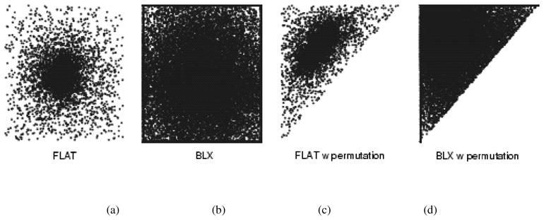
Scatter plot of evaluated parameter vectors in artificial 2 variate case when no selection pressure is present. (a), (b) Situation without constraints and (c), (d) when variate in x axis is constrained to be smaller than variate in y axis.
B. Permutation Operator
We ensure that
| (14) |
after recombination (for multivariate FMMs the ordering is to be understood with respect to some prespecified component of the mean vector). This is done by permuting the variables according to the following permutation operator.
For all index pairs u, v where u < v ≤ K do the following. If μu > μv, then swap μu and μv, Σu and Σv, pu and pv.
This operator implements the constraint (14) in an effective manner as compared to penalty methods typically used for the constrained optimization with real coded GAs [43]. The reason for the constraint is that after a permutation of the classes the likelihood of the data remains the same whereas the interpretation of the FMM changes as can be seen from (2) and (7). This kind of identifiability problem, referred to as label switching in [38], is encountered because the intensities of the pure voxel classes are all modeled with the same parametric distribution. Therefore, without extra information, the FMM does not include a possibility to interpret the classes correctly. For example in T1-weighted MR data, white matter (WM) intensities are greater than gray matter (GM) intensities on average. This kind of information can be used to interpret the classes in an FMM as actual tissue classes instead of just as classes numbered from 1 to K. This again is necessary if we would like to embed specific constraints to the FMM parameters based on neuroanatomical prior knowledge. As an example, we could constrain that there must be at least 50% of GM in the brain. Then, it is simple to constrain the relevant mixing parameter to be greater than 0.5. However, to decide which is the mixing parameter of the GM class, it is necessary to enforce the constraint (14) or, equivalently, to apply the permutation operator.
Additionally, the permutation operator reduces the size of the search space, thus decreasing the computational cost of the FMM parameter estimation. This is because there are K! possible orderings of the means of tissue classes and, with the permutation operator, we allow only one of them. The search space for the GA with a two-variable artificial optimization problem is visualized in Fig. 2.
For real coded GAs, the permutation operator forbids the recombination with two similar parents which only have their classes switched. This would result in an offspring completely different from the parents although the parents themselves were essentially equal, which is not desirable. In our experiments, we have not found that extending the permutation operator to PV classes would be beneficial although pure tissue classes are permuted.
C. Fast Implementation
The likelihood function in (3) needs to be evaluated numerous times during our GA. Hence, a notable speed up can be achieved by using a well-known connection between maximum-likelihood and the Kullback–Leibler divergence [44], [45]. This acceleration technique is only applicable for 1-D FMMs and hence we restrict our attention to them in this subsection.
The Kullback–Leibler divergence between the true pdf g(·) and the parametric density f(·|θ)is
| (15) |
Minimizing this divergence with respect to θ is equivalent to maximizing the likelihood (3) when the number of data points N tends to infinity [44]. By replacing the integral in (15) by its trapezoidal approximation and g(·) by its Parzen estimate ĝ(·) [31], we get a faster way to obtain the ML estimate
| (16) |
| (17) |
In this paper, we select M = 100 and zj = mini xi + (j − 0.5)/(M)(maxi xi − mini xi). The Parzen estimates ĝ(zj) are computed using Gaussian window functions with the standard deviation of (maxi.xi − mini xj)/M. This results in a speed increase by the factor N/M. For a typical MR image of human brain, this factor can be 10 000. Obviously, the EM algorithm can be sped up with the same technique and this kind of speed up strategy has been previously proposed in [46]. However, in [46] histograms were considered instead of the Parzen density estimates. Therefore, our approach is more general and better suited for real valued data. We use this approach to accelerate also the EM algorithm in this paper.
D. Covariance Matrices
In this subsection, we briefly discuss our coding scheme for covariance matrices in d-dimensional case and describe how to ensure that they are positive-definite as required. Each covariance matrix Σk is coded by d2 + d real scalars using concepts from the generation of random correlation matrices [47]. Let the diagonal matrix D = diag[σ11, …, σdd], where σuu is the standard deviation of the uth dimension of the class k. We can write
| (18) |
where R is a correlation matrix and the rows Q of have unit length. (R = QQT is a valid correlation matrix if and only if the rows of Q have unit length [47].) The covariance matrices are coded using variables , u = 1, …, d; quv, u, v = 1, …,d, which are subject to constraints
| (19) |
| (20) |
To ensure that constraints (20) are satisfied under the blended crossover, we apply a normalization scheme similar to that used for mixing parameters.
E. Hybrid Algorithm for Multidimensional FMMs
A drawback of the GA for the d-dimensional FMMs is that the acceleration technique described in Section III.C is not applicable and the speed of the algorithm can be too slow. Therefore, we introduce a faster alternative (called hybrid-GA) which benefits both the robustness of the GA in the 1-D case and the self-annealing behavior of the EM algorithm. Note that this algorithm is different from the GA + EM algorithms [18], [19], as it was explained in Section I.
The hybrid-GA consists of d runs of the GA for the 1-D FMMs (step 1) followed by the d runs of the EM starting from the results from Step 1 (Step 2).
-
Step 1
Denote xi = [xi1, …, xid]T. Given the data {x1, …, xN: xi ∈ ℝd}run d GAs. jth GA is run with the input {x1j, …, xNj} for j = 1, …, d and the resulting parameter vector is denoted by θ̂j. From these, we compute the probabilities P(k|xij, θ̂j) that xij belongs to the class k.
-
Step 2
For each j = 1, …, d, we start an EM algorithm from the initialization provided by πik(0) = P(k|xij, θ̂j) (see Section II-C). All the runs use the d-dimensional input data {x1, …, xN: xi ∈ ℝd}. The result of the EM algorithm with the highest log-likelihood is selected as the result of our hybrid-GA.
This algorithm is rooted in the fact that the components of a multidimensional Gaussian random vector are normally distributed. Furthermore, the variances and the means of the components of a random vector are given by the corresponding components of the mean vector and the covariance matrix of the random vector. Similar reasoning obviously holds for densities of the PV classes which, according to the mixel model, are constructed as weighted sums of independent Gaussian random variables.
We claimed that the algorithm benefits from the self-annealing behavior of EM. Indeed, if in the first step any two or more tissue classes are not well separated based on, say, the jth components of the input data, then the probabilities for these tissue classes are approximately equal provided that the parameters for the 1-D mixture have been correctly estimated. This leads to the EM algorithm which is partially based on the high entropy initialization. However, those tissue classes which are well separated by the jth variable should be well initialized and the optimization problem should be easier than when starting from the “pure” high entropy initialization described in Section II-C.
Obviously, there are FMMs whose parameters cannot be well estimated by the hybrid-GA algorithm. For example, if tissue classes would have the same mean vectors and they would be separable only based on different covariance matrices, then the hybrid-GA algorithm would be unlikely to estimate the parameters accurately. However, in voxel classification within neuroimaging, it is reasonable to assume that the means of different tissue classes are not equal.
IV. Experiments and Results
A. Experiment Settings
1) Algorithms to be Compared
We tested the algorithms with five sets of synthetic and real brain imaging data. The algorithms to be compared with 1-D data were: 1) our algorithm (BLX-GA) with BLX-0.5 operator and the permutation operator; 2) a GA similar to [14] with the flat crossover and without the permutation operator (FLAT-GA); 3) the EM-HE algorithm, either standard or the PVE modification, where the HE suffix refers to the high entropy initialization described in Section II-C. The FLAT-GA algorithm was otherwise exactly the same as our BLX-GA algorithm except that it used the flat crossover and it did not contain the permutation operator. This algorithm was studied to make our novel contributions clearer. With synthetic data, we additionally considered a GA + EM algorithm [18], [19].2 The population size for the algorithm was selected so that computational demands during one generation of it (both GA and EM steps) corresponded to computational demands during one generation of other GAs. For this, we have assumed that one iteration of EM corresponds to one evaluation of the likelihood function. This is a lower bound for the complexity of EM.
With multidimensional data, we compared the BLX-GA, the hybrid of BLX-GA, and the EM algorithm, the EM-HE algorithm with the high entropy initialization and GA + EM. The classes were ordered in the same way as described in Section III-B after the initialization and after the parameter estimation with FLAT-GA, EM-HE, and GA + EM. Hence, the improvements by BLX-GA were not due to the label switching problem.
All the tested algorithms are stochastic, that is, they contain a nondeterministic component and may lead to different results in different runs. Hence, one run of a particular algorithm may well give an erroneous picture of the performance of that algorithm, and the experiments concerning stochastic (optimization) algorithms require multiple runs of a single algorithm. Here, we repeated each experiment with each dataset 50 times.
2) Material and Error Criteria
The first dataset consisted of simulated 1-D and 3-D Gaussian mixtures that contained no PV classes. These data were studied because we wanted to compare our algorithm and others when PVE does not complicate the FMM.
Second, we tested the algorithms using image data from the BrainWeb database of the Montreal Neurological Institute [48], [49]. The quality of the results of different algorithms with these synthetic data were measured using the misclassification rate between the true classification and the classification by the estimated parameters. The misclassification rate is defined as the ratio of the number of misclassified voxels to the total number of voxels. (With the BrainWeb data, only the voxels within the brain were considered.) This measure was selected because it gives a rather complete and easily interpretable picture of the quality of results. The misclassification rate depicts the quality of the whole classification with a single value unlike the Dice or Jaccard coefficient (see [27]) which encodes only the quality of the classification with respect to a single tissue class.
The algorithms were tested with real image data from T1-weighted MRI of human brain, T2-weighted MRI of mouse brain, and parametric FDG ([18F] fluorodeoxyglucose) PET. With these data, we tested the reproducibility of the results between different runs of the algorithms. This is important because the algorithms involve random components. We estimated the FMM parameters of the image data starting from a random initialization and tissue classified the image. This was repeated 50 times as with the synthetic data. Based on the 50 tissue classified images, the average classification was constructed by deciding the label of each voxel by a majority vote. Then, the reproducibility was measured by computing the fraction of voxels (in 50 classifications) classified differently than in the average (majority vote) classification. Note that averaging the classification results was done purely for the display of the average classification results by stochastic algorithms and the study of the reproducibility of classification results. We do not suggest using such a scheme in practice. In addition to the reproducibility study, we computed the Kullback–Leibler divergences (17) between the estimated parametric mixture densities and true densities of the whole data. Since we aim to minimize the Kullback–Leibler divergence (17), the divergence is an indicator of the success of an algorithm in the optimization problem. There is no bijective correspondence between the Kullback–Leibler divergence and the quality of classification. However, since the ground truth is not available, we have few other choices in quantifying the results of the algorithms with these data.
B. Experiments With Synthetic Data Without PVE
In the first experiment, the properties of our GA are demonstrated by considering a three-class 1-D FMM parameter estimation problem and a six-class 3-D problem. There were no partial volume classes (i.e., K′ = 0).
The 1-D FMM whose parameters were to be estimated is shown in Fig. 3. This FMM constitutes a difficult parameter estimation problem although the optimal decision boundaries for the task are linear. The Bayes error for this classification task is 11.8%. We drew randomly 10 000 data points according to this FMM, estimated the parameters of the FMM by different algorithms, and then classified the points according to the Bayes classifier.
Fig. 3.

(a) Plot of mixture density for parameter estimation experiment, (b) box-plot of resulting misclassification rates, and (c) statistics of misclassification rates with different algorithms and 50 initializations). Column “min” (respectively “mean,” “median,” and “max”) gives minimum (mean, median, maximum) misclassification rate resulting from 50 random initializations. Algorithms are: GA with BLX-0.5 and permutation operators (BLX-GA); GA with BLX-0.5 but without permutation operator (GA-NPO); GA with BLX-0.0 and without permutation operator (FLAT-GA); GA with BLX-0.0 and with permutation operator (FPO-GA); EM with a random initialization (EM); EM with high entropy initialization (EM-HE); GA + EM hybrid [19], [18] (GA + EM).
With this problem, we demonstrate the behavior of the standard EM algorithm with randomly initialized parameter vectors, BLX-GA without permutation operator, and FLAT-GA with permutation operator in addition to BLX-GA, FLAT-GA, GA + EM, and EM-HE. Our purpose is to show that: 1) the high entropy initialization of the EM algorithm has significant advantages over the random initialization; 2) the permutation operator is an important component of our GA and it works better when combined with the BLX-0.5 crossover operator than with the flat crossover.
The statistics and the box-plot of misclassification rates using different parameter estimation algorithms are shown in Fig. 3. BLX-GA and GA + EM achieved best results on average as can be seen by inspecting median and mean misclassification rates in Fig. 3. These are close to the Bayes error, which defines the best possible performance. The misclassification rates for FLAT-GA and BLX-GA without permutation operator (NPO-GA) were worse than misclassification rates for BLX-GA. In particular, the improvement by the permutation operator was notable. Note that combined with the flat crossover, the improvements by the permutation operator were modest. The EM-algorithm worked well for some initializations. However, a completely random initialization rarely yielded a successful result. Instead, the high entropy initialization described in Section II-C yielded successful results on most runs but not as often as BLX-GA and GA + EM. This can be seen from the box-plot or from mean misclassification rates in Fig. 3.
With EM-HE, BLX-GA, and GA + EM good optimization results (i.e., high likelihood values) implied low misclassification rates as was expected. This was not the case with FLAT-GA which yielded lower likelihood scores than EM-HE, GA + EM, and BLX-GA. With FLAT-GA, a higher likelihood score did not necessarily imply a better classification result and classification results with a low misclassification rate did not imply good parameter estimates. For example, the average absolute error in mixing parameters estimated by the run with the lowest misclassification rate was 0.0572 for FLAT-GA while it was only 0.0171 for BLX-GA. The misclassification rates for these runs were equal (11.8%). Similarly, other parameters were poorly estimated by FLAT-GA. Because one cannot deduct the quality of the classification based on the likelihood score, this renders FLAT-GA as a poor candidate for multistart optimization algorithms, where the same algorithm is run multiple times and the result of the run with the highest log-likelihood is selected as the final result [50].
Second, we tested multidimensional BLX-GA and hybrid- GA introduced in Section III-E against the EM-HE algorithm and GA + EM. The test-data contained 20 000 samples from 3-D FMM with six normally distributed components, see Fig. 4. The component densities featured strong correlations among the three variates. That is, the covariance matrices had significant off-diagonal components. The Bayes error of this clustering problem was 12.8%. The population size of GA + EM was tuned corresponding to BLX-GA, which is the slowest algorithm of those studied.
Fig. 4.

Densities of simulated test data marginalized with respect to (a) third variate and (b) first variate. Density marginalized with respect to second variate is as density in (a).
The results of this experiment are listed in Table I. The hybrid- GA performed very well. All the runs of it were successful in that they resulted in an error close to the Bayes error. The direct generalization of the BLX-GA algorithm was not as successful as can be seen from Table I. Its median misclassification rate was roughly 2.5 times the Bayes error. With the direct generalization, the population size of 330 was applied. This population size was derived from the population size of the 1-D experiments based on the number of additional variates in the optimization problem. It is largely a compromise between the quality of results and feasible computation time. A larger population size would be likely to improve results. The EM-HE algorithm performed worst here, resulting in only one successful run out of 50. The GA + EM was more successful on average than EM-HE and BLX-GA. However, it was still clearly less successful than our hybrid-GA: the worst run of hybrid-GA resulted in the misclassification rate (14.1%) that EM+GA rarely achieved.
TABLE I.
Misclassification Rates in Percents With Different Algorithms and 50 Random Initializations for Multidimensional FMM Experiment. Hybrid-GA Is Hybrid of GA and EM-Algorithm Described in Section III-E. Other Notation Is as in Fig. 3
| min | mean | median | max | |
|---|---|---|---|---|
| BLX-GA | 18.7 | 32.8 | 31.8 | 59.3 |
| hybrid-GA | 13.9 | 13.9 | 13.9 | 14.1 |
| EM-HE | 14.2 | 59.2 | 59.1 | 82.5 |
| EM+GA | 13.9 | 25.2 | 21.0 | 83.9 |
C. Experiments With BrainWeb Images
In this experiment, the algorithms were compared using the simulated brain MRI images from the BrainWeb database by the Montreal Neurological Institute http://www.bic.mni.mcgill.ca/brainweb [48], [49]. We applied the images with no intensity nonuniformity, with the resolution of 1 × 1 × 1 mm, and with the image size of 181 × 217 × 181. The images were simulated with T1 and T2 weighted as well as proton density (PD) pulse sequences. See Fig. 5 for intensity distributions and examples of image cross sections. The brain volume was extracted based on the ground-truth. The pure voxel classes were WM, GM, and cerebro spinal fluid (CSF). The PV classes were CSF/GM and WM/GM. The class background/CSF was not included due to its negligible effect to the FMM.
Fig. 5.

Examples of BrainWeb images and their intensity distributions. Noise level is 5 %.
The results are presented in Table II. As can be seen, both GAs were more reliable than the EM-algorithm with the high entropy initialization. Especially, this tendency was clear with T2 and PD images where the overlaps between the component densities were greater than with T1 images and where the intensity densities had no clearly identifiable peaks corresponding to the pure tissue classes. With T2 and PD images, the best misclassification rate with EM-HE was typically higher than the average misclassification rate by BLX-GA. With T1-weighted data, EM-HE featured slightly worse average behavior than genetic algorithms because of some runs of it failed completely. However, the lower computational complexity of EM-HE as compared to GAs equalized this slightly worse average performance.
TABLE II.
Misclassification Rates From 50 Runs With BrainWeb Data. For Each Algorithm Minimum Misclassification Rate and Average Misclassification Rate is Listed. Values Are in Percents
| pulse seq. noise % | T1 | T2 | PD | ||||||
|---|---|---|---|---|---|---|---|---|---|
| 3 | 5 | 7 | 3 | 5 | 7 | 3 | 5 | 7 | |
| BLX-GA mean | 4.1 | 6.2 | 9.6 | 8.8 | 15.2 | 20.8 | 16.1 | 28.3 | 36.1 |
| BLX-GA min | 4.1 | 6.1 | 9.5 | 8.2 | 14.4 | 19.8 | 13.6 | 23.8 | 31.2 |
| FLAT-GA mean | 4.2 | 6.4 | 9.8 | 12.5 | 16.2 | 20.4 | 19.0 | 29.8 | 37.2 |
| FLAT-GA min | 3.6 | 6.0 | 9.5 | 7.9 | 14.3 | 19.7 | 13.7 | 25.1 | 33.0 |
| EM-HE mean | 8.2 | 7.1 | 11.3 | 35.0 | 44.2 | 37.8 | 44.4 | 47.1 | 50.2 |
| EM-HE min | 4.1 | 6.1 | 9.6 | 9.9 | 20.1 | 19.8 | 22.2 | 30.3 | 36.8 |
The mean performance of BLX-GA was consistently better than that of FLAT-GA, see Table II. This difference was especially clear with the T2-weighted and PD images with the lowest noise level. Sometimes, the best misclassification rates by FLAT-GA were remarkably low. However, as in the previous experiment, the best performance in terms of the misclassification rate was never achieved with the best optimization results, and hence choosing the best run among several ones would be difficult. However, in this instance BLX-GA also suffered from the same difficulty. With EM-HE and T1 weighted data, a high likelihood value typically resulted in a low misclassification rate. However, with T2 and PD images, this was not the case. These observations suggest that PVE brings forward an additional source of difficulty in voxel classification. We note that all our assumptions are in line with the simulations except that we used the Gaussian model for the pure tissue types instead of the Rician model.
D. Experiments With Pathologic Brain MRI
In this experiment, the algorithms were studied using 3-D T1-weighted MR brain scans of healthy and diseased (Alzheimer’s disease (AD), schizophrenia, and childhood schizophrenia) subjects (Fig. 6). (Imaging devices, and image and voxel dimensions varied.) The images were corrected for the intensity nonuniformity using the N3 method [12]. The brain was extracted using the Brain Surface Extractor [27] (healthy, schizophrenia) using the Brain Extraction Tool (childhood schizophrenia) [51] or manually (AD).
Fig. 6.

Top row: Axial cross sections of images applied in reproducibility test. Middle row: Axial cross sections of average voxel classifications that were decided by majority vote from 50 random initializations for BLX-GA parameter estimation. The “normal” image is the same as in our example in Fig. 1. Images are in native space. In bottom row intensity distributions of images are shown.
As can be seen from Table III, the percentages of brain voxels classified differently compared to the average (majority vote) classification were typically lowest with the EM-HE algorithm. This could be partly because its stochastic nature stems only from a random initialization while other algorithms have more random components. The reproducibility of BLX-GA was better than FLAT-GA on average. With the image of the AD subject, however, the ranks of the algorithms were opposite, with the EM-HE algorithm achieving reproducibility of only 16.5%. The EM-HE algorithm appeared to be the best one when looking at the Kullback–Leibler divergences in Table III. However, the resulting Kullback–Leibler divergences by BLX-GA were similar to those with EM-HE. The Kullback–Leibler divergences produced by FLAT-GA were usually at least ten times larger than with BLX-GA or EM-HE. Note that with all images, there was a noticeable peak in the intensity distribution for the GM and WM classes (see Fig. 6).
TABLE III.
Average Kullback–Leibler Divergences and Reproducibility of Classification Results in Percents From 50 Runs of Each Algorithm With Real Image Data. Lower Values Mean Better Results. Abbreviation “SZ” Stands for Schizophrenia. Cf. Section IV-A for Experiment Settings. With Mouse MRI, Kullback–Leibler Divergences by BLX-GA Are Not Fully Comparable to Others Because of Imposed Constraints (cf. Section IV-E)
| Reproducibility % | ||||||||||||
|---|---|---|---|---|---|---|---|---|---|---|---|---|
| Human MRI | Mouse MRI | FDG-PET | ||||||||||
| image | Normal | AD | SZ | Child SZ | 1 | 2 | 3 | 4 | 1 | 2 | 3 | 4 |
| BLX-GA | 2.8 | 5.3 | 1.2 | 2.9 | 5.1 | 0.2 | 0.3 | 0.2 | 5.7 | 3.7 | 5.7 | 11.8 |
| FLAT-GA | 6.0 | 3.4 | 3.4 | 3.8 | 10.3 | 5.2 | 5.3 | 7.7 | 4.9 | 4.1 | 4.5 | 4.1 |
| EM-HE | 2.4 | 16.5 | 0.6 | 0.4 | 3.1 | 10.9 | 4.9 | 17.5 | 26.6 | 24.1 | 0.7 | 25.0 |
| Kullback-Leibler | ||||||||||||
| BLX-GA | 0.0057 | 0.0077 | 0.0015 | 0.0063 | 0.0132 | 0.0173 | 0.0130 | 0.0204 | 0.0030 | 0.0022 | 0.0039 | 0.0030 |
| FLAT-GA | 0.0879 | 0.0252 | 0.0512 | 0.0774 | 0.2417 | 0.0519 | 0.2578 | 0.2970 | 0.0066 | 0.0100 | 0.0093 | 0.0101 |
| EM-HE | 0.0041 | 0.0072 | 0.0014 | 0.0005 | 0.0003 | 0.0003 | 0.0007 | 0.0004 | 0.0156 | 0.0129 | 0.0020 | 0.0289 |
The average tissue classifications, decided by the majority vote, of BLX-GA are shown in Fig. 6. In visual inspection, these appear to be of good quality.
E. Experiments With Mouse Brain MRI
In addition to tissue classification in human brain MRI, which is a relatively well-studied problem, we studied the applicability of the BLX-GA for tissue classification of mouse brain MRI. The material consisted of four T2-weighted brain MR images of mouse brain which were acquired using an 89-mm vertical bore 11.7T Bruker Avance imaging spectrometer. The image dimensions were 256 × 256 × 512 and the voxel size was 0.05 × 0.0375 × 0.05 mm.
Multiple sclerosis (MS) studies in humans rely heavily on MRI as a measure of disease progression, quantifying the progress of disease by calculating gray- and white-matter loss [52], [53] and changes in the brain parenchymal fraction. These studies have been greatly facilitated by automated tissue classification algorithms [52]. Analysis of gray and white matter structure in the most commonly used mouse model of MS, experimental autoimmune encephalomyelitis (EAE), has lagged behind due to a lack of automated tools. Image segmentation, namely tissue classification, on mouse MRI has relied on highly labor intensive manual delineation. An automated image segmentation tool that will work on mouse MRI data would greatly accelerate the pace of analysis and discovery.
With these experiments, our purpose is to demonstrate the added flexibility of BLX-GA by the permutation operator. The permutation operator allows imposing constraints to the specific components of FMM such as there must be at least 60% of the gray matter in a brain. Imposing such constraints is not possible in FLAT-GA without permutation operator. However, with EM-HE, such constraints could in principle be imposed using the maximum a posteriori (MAP) framework (see [39]), but it could be hard to target component densities or mixing parameters with the specific biological interpretation within the MAP framework.
We applied an FMM consisting of four pure tissue classes and three PVE classes. (See Fig. 7 for examples of intensity distributions.) The FMM for this problem is still preliminary and further study is needed to decide upon the best model; however, this model produced good experimental results with our GA. Two of the component densities modeled gray matter voxels, whose intensities appears to be different in cerebellum and in the gray matter structures within cerebrum. However, parts of the cortex fall also to the cerebellum class. As these intensities overlap heavily, the segmentation between these gray matter structures does not appear possible without applying spatial information and therefore we consider gray matter to be modeled with a FMM with two pure components and one PV class. The other two classes were for white matter and CSF. PV classes were WM/cerebral GM, cerebral GM/cerebellar GM, and CSF/cerebellar GM. The classes WM/cerebellar GM and CSF/cerebral GM were not included to avoid identifiability issues. The cerebral GM was required to contain 50% of voxels with BLX-GA and the cerebellar GM (also containing parts of the cortex) was required to contain 10% of them. With other algorithms no constraints were imposed.
Fig. 7.
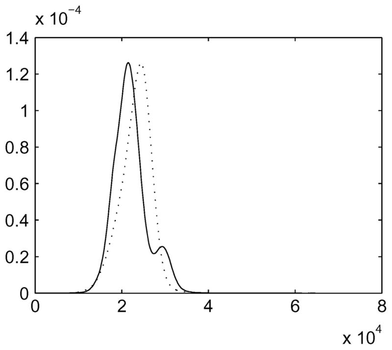
Examples of intensity distributions of T2-weighted mouse brain MRI; solid line: image 1 and dotted line: image 4.
Table III lists the reproducibility percentages along with the resulting Kullback–Leibler divergences for different methods averaged over 50 runs. From Table III, it can be seen that the Kullback–Leibler divergences of the EM-HE were the lowest and those of the FLAT-GA were the highest. However, note that Kullback–Leibler divergences by BLX-GA are not fully comparable to others because of the imposed constraints. The lowest achievable Kullback–Leibler divergence is lower in the unconstrained case than in the constrained case. Indeed, while EM-HE was successful in the minimization task, the classification results by it were not biologically meaningful. This is demonstrated in Fig. 8, where the majority vote averages of voxel classifications of the image 4 are shown. The component density with the lowest mean included typically both white matter and gray matter, and the component density with the highest mean included typically both CSF and gray matter; this rendered the classification results useless. On the other hand, BLX-GA gave very accurate results with three of the four images in the sense that little could be improved if the voxels labels are assumed to be independent, see Fig. 8 for an example. Also, the results by BLX-GA were highly reproducible in three cases out of four suggesting that our FMM for this problem is stable (i.e., there are no serious identifiability problems) when the fraction of gray matter in brain has been constrained. We conclude that our GA could be applied for tissue classification in mouse brain imaging, at least when combined with a spatial modeling technique such as an MRF.
Fig. 8.

Examples of average voxel classification results with mouse MRI. From left, voxel classification by BLX-GA and average voxel classification by EM-HE of same image. White color denotes CSF, light gray the gray matter, and dark gray the white matter. From top, coronal, horizontal, and sagittal cross-section views. Sagittal cross section is scaled differently from other cross sections for better fit into figure.
The poor Kullback–Leibler divergences by FLAT-GA were probably due to tendency of FLAT-GA to produce FMMs with equal mixing proportions. This is due to the crossover operator which overemphasizes exploitation over exploration and concentrates the search in the “center” of the space of admissible solutions as explained in Section III-A.
F. Experiments With Parametric FDG-PET
We applied the algorithms to the parametric FDG-PET images where partial volume effect is even a greater problem than within MRI. These images here present an extreme situation where high noise levels and partial volume effects possibly create more severe identifiability problems than label-switching (See Section III-B).
All four PET acquisitions were made with the GE Advance scanner (GE, Milwaukee, USA). The pixel by pixel Patlak model [37] was applied to the FDG sinograms to produce parametric images. The parametric sinograms were reconstructed with the iterative MRP method to the cross section image size of 128 × 128 [54]. The voxel size was 1.72 × 1.72 × 4.25 mm. An example of an FDG-PET image and its intensity distribution is shown in Fig. 9. The brain was extracted automatically by the DM-DSM method [55], [56].
Fig. 9.

Examples of FDG-PET classification results: (a) intensity distribution, (b) transaxial image plane, (c) classification results using BLX-GA, (d) FLAT-GA, and (e) EM-HE.
The FMM consisted of two pure tissue classes (GM and WM) and two PV classes (GM/WM and GM/background). The class background required for one of the PV classes was normally distributed with mean 0 and the same variance as the GM class. In the classification stage (4), the class background/GM was ignored because the differentiation between it and the WM class requires information about the location of the voxel in the image.
The quantitative results with different algorithms are listed in Table III. Here, BLX-GA produced the best Kullback–Leibler divergences with images 1, 2, and 4. With the image 3, the Kullback–Leibler divergence of the EM-HE was the lowest. The results were surprisingly reproducible with both GAs given the difficulty of the classification task. On the other hand, the EM-HE algorithm produced very different results depending on initialization resulting typically in only half of the reproducibility of completely random classification. The Kullback–Leibler divergences, listed in Table III, were typically the lowest with BLX-GA and the highest with EM-HE.
Examples of the average classification results using different algorithms are shown in Fig. 9. These voxel classifications appear to be of high quality in visual inspection. Note that with PET the applied image reconstruction method affects considerably the visual appearance and the quality of images. Therefore, it is likely that the visual appearance of the voxel classifications would differ if the images were reconstructed with, e.g., the filtered back projection method.
G. Computational Complexity and Summary of Results
In this section, we summarize the results of the previous subsections and discuss the merits of the different algorithms in relation to their computational efficiency. The algorithms in this paper were not optimized in their parameters for the computational efficiency and that is why giving the number of function evaluations required for the optimization of the parameters of a particular FMM might be misleading. However, the EM-HE algorithm is clearly faster than BLX-GA and therefore it is important to identify the circumstances where multistart EM-HE (i.e., running EM-HE multiple times and selecting the run with the highest likelihood score as the final result) is a better option than BLX-GA. As indicated earlier in this section, FLAT-GA is a poor candidate for the basis of a multistart algorithm and therefore we restrict our attention to the comparison of BLX-GA and EM-HE. Our C-implementation of BLX-GA, the slowest of the algorithms, runs in approximately 1 min even for a high-resolution MR image when accelerated as described in Section III-C and hence a single run of any algorithm in the 1-D case is computationally feasible.
For simple tissue classification problems, where each pure tissue class is characterized by a clear peak in the image histogram such as with T1 weighted MR images, running EM-HE multiple times would be advisable according to our experiments. For more complicated tissue classification problems arising e.g., with T2 and PD MR-images and with FDG-PET, BLX-GA is the preferable option. This because of two reasons. Referring to the BrainWeb experiments with T2 and PD images, BLX-GA yielded better classification results on average than the best classification by EM-HE. Also, multistart strategies were not a reasonable option with any of the algorithms with T2 and PD BrainWeb images because the ranks of runs based on the likelihood scores and the misclassification rates of the runs did not correlate enough. We still demonstrate the relative speed of EM-HE and BLX-GA with an example from experiments with BrainWeb data and the 5% noise level. Here, BLX-GA required on average 60, 669, and 254 generations until convergence for T1, T2 and PD images, respectively. In the same experiments, EM-HE required on average 896, 4536, and 640 iterations. Thus, if one accepts the approximation that one iteration of EM corresponds to one function evaluation, EM-HE was (on average) 6.7 (T1), 14.7 (T2), and 38.0 (PD) times faster than BLX-GA. Note that the acceleration technique of Section III-C is necessary with EM to obtain results faster than with GAs.
In a multidimensional case, the main source of time consumption of the hybrid-GA algorithm, if there is a large number of data points, is running the EM algorithm d times. The time consumption of the GA part is negligible because of the acceleration procedure of Section III-C, provided that the number of data points is large. Hence, the time consumption of the hybrid is about d times of that of EM-HE. The pure BLX-GA in the multidimensional case was much slower. The GA+EM took typically a fewer number of generations (on average 36.14 generations, each consisting of 66 times five EM iterations) to converge than BLX-GA to which the complexity of GA + EM was tuned to. However, our hybrid-GA (on average 9453 EM-iterations) was still faster than GA + EM. Hence, in the multidimensional case, hybrid-GA is preferable also when computation time is taken into account.
V. DISCUSSION
We have presented a global real coded GA for the FMM parameter estimation to be used in neuroimaging applications. The motivation for this algorithm stems from the requirement to solve divergent voxel classification problems in brain research. Our GA contained two novel features compared to the previous GA-based approaches for FMM optimization: 1) we applied the blended crossover which reduces the problem of the premature convergence to its minimum; 2) a completely new permutation operator was introduced. In addition, we introduced two algorithms for optimization of multidimensional FMMs out of which the hybrid of the GA and EM algorithm was found to be superior both in terms of the performance and computation speed.
Although the global convergence of our algorithm cannot be proven, the algorithm is not sensitive to its initialization which makes it particularly useful in cases where a well-principled initialization for a local algorithm, such as the EM algorithm, is not available. (See [50] for general account of the complexity of global optimization problems.) Moreover, the parameters for arbitrary FMMs can be estimated, since the algorithm does not require any assumptions about the parametric models for the component densities. This is important in many brain imaging applications where, e.g., the influence of the partial volume effect is large. In addition, our algorithm allows constraining of values of the specific parameters to lie within a certain range. This was shown to be useful with a tissue classification task of MR images of mouse brain, where we constrained the amount of gray matter in the brain. Constraining the ranges of the specific parameter values is likely to be useful in applications where the parametric FMM does not precisely coincide with the biological interpretation of the data.
We compared our GA with a GA similar to the one proposed in [14] (FLAT-GA) and with the self-annealing EM-algorithm (EM-HE). We tested the algorithms for the voxel classification problems with a variety of synthetic and real 3-D image data from MRI and PET. The main conclusions were as follows. 1) Our GA outperformed FLAT-GA in every experiment. 2) GAs outperformed the EM algorithm where the FMM to be optimized featured heavily overlapping component densities in the 1-D case; otherwise, the EM with the high entropy initialization appeared to be a reasonable choice. 3) The hybrid-GA algorithm for multidimensional FMMs was superior compared to the pure GA, GA + EM, and EM-HE algorithms.
The tissue classification in human MRI is a well-studied problem. The automated algorithms for this problem are vital for many large scale studies of the human anatomy in health and disease. The global FMM optimization approach for tissue classification has the advantage of not requiring restricting assumptions about the underlying anatomy. This can be important when analyzing images of the pathological brain, and we have demonstrated the viability of the approach in some important disorders.
There are few tools available for the automated tissue classification of mouse MRI data. As indicated in Section IV-E, an automated image segmentation tool that will work on mouse MRI data would greatly accelerate the pace of analysis and discovery in the study of EAE, the mouse model of MS. Though many tools have been developed for use in human MRI analysis, they often make assumptions about the underlying data, such as the requirement of a fixed range of intensity values for each tissue type (e.g., [57]), parameter estimation techniques that rely on human MRI specific features (e.g., [27]), or the requirement of the images to lie in a stereotactic space (e.g., [7]). These assumptions rely in many cases on having T1-weighted or human brain MRI. Although completely reasonable for a particular application, they might not be easily adapted for the tissue classification of different types of brain images. In this paper, we demonstrated that with the addition of a single constraint on gray matter content in the brain, our FMM optimization approach is appropriate for mouse tissue classification.
The voxel classification of brain PET images is a problem of increasing importance. As the resolution of PET scanners and the number of voxels in images increase, automatic approaches for region of interest (ROI) delineation will become necessary as the manual delineation of ROIs will become too burdensome and ineffective. In this paper, we have studied the voxel classification of the parametric FDG-PET images. Our FMM optimization algorithm yielded successful results for this application highlighting the generality of the proposed method for the FMM optimization.
In pattern recognition literature, there exist methods for avoiding the local maxima problem with the FMM optimization task. These methods are typically extensions of the EM algorithm or hybrid algorithms combining EM with some hill-climbing methods. The deterministic annealing-based EM, which shares a similarity with the self-annealing EM studied in this paper, was studied in [41]. In [58], the authors presented a split and merge EM algorithm which avoids local likelihood maxima by splitting component densities into two or merging two component densities into one. The algorithm can be roughly described as a multistart EM algorithm, where the result of the conventional EM algorithm is improved by reinitializing the algorithm by a sophisticated reinitialization process. A drawback of the algorithm was detected and corrected in [59]. In [11], the authors suggested integrating the model selection (the selection of the number of the mixture components) and parameter estimation. At the same time, a considerable reduction in the initialization sensitivity was achieved by starting with a high number of components and merging components as the algorithm proceeded.
In [18] and [19], the authors combined a GA based on the simple crossover and the EM algorithm. These algorithms are rather different in spirit compared to our GA. They apply a simple crossover operator to perform the exploration in the parameter space in order to avoid the tendency of the EM to find only the local likelihood minimum instead of the global one. The simple crossover cannot exploit the continuity in the parameter space (see [21]), and the algorithms compensate for this by using EM for the local improvement of the parameter values. In contrast, we apply the BLX-0.5 operator simultaneously for the exploration and exploitation (improving parameter values locally). We compared our BLX-GA to these GA + EM algorithms in Section IV. The algorithms performed equally well with the 1-D problem. However, in the multidimensional case, our hybrid-GA featured a superior performance to GA + EM.
All of the mentioned algorithms can be considered as extensions of the EM algorithm and therefore they do not directly offer the same flexibility as our method when constraining the mixing parameters. Moreover, a major aim in many of these algorithms is the estimation of the correct number of component densities in the FMM which is not, in itself, vital in unsupervised voxel classification within medical imaging. That is, the algorithms for unsupervised voxel classification with a variable number of component densities would have to include an automatic mechanism for correctly matching the component densities with the tissue types. Selecting the correct number of tissue types a priori is usually possible when considering brain imaging for the neuroscientific research where the effects of subject pathology to the brain anatomy are known, at least on the gross level.
VI. CONCLUSION
We have introduced a real coded genetic algorithm for solving challenging FMM optimization problems arising in neuroimaging. The challenge of these problems is due to several local optima yielding local optimization algorithms sensitive to their initializations. Our algorithm has been demonstrated to be capable of solving accurately different kinds of FMM optimization problems for the voxel classification purposes. We have compared experimentally our algorithm to other FMM optimization algorithms capable of avoiding the initialization sensitivity problem and identified the situations where the use of our algorithm is recommendable. In general, our algorithm was the most consistent and accurate of the algorithms compared, although in few applications the usage of a different method was found recommendable for computational reasons. The initialization sensitivity is a serious problem hampering automated image analysis procedures based on a cost function optimization in general and it restricts the applicability of these procedures to large datasets required in modern neuroscientific studies. In particular, many FMM optimization problems are characterized by the several local optima. Consequently, our algorithm can be used to fully automate many FMM optimization tasks which will help to develop automatic image analysis procedures for brain imaging.
Acknowledgments
The PET images for this study were provided by the Turku PET Centre, Turku, Finland. The GA-FMM software tool can be found at http://www.loni.ucla.edu/CCB/Software and http://www.cs.tut.fi/~jupeto/gamixture.html. Information on the National Centers for Biomedical Computing can be obtained from http://nihroadmap.nih.gov/bioinformatics.
This work was supported in part by the NIH/NIMH under Grant R01 MH071940, in part by the NIH/NCRR under Resource Grant P41 RR013642, in part by the Academy of Finland under Grant 213462 (Finnish Centre of Excellence Programme 2006–2011), and in part by the NIH through the NIH Roadmap for Medical Research under Grant U54 RR021813 entitled Center for Computational Biology (CCB). The work of J. Tohka was supported by the Academy of Finland under Grants 204782, 108517, and 104834. The work of E. Krestyannikov was supported by the Tampere Graduate School of Information Science and Technology (TISE) and by the Academy of Finland under the Grant 104834. The work of I. D. Dinov was supported by the University of California, Los Angeles, under Grant OID IIP (IIP0318) and the National Science Foundation under Grant CCLI-EMD (044299). This paper was presented in part at the European Medical and Biological Engineering Conference.
Footnotes
We assume that the voxel intensity is a realization of a weighted sum of random variables, each describing a particular type of tissue when it occupies a whole voxel. In [28], voxels are divided to subvoxels and voxel intensity is a realization of a sum of random variables, each referring to a subvoxel.
This algorithm is similar to the GA in the Algorithm 1 except the evaluation step consists of running R iterations of EM on each individual before evaluating it. We set R = 5. The crossover, mutation, and selection operators also differed from our algorithms. We used the selection and mutation as in [18]. The single point crossover was generalized to handle mixing parameters so that one offspring obtained mixing parameters from one parent, and the other obtained them from the other parent. We also experimented with a GA + EM in our settings (no mutation, tournament selection) and the results were similar.
Contributor Information
Jussi Tohka, Email: jussi.tohka@tut.fi, Laboratory of Neuro Imaging, Department of Neurology, UCLA School of Medicine, University of California, Los Angeles, CA 90095 USA. He is now ih the Institute of Signal Processing, Tampere University of Technology, 33101, Tampere, Finland.
Evgeny Krestyannikov, Email: evgeny.krestyannikov@tut.fi, Institute of Signal Processing, Tampere University of Technology, 33101, Tampere, Finland.
Ivo D. Dinov, Email: ivo.dinov@loni.ucla.edu, Laboratory of Neuro Imaging, Department of Neurology, UCLA School of Medicine and with the Department of Statistics, University of California, Los Angeles, CA 90095 USA
Allan MacKenzie Graham, Email: amg@ucla.edu, Laboratory of Neuro Imaging, Department of Neurology, UCLA School of Medicine, University of California, Los Angeles, CA 90095 USA.
David W. Shattuck, Email: shattuck@loni.ucla.edu, Laboratory of Neuro Imaging, Department of Neurology, UCLA School of Medicine, University of California, Los Angeles, CA 90095 USA
Ulla Ruotsalainen, Email: ulla.ruotsalainen@tut.fi, Institute of Signal Processing, Tampere University of Technology, 33101, Tampere, Finland.
Arthur W. Toga, Email: toga@loni.ucla.edu, Laboratory of Neuro Imaging, Department of Neurology, UCLA School of Medicine, University of California, Los Angeles, CA 90095 USA
References
- 1.Ashburner J, Haslam J, Taylor C, Cunningham V, Jones T, Myers R, Cunningham V, Bailey D, Jones T, editors. Quantification of Brain Function Using PET. San Diego, CA: Academic; 1996. A cluster analysis approach for the characterization of dynamic PET data; pp. 301–306. [Google Scholar]
- 2.Chen J, Gunn S, Nixon M, Gunn R, Insana M, Leahy R, editors. Proceedings Information Processing in Medical Imaging, (IPMI01) New York: Springer-Verlag; 2001. Markov random field models for segmentation of PET images; pp. 468–474. [Google Scholar]
- 3.Koivistoinen H, Tohka J, Ruotsalainen U. Comparison of pattern classification methods in segmentation of dynamic PET brain images. Proc 6th Nordic Signal Processing Symp (NORSIG04) 2004:73–76. [Google Scholar]
- 4.Beckmann C, Smith S. Probabilistic independent component analysis for functional magnetic resonance imaging. IEEE Trans Med Imag. 2004 Feb;23(2):137–152. doi: 10.1109/TMI.2003.822821. [DOI] [PubMed] [Google Scholar]
- 5.Ashburner J, Friston K. Multimodality image coregistration and partitioning: A unified framework. NeuroImage. 1997;6(3):209–217. doi: 10.1006/nimg.1997.0290. [DOI] [PubMed] [Google Scholar]
- 6.Wells W, III, Grimson W, Kikinis R, Jolesz FA. Adaptive segmentation of MRI data. IEEE Trans Med Imag. 1996 Apr;15(4):429–442. doi: 10.1109/42.511747. [DOI] [PubMed] [Google Scholar]
- 7.Tohka J, Zijdenbos A, Evans A. Fast and robust parameter estimation for statistical partial volume models in brain MRI. NeuroImage. 2004;23(1):84–97. doi: 10.1016/j.neuroimage.2004.05.007. [DOI] [PubMed] [Google Scholar]
- 8.Toga A, Mazziotta J, editors. Brain Mapping: The Methods. 2. San Diego, CA: Academic; 2002. [Google Scholar]
- 9.Dempster A, Laird N, Rubin D. Maximum likelihood from incomplete data via the EM algorithm. J Roy Statist Soc Ser B. 1977;39(1):1–39. [Google Scholar]
- 10.Mazziotta J. A four-dimensional probabilistic atlas of the human brain. J Amer Med Inform Assoc. 2001;8:401–430. doi: 10.1136/jamia.2001.0080401. [DOI] [PMC free article] [PubMed] [Google Scholar]
- 11.Figueiredo M, Jain A. Unsupervised learning of finite mixture models. IEEE Trans Pattern Anal Mach Intell. 2002 Mar;24(3):381–396. [Google Scholar]
- 12.Sled JG, Zijdenbos AP, Evans AC. A non-parametric method for automatic correction of intensity non-uniformity in MRI data. IEEE Trans Med Imag. 1998 Jan;17(1):87–97. doi: 10.1109/42.668698. [DOI] [PubMed] [Google Scholar]
- 13.Santago P, Gage HD. Quantification of MR brain images by mixture density and partial volume modeling. IEEE Trans Med Imag. 1993 Mar;12(3):566–574. doi: 10.1109/42.241885. [DOI] [PubMed] [Google Scholar]
- 14.Schroeter P, Vesin JM, Langenberger T, Meuli R. Robust parameter estimation of intensity distribution for brain magnetic resonance images. IEEE Trans Med Imag. 1998 Feb;17(2):172–186. doi: 10.1109/42.700730. [DOI] [PubMed] [Google Scholar]
- 15.Bilbro G, Snyder WE. Optimization of functions with many minima. IEEE Trans Syst Man Cybern. 1991 Jul-Aug;21(4):840–849. [Google Scholar]
- 16.Herrera F, Lozano M, Verdegay JL. Tackling real-coded genetic algorithms: Operators and tools for behavioral analysis. Artif Intell Rev. 1998 Aug;12(4):265–319. [Google Scholar]
- 17.Bach Cuadra M, Platel B, Solanas E, Butz T, Thiran J. Validation of tissue modelization and classification techniques in T1-weighted MR brain images. Proceedings of the 5th International Conference on Medical Image Computing and Computer-Assisted Intervention; London, U.K: Springer-Verlag; 2002. pp. 290–297. [Google Scholar]
- 18.Martinez A, Vitria J. Learning mixture models using a genetic version of the EM algorithm. Pattern Recognit Lett. 2000;21:759–769. [Google Scholar]
- 19.Pernkopf F, Bouchaffra D. Genetic-based EM algorithm for learning Gaussian mixture models. IEEE Trans Pattern Anal Mach Intell. 2005 Aug;27(8):1344–1348. doi: 10.1109/TPAMI.2005.162. [DOI] [PubMed] [Google Scholar]
- 20.Martinez A, Vitria J. Clustering in image space for place recognition and visual annotations for human–robot interaction. IEEE Trans Syst Man Cybern B. 2001 Oct;31(5):669–682. doi: 10.1109/3477.956029. [DOI] [PubMed] [Google Scholar]
- 21.Herrera F, Lozano M, Sanchez A. A taxonomy for the crossover operator for real coded genetic algorithms: An experimental study. Int J Intell Syst. 2003;18:309–338. [Google Scholar]
- 22.Deb K. Multi-Objective Optimization Using Evolutionary Algorithms. Chichester, U.K: Wiley; 2002. [Google Scholar]
- 23.Berchtold A. Optimisation of mixture models: Comparison of different strategies. Computational Statist. 2004;19(3):385–406. [Google Scholar]
- 24.Eshelman LJ, Schaffer JD, Whitley L, editors. Foundations of Genetic Algorithms. Vol. 2. San Mateo, CA: Morgan Kaufmann; 1993. Real-coded genetic algorithms and interval schemata; pp. 185–202. [Google Scholar]
- 25.Figueiredo M, Jain A. Unsupervised selection and estimation of finite mixture models. Proc 15th Int Conf Pattern Recognition (ICPR00) 2000;2:87–90. [Google Scholar]
- 26.Besag J. On the statistical analysis of dirty pictures. J Roy Statist Soc Ser B. 1986;48(3):259–302. [Google Scholar]
- 27.Shattuck DW, Sandor-Leahy SR, Schaper K, Rottenberg D, Leahy R. Magnetic resonance image tissue classification using a partial volume model. NeuroImage. 2001;13(5):856–876. doi: 10.1006/nimg.2000.0730. [DOI] [PubMed] [Google Scholar]
- 28.Van Leemput K, Maes F, Vandermeulen D, Suetens P. A unifying framework for partial volume segmentation of brain MR images. IEEE Trans Med Imag. 2003 Jan;22(1):105–119. doi: 10.1109/TMI.2002.806587. [DOI] [PubMed] [Google Scholar]
- 29.Tohka J, Krestyannikov E, Dinov I, Shattuck D, Ruotsalainen U, Toga A. Genetic algorithms for finite mixture model based tissue classification in brain MRI. Proc Eur Med Biol Eng Conf (EMBEC), IFMBE. 2005;11:4077–4082. [Google Scholar]
- 30.Choi HS, Haynor DR, Kim Y. Partial volume tissue classification of multichannel magnetic resonance images—A mixel model. IEEE Trans Med Imag. 1991 Mar;10(3):395–407. doi: 10.1109/42.97590. [DOI] [PubMed] [Google Scholar]
- 31.Duda RO, Hart PE, Stork DG. Pattern Classification. 2. New York: Wiley-Interscience; 2001. [Google Scholar]
- 32.Santago P, Gage HD. Statistical models of partial volume effect. IEEE Trans Image Process. 1995 Nov;4(11):1531–40. doi: 10.1109/83.469934. [DOI] [PubMed] [Google Scholar]
- 33.MacDonald D, Kabani N, Avis D, Evans A. Automated 3-D extraction of inner and outer surfaces of cerebral cortex from MRI. NeuroImage. 2000;12(3):340–356. doi: 10.1006/nimg.1999.0534. [DOI] [PubMed] [Google Scholar]
- 34.Kisner S, Talavage T, Ulmer J. Testing a model for MR imager noise. Proc IEEE Eng Med Biol Soc Annu Int Conf (EMBC) 2002:5.2–5.8. [Google Scholar]
- 35.Nowak R. Wavelet-based Rician noise removal for magnetic resonance imaging. IEEE Trans Image Proc. 1999 Aug;8(10):1408–1419. doi: 10.1109/83.791966. [DOI] [PubMed] [Google Scholar]
- 36.Furuie SS, Herman GT, Narayan TK, Kinahan PE, Lewitt JKRM, Matej S. A methodology for testing for statistically significant difference between fully 3D PET reconstruction algorithms. Phys Med Biol. 1994;39:341–354. doi: 10.1088/0031-9155/39/3/003. [DOI] [PubMed] [Google Scholar]
- 37.Patlak C, Blasberg R. Graphical evaluation of blood-to-brain transfer constants from multiple uptake data. generalizations. J Cereb Blood Flow Metab. 1985;5:584–590. doi: 10.1038/jcbfm.1985.87. [DOI] [PubMed] [Google Scholar]
- 38.Redner R, Walker H. Mixture densities, maximum likelihood and the EM algorithm. SIAM Rev. 1984;26(2):195–239. [Google Scholar]
- 39.McLachlan G, Peel D. Finite Mixture Models. New York: Wiley; 2000. [Google Scholar]
- 40.Noe A, Gee J. Partial volume segmentation of cerebral MRI scans with mixture model clustering. Proc Inf Process Med Imag, 17th Int Conf IPMI. 2001:423–430. [Google Scholar]
- 41.Ueda N, Nakano R. Deterministic annealing EM algorithm. Neural Netw. 1998;11:271–282. doi: 10.1016/s0893-6080(97)00133-0. [DOI] [PubMed] [Google Scholar]
- 42.Goldberg D. Genetic Algorithms in Search, Optimization and Machine Learning. Reading, MA: Addison-Wesley; 1989. [Google Scholar]
- 43.Michalewicz Z, Deb K, Schmidt M, Stidsen T. Evolutionary Algorithms in Engineering and Computer Science. Chichester, U.K: Wiley; 1999. Evolutionary algorithms for engineering applications; pp. 79–94. [Google Scholar]
- 44.Gray G. Bias in mispecified mixtures. Biometrics. 1994;50(2):457–470. [PubMed] [Google Scholar]
- 45.Jennrich R. Asymptotic properties of nonlinear least squares estimators. Ann Math Stat. 1969;40(2):633–643. [Google Scholar]
- 46.Wang Y, Adah T, Xuan J, Szabo Z. Magnetic resonance image analysis by information theoretic criteria and stochastic site models. IEEE Trans Inform Tech Biomed. 2001 Jun;5(2):150–158. doi: 10.1109/4233.924805. [DOI] [PubMed] [Google Scholar]
- 47.Marsaglia G, Olkin I. Generating correlation matrices. SIAM J Sci Statist Comput. 1984;5(2):470–475. [Google Scholar]
- 48.Collins L, Zijdenbos A, Kollokian V, Sled J, Kabani N, Holmes C, Evans A. Design and construction of a realistic digital brain phantom. IEEE Trans Med Imag. 1998 Mar;17(3):463–468. doi: 10.1109/42.712135. [DOI] [PubMed] [Google Scholar]
- 49.Kwan RS, Evans A, Pike G. MRI simulation-based evaluation of image-processing and classification methods. IEEE Trans Med Imag. 1999 Nov;18(11):1085–97. doi: 10.1109/42.816072. [DOI] [PubMed] [Google Scholar]
- 50.Törn A, Ẑilinkas A. Global Optimization, ser. Lecture Notes in Computer Science 350. New York: Springer-Verlag; 1989. [Google Scholar]
- 51.Smith S. Fast robust automated brain extraction. Hum Brain Mapp. 2002;17:143–155. doi: 10.1002/hbm.10062. [DOI] [PMC free article] [PubMed] [Google Scholar]
- 52.Miller D, Barkhof F, Frank J, Parker G, Thompson A. Measurement of atrophy in multiple sclerosis: Pathological basis, methodological aspects and clinical relevance. Brain. 2002;125:1676–1695. doi: 10.1093/brain/awf177. [DOI] [PubMed] [Google Scholar]
- 53.Chard D, Griffin C, Davies WRG, Altmann D, Kapoor R, Barker G, Thompson A, Miller D. Progressive grey matter atrophy in clinically early relapsing-remitting multiple sclerosis. Mult Scler. 2004;10:387–391. doi: 10.1191/1352458504ms1050oa. [DOI] [PubMed] [Google Scholar]
- 54.Alenius S, Ruotsalainen U, Astola J. Using local median as the location of the prior distribution in iterative emission tomography image reconstruction. IEEE Trans Nucl Sci. 1998 Dec;45(6):3097–3107. [Google Scholar]
- 55.Tohka J, Mykkaänen J. Deformable mesh for automated surface extraction from noisy images. Int J Image Grap. 2004;4(3):405–432. [Google Scholar]
- 56.Mykkänen J, Tohka J, Luoma J, Ruotsalainen U. Automatic extraction of brain surface and mid-sagittal plane from PET images applying deformable models. Comput Meth Prog Biol. 2005;79(1):1–17. doi: 10.1016/j.cmpb.2005.03.003. [DOI] [PubMed] [Google Scholar]
- 57.Dale A, Fischl B, Sereno M. Cortical surface-based analysis. I. Segmentation and surface reconstruction. NeuroImage. 1999;9:179–194. doi: 10.1006/nimg.1998.0395. [DOI] [PubMed] [Google Scholar]
- 58.Ueda N, Nakano R, Gharhamani Z, Hinton G. SMEM algorithm for mixture models. Neural Computation. 2000;12:2109–2128. doi: 10.1162/089976600300015088. [DOI] [PubMed] [Google Scholar]
- 59.Minagawa A, Tagawa N, Tanaka T. SMEM algorithm is not fully compatible with maximum likelihood framework. Neural Computation. 2002;14:1261–1266. doi: 10.1162/089976602753712927. [DOI] [PubMed] [Google Scholar]